1. Introduction
Complex metabolic and regulatory functions in biology are realized through the interaction of gene products with each other. The emergent biological properties like homeostasis and differentiation are not only a function of the biochemistry of the participant genes, but also the architecture of the interactions among them [
1,
2]. Stuart Kauffman’s method of modeling regulatory interactions among genes as a Boolean network was established in the late 1960s [
3,
4]. In the last two decades, experimental characterization has provided a repository of gene network models for processes like apoptosis [
5], immune response [
6], embryonic development [
7], and more [
8].
Models of gene regulatory networks (GRN), or transcriptomic interaction networks [
9], can be presented as graphs,
, with a set of genes (or vertices or nodes),
, connected to each other with a set of edges,
. A node
is connected with a directed edge to
, if
directly regulates the expression of gene
. Each node is characterized by 2 degrees: the number of incoming edges to the node
is the in-degree,
, and the number of edges emanating from the node
is the out-degree,
. A strictly source node has
and a strictly sink node has
. Hence, gene network models focus on the interaction between the states of the genes and coarse grain all the intermediate biochemical reactions (e.g., DNA binding, transcription, translation, etc.) that are involved in gene expression.
Graph analysis of experimentally-determined GRNs has identified attributes that are present across various species (both prokaryotic and eukaryotic) and irrespective of regulatory function, which include hierarchical organization [
10], modularity [
11,
12] and criticality [
13]. However, there is more to gene regulation than topological properties. Fundamentally, all biochemical reactions involved in gene regulation are subject to the laws of non-equilibrium thermodynamics. A thermodynamically reducible network is the one where a small subset of genes controls the free energy change that accompanies the navigation of the microstates of phenotypes. Therefore, in the context of network reducibility, it is obvious to ask what is the thermodynamic benefit of a particular gene network topology above others? Since phenotypic microstates can be represented as an energy landscape [
14,
15], the free energy change associated with the state of a GRN is a measure of thermodynamic benefit. To quantitatively answer the above question, in
Section 2 we formulate a computational method for global transfer of information in a GRN, and in
Section 3 we compute the loss of information as a field over all possible pairs of source-receiver nodes in a network. In
Section 4 we use the thermodynamics of information transfer [
16] to evaluate the free energy of the communication map associated with a gene network. This work establishes a method for calculating information loss in biological networks in thermodynamic terms. We use these metrics to identify the characteristics of networks that permit them to be reducible.
2. GRNs as Cascades of Interfering Information Channels
The topology of experimentally-determined GRNs is a topic of active research [
17,
18]. Topology of transcriptomic interactions across prokaryotes and eukaryotes is claimed to be scale-free [
9], although a survey of biological networks has shown that the occurrence of scale-free topology is rare, but noticeably higher than other areas of application of network theory (e.g., social networks, communication networks) [
19]. Therefore, we present a computational approach that is applicable to all types of GRN topologies and can identify the thermodynamic benefit of various topologies.
We use the stochastic interpretation of the model Boolean GRNs [
20,
21], where the state of a gene,
, is a Boolean random variable associated with a discrete probability distribution,
, with 0 as the OFF (or low expression) state and 1 (or high expression) as the ON state. Commonly, a thresholding criterion is used to map gene expression values from copy numbers to the ON/OFF states [
22,
23]. A directed arrow from gene
to gene
means either upregulation
or down regulation
. Upregulation is promotion of expression of
by
, and downregulation is repression of the expression of
by
. The state transition equation for upregulation of
by
is,
where
is the probability of the input state
erroneously producing an output state
, and
is the probability of the input gene state
producing an output state
. The two probability terms
are errors that cause a bit-flip, i.e., 1 to 0 or 0 to 1, and Equation (1) is a binary information channel model [
24] for
. Similarly, a binary channel model for
is:
We will assume
and focus on the accumulation of error due to the topology of communication. The transition matrices in the regulatory Equations (1) and (2) are the same as the matrices for information transfer through binary symmetric channels (BSC) [
24]. Therefore, we can model a directed edge from an input gene to an output gene as an information channel, or more specifically a BSC. The maximum mutual information or the channel capacity of a binary symmetric channel is
, where
, which is a binary entropy function. We refer to an upregulating transition matrix for a BSC with bit-flip error
as
, and a downregulating transition matrix as
.
Equations (1) and (2) govern the information transfer between adjacent (or nearest neighbor) genes and that are directly connected with an edge. The propagation of information between non-adjacent nodes in a GRN is subject to cumulative communication errors associated with the connecting edges and superposition, due to signaling from multiple source nodes.
The global state vector of a GRN with
nodes is a
dimensional vector with
. The trajectory of
due to the flow of information through the network is governed by the adjacency matrix of the GRN graph. Let the adjacency matrix of the graph be
, where an element
is 1 if there is a directed edge from gene
to gene
, or 0 otherwise. The global transition matrix for the graph,
, is a
matrix. The submatrices of
are defined as:
The normalization by the in-degree, in Equation (3), assures that the effective state of a node
is the superposition of all the states resulting from all the edges communicating information to the node. The last case in Equation (3) is for the source nodes in the graph and whose state remain constant during the process of information transfer [
9].
Each multiplication of
with
updates the state of the GRN by communicating information among the nearest-neighbor nodes, which is equivalent to propagating information by one time step:
If the initial state of the GRN is , then Equation (4) produces a trajectory of states that defines the evolution of the GRN state from the initial condition to the stationary state .
The information propagation model in Equation (4) is similar to the evolution of a multidimensional gene network probability distribution under drift and diffusion-driven Fokker-Planck dynamic. Sisan et al. [
14] and Ridden et al. [
15] have shown that the probability distribution from Fokker-Planck model of GRNs can be used to construct an energy landscape over the continuum gene expression state space. Our approach using information theory produces a discrete probability distribution of the GRN state, which can be used to build and discrete counterpart of the energy landscapes described in [
14,
15].
The state of the GRN,
, is the conditional distribution given the initial state
after
steps of information propagation. For each step of information propagation with a time step of
,
is updated by multiplication with
. If the initial condition of the GRN exists at
then the state of a node
after
steps of information propagation from source node
is
. This conditional probability distribution is equivalent to the solution of a Fokker-Planck model of the same GRN [
25]. Hence, the thermodynamic analysis of a multidimensional probability distribution resulting from a Fokker-Planck model of GRNs is also applicable to the probability distribution
resulting from our information propagation model.
The stationary state solution to the information propagation model
is a coarse-grained and discretized representation of the stationary state of a Fokker-Planck model of the same GRN, where values of transcription factor copy number are mapped to discrete macrostates 0 (low) and 1 (high). Therefore, the continuum energy landscape that exists for a Fokker-Planck solution to a GRN [
14,
15] has a discretized equivalent based on the stationary state solution
to the information propagation model.
3. Effective Information Loss Function for GRNs
Here, we examine how communication accuracy can affect network reducibility. How good (or lossless) is the communication from a source node
to a receiver node
? Commonly, noise in gene expression is used to measure the loss in signal quality in genetic circuits [
26,
27]. The single edge communication bit-flip error,
, introduced in the previous section, is a coarse-grained representation of the noise in a single transcriptomic regulation step. A noiseless (or error-free) edge has a channel capacity (
) of 1 bit, and the capacity approaches 0 as
. So, we can quantify the loss in a single edge communication as
bits. We measure the loss for any source-receiver pair in a GRN, beyond nearest neighbors, in a similar way.
Increasing loss of information due to passage through multiple edges with error
is expected [
28]. However, the complexity of GRNs introduces other avenues for information loss: (1) Superposition of states due to information propagating from multiple source nodes, which reduces the correlation between a single source-receiver pair, and (2) the mixture of both up and downregulation edges to a receiver node, especially if these opposing signals can be induced by the same source node. We quantify the loss for a source-receiver pair under the conditions that causes maximum interference from the other nodes.
The highest entropy state of a node is
, which is also the input state at which a BSC achieves the channel capacity [
24]. If we set the state of all the source nodes in the GRN to
, then at the stationary state of the GRN,
, the state of the all the nodes in the GRN is also
. If we change the state of a source node
to
and find that a receiver node
is still at
, then there is high loss of information from
. On the other hand, if the relative entropy of the state of
is low with respect to the state
, then the information loss is lower.
The actual steps for quantifying the loss function from source node to a receiver node are the following:
- (1)
Compute the stationary state solution to the GRN for two initial conditions: (a) , and (b) , with the rest of the source nodes at . The solution at a receiver node is and , respectively.
- (2)
Construct the effective transition matrix for communication from
as:
- (3)
Compute the loss function in bits for communication from
as:
The second term in Equation (6) is the channel capacity in bits for the effective transition matrix. The loss function defined in Equation (6) is a field over all existing pairs of source-receiver combinations in a GRN. By definition, , and if there is no path from .
We demonstrate the loss function, Equation (6), using numerical results from model graphs generated using the Barabási–Albert preferential attachment model (
Section S1) [
29]. All of our analysis uses graphs with 100 nodes. Two parameters are used to control the graph generation process: (1) The in-degree of every node in the graph,
, while placing no constraint on the out-degree, and (2) the ratio of downregulation edges to upregulation edges in the graph,
(
Section S2). The in-degree to a node is the number of other nodes that can directly regulate that gene. Hence, in our simulation we have assumed that every gene in the network is directly regulated by
other genes. Obviously, the in-degree is inhomogeneous in a real GRN, but this assumption allows us to conveniently study the impact of increasing density of direct transcriptomic regulation in a GRN on the global information loss. Our method of information propagation and subsequent analysis is not restricted to the model GRNs chosen for demonstration and is applicable to all types of directed graphs.
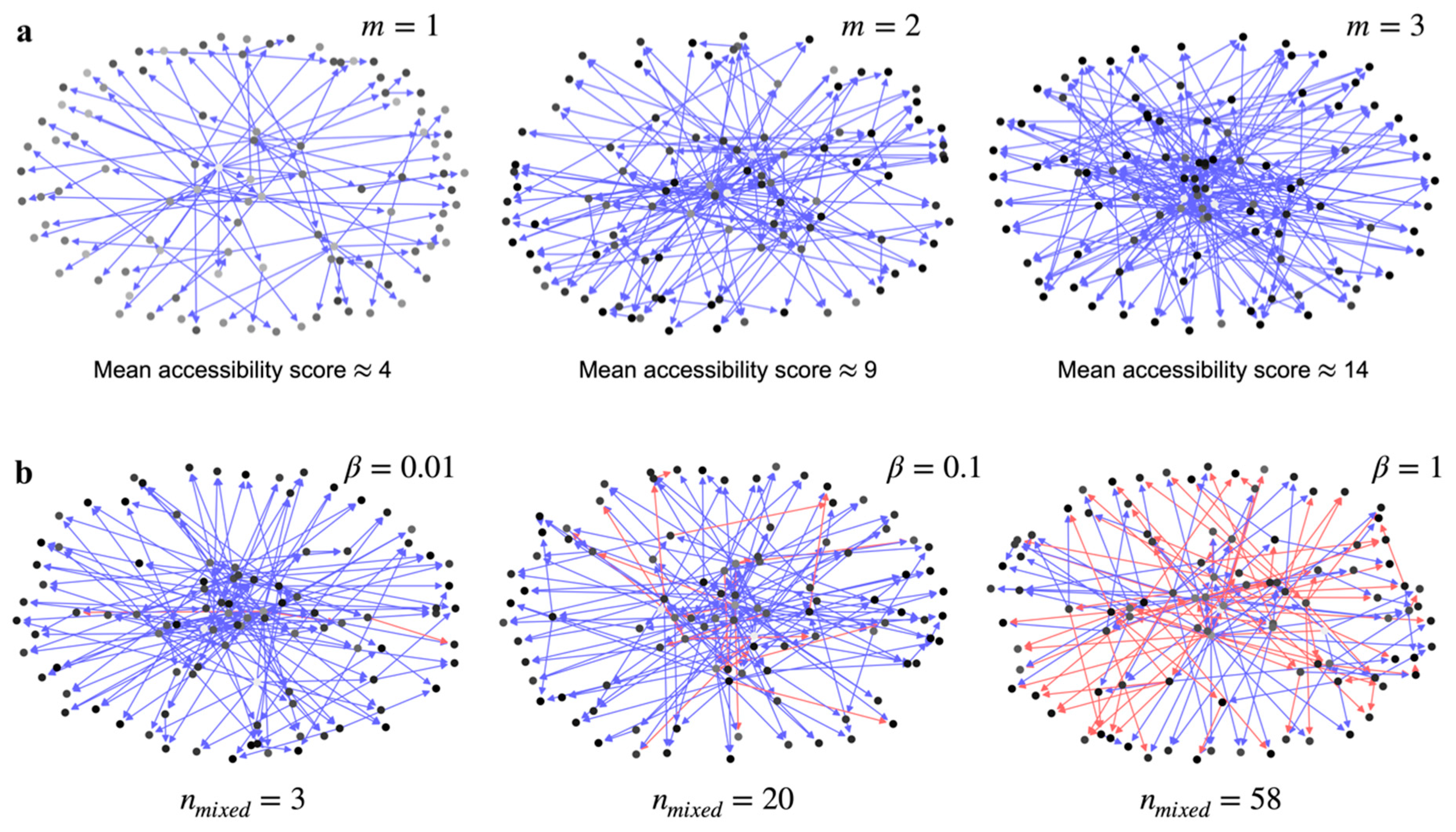
Increasing
increases the number of nodes in the GRN that have a path to a single node, which we refer to as the accessibility score (
Section S3). This is illustrated in
Figure 1a using three Barabási–Albert graphs with
, 2, and 3, respectively. Every node is shaded in proportion to the number of other nodes in the graph that can access it—a node with a darker shade means more nodes have a path to it. Rather than the distribution of shades in a single graph in
Figure 1a, it is more important to note the global prevalence of darker shade nodes with increasing
. The increasing fraction of darker shaded nodes means an increase in global accessibility across all the nodes in the network (
Figure S1). The mean accessibility score, or the average accessibility to a node from all other nodes in the network, increases with
by design.
The other factor that can reduce the effective information transfer is the mixture of up and down regulation signals to a given node in the network.
Figure 1b shows that how increasing the ratio of downregulation edges to the upregulation edges in the graph,
, increases the number of nodes in the graph that are receiving mixed signals,
. If the signal from a source node forks into two separate pathways to a receiver node, and one path ends with an upregulation edge and the other with a downregulation edge, then the effective information transfer to the receiver node is reduced.
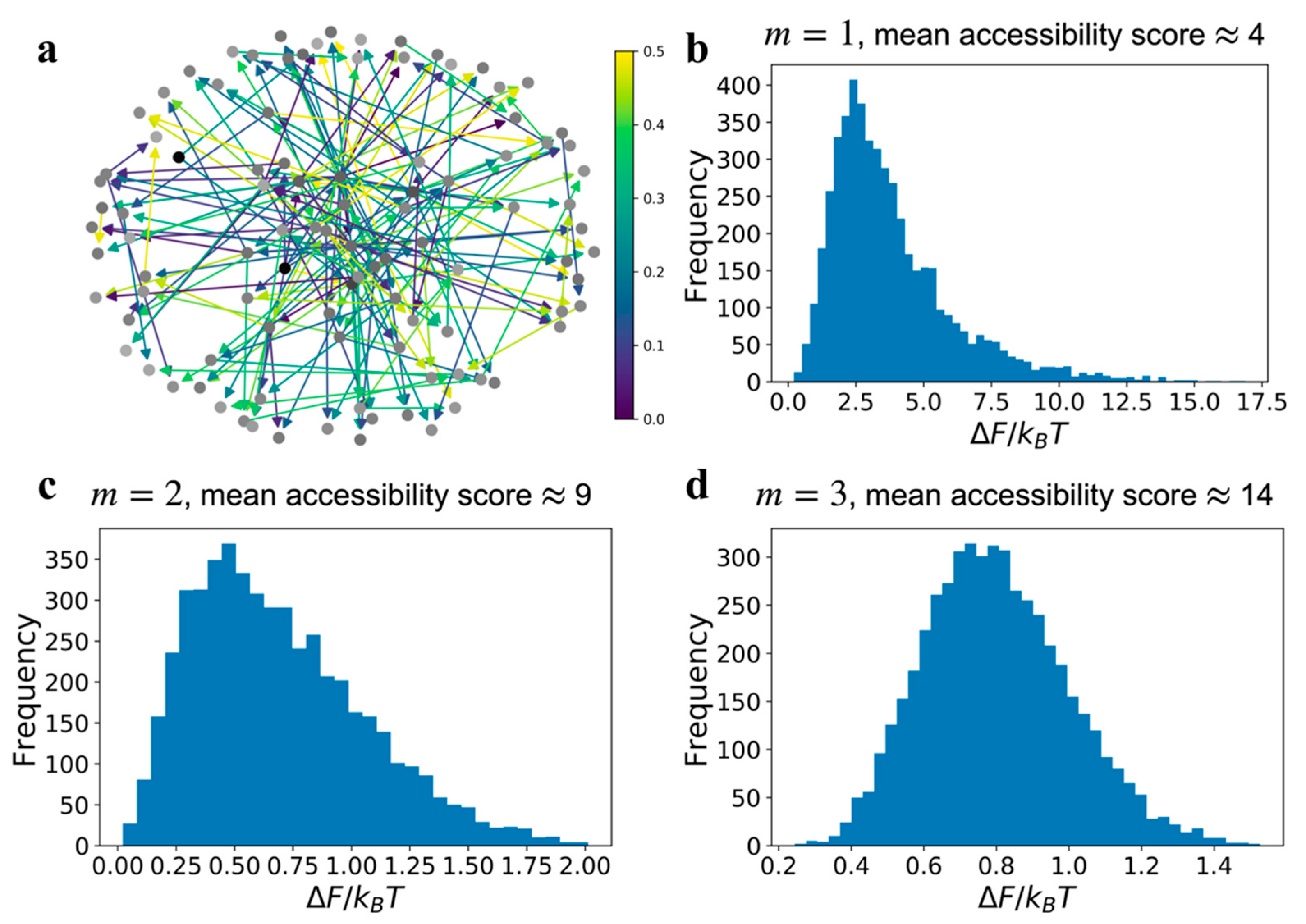
As illustrated in
Figure 2a, the state of a receiver node,
, is determined by the states of all contributing source nodes, using Equations (3) and (4). The 3rd panel of
Figure 2a shows that when all the source nodes are at maximum entropy, the receiver node is also at maximum entropy and independent of up or downregulation and the edge bit-flip error,
. On the other hand, when a single source node,
, is at low entropy, then the bit-flip error values for the edges on the source-receiver path determine the state of the receiver node as shown in the first and second panels of
Figure 2a. Furthermore, the state of the receiver node is superposed with the maximum entropy state of the other source nodes. Therefore, the low entropy input from a single source gains entropy as a function of the edge bit-flip errors and from superposition from other sources. The information loss field computation using Equations (3)–(6) determines the effect demonstrated in
Figure 2a for GRNs involving a large number of genes and complex information propagation pathways.
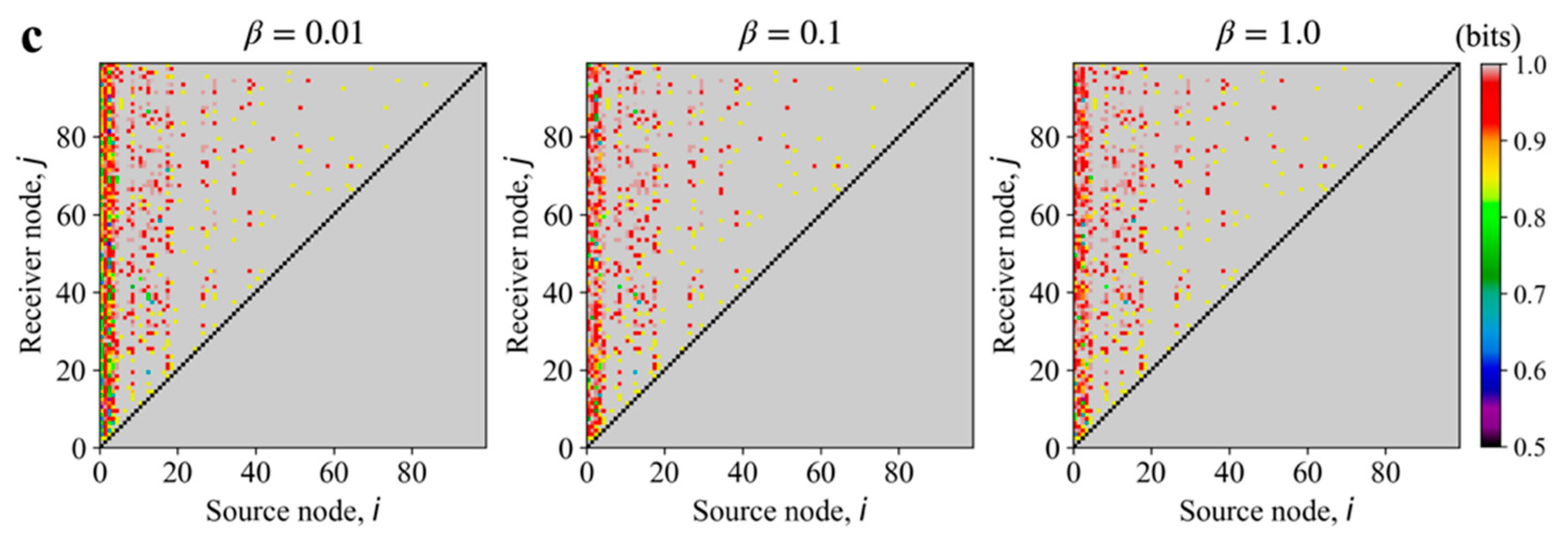
When we evaluate the loss field for every source-receiver pair in the model GRNs shown in
Figure 1a, we notice that the information loss due to superposition increases markedly with increasing
, as shown in
Figure 2b. The sensitivity of the loss field to the in-degree
, also depends on the edge bit-flip error value
. When the bit-flip error is small,
(1st row in
Figure 2b), then the contrast between the loss field for
and
is significant, increasing approximately from 0.2 bits to 0.9 bits. When the bit-flip error is larger,
(2nd row in
Figure 2b), then the increase in loss field from the
type GRN to
is smaller, approximately from 0.8 bits to 1 bit. Hence, the loss field quantifies the effective deterioration of signaling due to combination of superposition and edge communication errors. Though the
type GRN has more source-receiver pairs compared to the
type GRN, abundance of accessibility reduces the quality of communication as apparent in the respective loss fields.
As evident from the loss fields in
Figure 2b, a low entropy input of
or
from a single source node can be diminished if high entropy information from the rest of the source nodes in the graph is superposed on the receiver, leading to a high global entropy for the network. Therefore, for graphs with a high mean accessibility score, which increases with
, it is harder to control or correlate the state of all the nodes in the GRN using a single source node without cooperation from other source nodes. The increase in information loss with increasing
is most prominent for the dominant source nodes, which can send information to all the nodes in the graph (near 0 on the source node axis in
Figure 2b).
Increasing the ratio of up and down regulation edges (
) for a fixed GRN increases the loss field value only for the dominant source nodes as shown in
Figure 2c, which in this example are the first five source nodes (
). Increasing the mixture of up and down regulation does not change the loss field for the lower ranked source nodes, i.e., the source nodes that can propagate information to only a small subset of the receiver nodes in the GRN. Moreover, comparing
Figure 2b,c reveals that information loss is more greatly affected by the increase in superposing pathways (i.e.,
) than by the increasing mixture of up and downregulation.
The large difference in loss field contrasts between
and
in
Figure 2b suggests that we can claim that network of type
allows for an ideal master regulator that can communicate to all the other nodes in the GRN with minimal information loss when the communication error in every single edge is low. The value of loss for the
GRN is high because of the existence of many pathways, so it is challenging for a single node (or gene) to emerge as a master regulator. Therefore, a relatively low number of superposing pathways supports the existence of a master regulator and can be an indicator of a reducible network, unless the communication error in the edges is very high.
4. Relative Free Energy and Reducibility of GRNs
The method of calculating the effective transition matrix, Equation (5), and the loss field, Equation (6), has a direct thermodynamic interpretation. Low information loss between a pair of genes means the network topology and the edge communication error values are such that there exists high mutual information, or correlation, between the states of two genes. Parrondo et al. has shown that the existence of high mutual information between the two components of a system equates to a proportionate increase in the nonequilibrium free energy of the system [
16]. Since the amount information loss, or mutual information, is a consequence of the information propagation in GRNs, Equation (4), we can effectively compute the free energy change associated with the information propagation.
More specifically, a lower information loss, Equation (6), from a source gene
to a receiver gene
means when the source node is at low entropy then the receiver node is also close to a low entropy state. But if the information loss from
to
is high, then the receiver node is closer to the maximum entropy state. A set of low loss values from a single source node to all the other nodes in the network, like for the source node
in the
type GRN for
shown in
Figure 2b, means a single source node shifts all the other nodes in the network close to a low entropy state. The relative entropy of the state of an individual node with respect to the maximum entropy state,
, provides the relative free energy of a single node. Summing over this relative entropy over all the nodes in the network determines the relative free energy induced by the single low entropy source node. Therefore, the reduction in entropy of all the nodes due to information propagation results in an increase in the free energy of the network with respect to the maximum entropy state of the network.
The highest entropy state of a network is the equilibrium state where each node is in the maximum entropy state,
. Changing the state of a single source node, either to
or to
and propagating the information using Equation (4) to achieve the stationary state,
, results in moving individual nodes from the highest entropy state to a lower entropy state. The relative free energy associated with the global lower entropy stationary state
is,
where
is the stationary state of node
when the source node
is ON. We can similarly compute a free energy change due to
or due to any other state of the input,
. Since each edge in the model GRNs is a binary symmetric channel, the free energy change in the network due to setting a node
to
or
is the same.
Therefore, we anticipate that the lower loss field for source node
for the graph
shown in
Figure 2b means that a single source node can push the entire GRN to a lower entropy more successfully than the other two cases (for
or 3). So, for
type graphs the relative free energy of the GRN due to the low entropy state of source node
should be higher than for graphs where
.
In
Figure 3 we present network relative free energy distributions resulting from edge errors, as a function of signal superposition. Unlike the loss field results in
Figure 2b,c, which were for graphs with the same communication error value
, we assumed that the communication error for an edge is a uniformly distributed random variable in the domain [0,0.5]. The distributions in relative free energy for each type of network, i.e.,
m = 1, 2, or 3, were obtained by simulating 5000 replicates of a graph with the same connectivity but a different set of error values for the edges, sampled from the uniform distribution
. An example of type
network with a random edge communication error field is shown in
Figure 3a. This calculation is similar to observing the relative free energy distribution in a cell population, where each cell has the same GRN topology but there exists a variability in edge communication errors within each cell’s network. If the distribution in the edge errors,
, is narrower than a uniform distribution the result will be a reduced variance in the relative free energy distributions shown in
Figure 3.
The relative free energy distribution for
(
Figure 3b) is asymmetric, but for GRNs with high number of superposing pathways, as in
type graphs, the relative free energy is distributed like a normal distribution. The broader distribution suggests that the relative free energy of each replicate network simulation is uncorrelated due to increasing interference. Correlation among replicates is a combined consequence of
and the edge communication error values. If the edge errors are distributed in low range of values, e.g., uniformly distributed between [0.0,0.1] then in spite of the effects of superposition, the probabilistic states (the global state vector
) of the replicates will be closer to each other. However, when the edge errors vary over a wider range, e.g., uniformly distributed between [0.0,0.5], then increasing
, which increases the number of edges and pathways for information transfer, increases the variability in the probabilistic GRN states among replicates. Hence, if a GRN has a high mean accessibility score, then the relative free energy values present in individual cells in a population are more uncorrelated with each other. Since experimentally observed phenotypic manifestations caused by a GRN are a function of the free energy change that are induced by a GRN [
14,
15], we claim the distributions in observed phenotypes are analogous to the distributions in
, especially for the graphs with lower mean accessibility score.
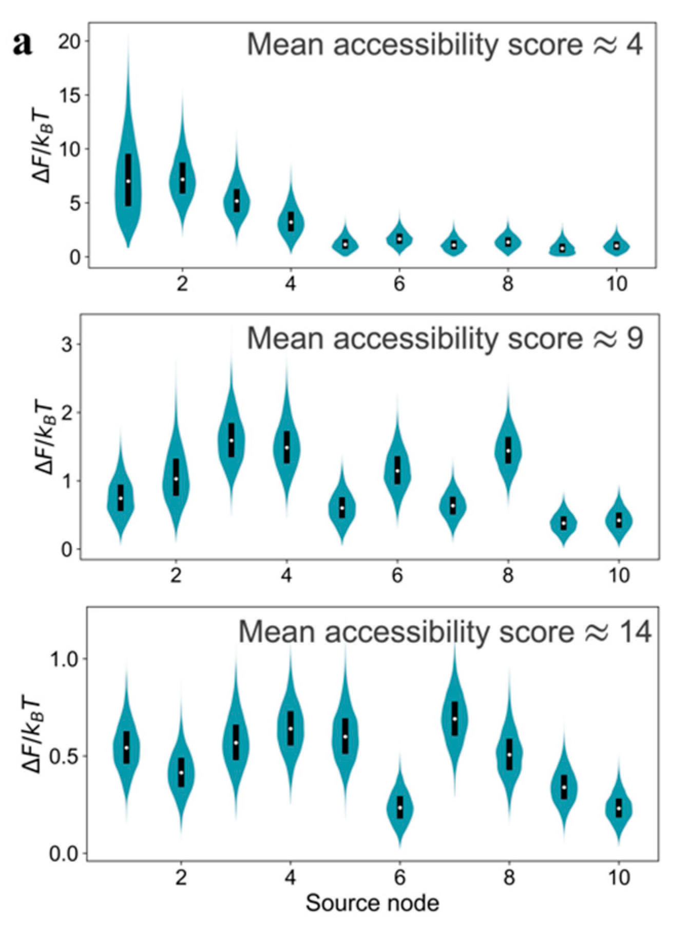
Performing the relative free energy calculations for multiple source nodes in the model GRNs, instead of only the most dominant one, reveals a thermodynamic criterion for reducibility.
Figure 4a shows the relative free energy distributions for the top ten source nodes (ranked by the number of other nodes they can send signal to) in the model GRNs due to a uniformly distributed edge error value. An order exists in the relative free energy distributions as a function of source nodes for
type graph. Not only does the source node
induce significantly higher relative free energy compared to the other source nodes, but also the median value of
for the
graph is higher than the value for
and
graphs. Therefore, the relative free energy distributions are a criterion for thermodynamic hierarchy for source nodes and help to identify candidate master regulators in GRNs. Comparison of the
distributions for multiple source nodes reveals whether that hierarchy exists or not. We claim that the existence of a strongly resolvable hierarchy, i.e., ordered median
values and low overlap in the
distributions for different source nodes, implies that the GRN is thermodynamically reducible. In a network with a small
value, most of the communication to other genes originate from the source node that has the highest out-degree, which creates an outgoing communication hub. Whereas, in a network with a large
value, there are multiple pathways for communication among genes in addition to the ones originating from the outgoing hub. However, the presence of several communication pathways is accompanied with the cost of a lower inducible relative free energy and the lack of hierarchy among the source nodes (
Figure 4a). Interestingly, outgoing hubs have been observed in naturally-occurring GRNs [
30,
31], which may be justified using the thermodynamic hierarchy resulting from the relative free energy distributions.
The existence of the order in
distributions is a function not only of topology and also of the distribution in the edge communication error values. We demonstrate this in
Figure 4b using the
distributions for
type graphs, but with increasing the range of values of
. When the edge error value is uniformly distributed within a more constricted range,
, we still observe a strong hierarchy in
distributions—the median
values for different source nodes are separated beyond the dispersion in the individual distributions. However, this hierarchy is lost upon increasing the extent of variability in
to uniformly distributed in [0.0,0.5], the
distributions for different source nodes become similar to each other, and the median
values decrease for all the source nodes compared to the two narrower distributions in
. Thus, increasing variability in edge error values diminishes the possibility of the existence of a small subset of thermodynamic master regulators.
The choice of a probabilistic edge error field instead of a fixed error value for all edges is a better model for real biological GRNs. For a specific regulatory process, the set of intracellular reactions is the same for all cells in a steady state population. We explicitly considered variability in
, which could result from stochastic fluctuations in concentrations, binding rates, diffusion, etc, due to heterogeneity in the internal environment of the cells. Therefore, the variability in the edge error values result in the distributions of
. In fact, experimental observations of the heterogeneity in gene expression in steady state distributions of cell population phenotypes resulting from [
14] are highly reminiscent of the frequency distributions shown in
Figure 3. We have previously demonstrated that distributions of phenotypes in cell populations represent microstates of a potential landscape, which is consistent with these observations of distributions in
.


