Abstract
Graph enumeration with given constraints is an interesting problem considered to be one of the fundamental problems in graph theory, with many applications in natural sciences and engineering such as bio-informatics and computational chemistry. For any two integers and , we propose a method to count all non-isomorphic trees with n vertices, self-loops, and no multi-edges based on dynamic programming. To achieve this goal, we count the number of non-isomorphic rooted trees with n vertices, self-loops and no multi-edges, in time and space, since every tree can be uniquely viewed as a rooted tree by either regarding its unicentroid as the root, or in the case of bicentroid, by introducing a virtual vertex on the bicentroid and assuming the virtual vertex to be the root. By this result, we get a lower bound and an upper bound on the number of tree-like polymer topologies of chemical compounds with any “cycle rank”.
1. Introduction
Counting and generation of discrete objects are two fundamental problems in combinatorial mathematics and have many applications in the fields of natural science and engineering, such as computational chemistry and bioinformatics. The counting problem asks to count all possible objects under given constraints. On the other hand, the generation problem asks to list all possible objects under given constraints. One of the notable advantages of the counting problem is that we can know the size of the solution space before generating all solutions.
Different kinds of enumeration methods are used to solve counting and generation problems, where branching algorithms and Polya’s enumeration theorem are the two most commonly used methods for these problems. In branching algorithms, the computation is performed by following a computation tree, and the required solutions are attained at the leaves of the computation tree. It is important to mention that the branching algorithms can only count all solutions after generating each one of them, and therefore they are inefficient for the problem where we first want to know the size of the solution space before the generation of solutions.
The well-known Polya’s enumeration theorem [1,2] is used for counting all distinct objects. The idea of this method is to use the cyclic index of the group of symmetries of the underlying object to develop a generating function, which is then used to count all possible objects. Note that finding the group of symmetries and its cyclic index is a challenging task, which may make the use of Polya’s theorem harder for some problems.
The drawback of branching algorithms discussed above and the difficulty of using Polya’s theorem necessitate the exploration of new enumeration methods to solve counting problems efficiently. For an enumeration method, it is necessary to satisfy the following three conditions:
- (i)
- Consider all solutions: The method does not miss any of the required objects;
- (ii)
- Avoid duplication: The method does not count and generate isomorphic objects; and
- (iii)
- Low computational complexity: The method can count and generate all solutions in low time and space complexity.
Designing such a method is not an easy task, because of the underlying symmetries and the computation difficulty for their detection.
Counting and generation of chemical compounds have a long history and numerous applications in designing novel drugs [3,4,5,6,7,8] and structure elucidation [9]. The problem of counting and generation of chemical compounds can be viewed as the problem of enumerating graphs with given constraints. There are several available chemical compound enumeration tools [10,11,12]. We can divide these tools into two classes. One class of enumeration tools treats general graph structures [10,12]. In the other class, the tools are focused on enumerating some restricted chemical compounds. One such tool is Enumol2 [11]. Enumeration of restricted chemical compounds with specialized tools is more efficient than with the tools which use general graph structures. This led to a new trend of developing efficient enumeration of restricted chemical compounds in the field of chemoinformatics [13].
A polymer is a large molecule with interesting chemical properties consisting of many sub-molecules. From a graph-theoretic perspective, we represent the structure of a polymer with a graph G called polymer topology, possibly with self-loops and multi-edges, such that G is connected and the degree of each vertex in G is at least three [14]. For a chemical graph, we get its polymer topology by repeatedly removing the vertices of degree one and two. For example, the polymer topology of Remdesivir CHNOP Figure 1a, a potential candidate of treatment for COVID-19, is illustrated in Figure 1b.
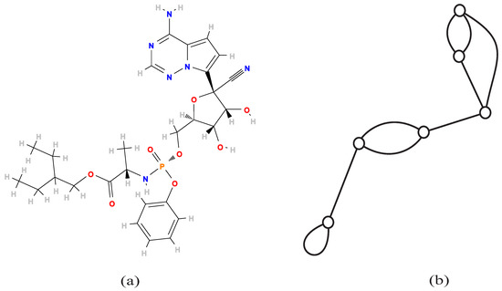
Figure 1.
The chemical compound Remdesivir CHNOP and its polymer topology: (a) chemical structure of Remdesivir CHNOP obtained from the PubChem database; (b) the polymer topology of Remdesivir with six vertices, two multi-edges of multiplicity 2, one self-loop and cycle rank 4.
Tezuka and Oike [15] pointed out that a classification of polymer topologies will lay a foundation for the elucidation of structural relationships between different macro-chemical molecules and their synthetic pathways. Different kinds of graph-theoretic approaches have been applied to classify and enumerate polymer topologies [16,17]. For a connected graph G, possibly with self-loops and multi-edges, the cycle rank is defined to be the number of edges that must be removed to get a simple spanning tree of G. Recently, Haruna et al. [14] proposed a method to enumerate all polymer topologies with cycle rank up to five.
Notice that trees with no multi-edges but with self-loops have cycle rank and include all polymer topologies with the said structure. Therefore, it is of interest to count and generate all trees with no multi-edges and a given number of vertices and self-loops.
We use dynamic programming (DP) to count all mutually non-isomorphic trees with n vertices, self-loops and no multi-edges. The basic idea of DP is to partition the original problem into subproblems that satisfy some recursive relations, and the union of their solution sets is equal to the solution set of the original problem. Unlike branching algorithms and Polya’s theorem, the main advantage of using the DP is that we can count all non-isomorphic structures without their generation and calculation of their group of symmetries. As an application of our results, we get lower and upper bounds on the number of tree-like polymer topologies with self-loops of a given cycle rank.
2. Preliminaries
Throughout this draft, the term graph stands for an undirected graph with no multi-edges and possibly with self-loops unless stated otherwise. Let G be a graph. We denote an edge between two vertices u and v in G by . Let and denote the vertex set and edge set of G, respectively. Let denote the number of self-loops in G. For a vertex , we denote by the number of self-loops on the vertex v. For a vertex v in G, let denote the set of vertices incident to v except v itself and the degree deg of v in G is defined to be . A graph H with the properties and is called a subgraph of G. A simple path between two distinct vertices is defined to be a subgraph P of G with vertex set and edge set . A graph is called a connected graph if there is a path between any two distinct vertices in the graph. A connected component of a graph G is defined to be a maximal connected subgraph H of G, i.e., for any vertex it holds that every subgraph with the vertex set is disconnected.
By Jordan [18], any simple tree with vertices has either a unique vertex or edge, the removal of which creates connected components with at most or exactly vertices, respectively. Such a vertex is called the unicentroid, the edge is called the bicentroid, and collectively they are called the centroid of the tree. It is important to note that there exits a bicentroid only for trees with an even number of vertices. A tree with a fixed vertex r is called a rooted tree with root r. Note that any tree can be uniquely viewed as a rooted tree by either regarding its unicentroid as the root, or in the case of a bicentroid, by introducing a virtual vertex on the bicentroid and assuming the virtual vertex as the root.
Let H be a rooted tree. Let denote the root of H. For any two distinct vertices , let denote the unique simple path between them in H. For a vertex , we define the ancestors of v to be the vertices on the path other than v. If u is an ancestor of v, then we call v a descendant of u. For a vertex , the parent of v is defined to be the ancestor u of v such that . We call the vertex v a child of . Two vertices with the same parent in H are called siblings. For a vertex , let denote the subtree of H rooted at v induced by v and its descendants.
Two rooted trees T and H are called isomorphic if there exists a bijection such that
- (i)
- ;
- (ii)
- for each vertex , it holds that ; and
- (iii)
- for any two vertices , it holds that if and only if .
For any two integers and , let denote a maximal set of mutually non-isomorphic rooted trees with n vertices and self-loops, and we define .
3. Counting Tree-Like Graphs with a Given Number of Vertices and Self-Loops
We develop a method to compute for any two integers and , the size of a maximal set of mutually non-isomorphic rooted trees with n vertices and self-loops; i.e., we are interested in the following problem:
Counting Problem
Input: Two integers and .
Output:
We solve this problem by using dynamic programming based on the information of the number of vertices and self-loops in the subtrees rooted at the children of the root of each tree in . We define the following notions.
Let and be any two integers. For each tree , we define
Note that for any tree , it holds that and .
Let be any two integers. We define
Observe that by the definition of it holds that
- (i)
- if ;
- (ii)
- if ; and
- (iii)
- .
Therefore, from now on, we assume that and . Further, by the definition of it holds that (resp., ) if “” or “” (resp., otherwise ( and )).
We define
It follows from the definition of that (resp., ) if “” or “” (resp., otherwise ( and )). Further we have the following relation:
where for .
Next we define
Note that if “ and ” or “” (resp., otherwise (“ and ” or “ and ”)), then by the definition of it holds that (resp., ). Furthermore, we get the following relation for :
where for .
Let , and be four integers. Let , and denote the number of elements in the families , and , respectively. We discuss recursive relations for and in Lemma 1.
Lemma 1.
For any four integers , and , it holds that
- (i)
- if ;
- (ii)
- if ;
- (iii)
- if ; and
- (iv)
- if .
Proof.
Next we discuss some boundary conditions for our DP to compute
Lemma 2.
For any four integers , and , it holds that
- (i)
- (resp., ) if and (resp., otherwise (“ and ” or “ ”));
- (ii)
- (resp., ) if (resp., otherwise ());
- (iii)
- if “ ” or “ and ”; and
- (iv)
- if “ ” or “ and ”.
Proof.
- (i)
- The result follows from the definition of , since a tree H with max exists if and only if and max.
- (ii)
- By Lemma 1(i), (ii) and (iv) it holds that . This and Lemma 2(i) imply the required result.
- (iii)
- When , then for any tree it holds that . Thus for each it holds that and if “” or “ and ”, i.e., . But by Lemma 2(ii) it holds that . Hence we have the required result.
- (iv)
- Let “” or “ and ”. By Lemma 1(iii) and (iv) it holds that . This and Lemma 2(iii) imply thatFurthermore, by Lemma 1(iii) it holds that . By Lemma 2(ii), we have . Hence the result follows by Equation (5).
□
By Lemma 2, we can get that and . Furthermore, Lemma 1(i)–(iv) give recursive relations for and which depend on . Thus for , , and , our next goal is to develop a recursive relation for . For any tree and any vertex , the subtree of H satisfies exactly one of the following three conditions:
- (C-1)
- and
- (C-2)
- and
- (C-3)
- and
For any tree , we define the residual tree of H to be the subtree of H rooted at induced by the vertices Note that the residual tree of a tree H has at least one vertex, i.e., the root of H. We give an illustration of a residual tree in Figure 2.
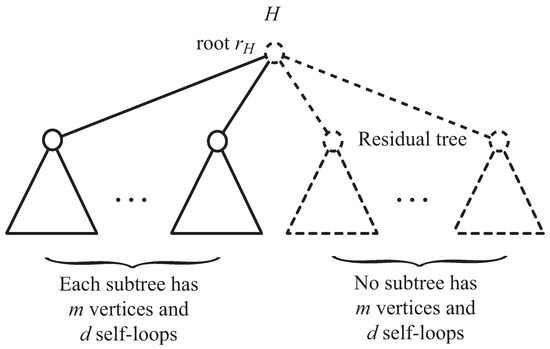
Figure 2.
An illustration of a residual tree, where and the residual tree of H is shown by dashed lines.
Lemma 3.
For any four integers , , and , and a tree let . Then it holds that
- (i)
- with when .
- (ii)
- The residual tree of H belongs to exactly one of the families and .
Proof.
- (i)
- Since , there exists at least one vertex such that . This implies that . Also, it holds that and . This implies that with when .
- (ii)
- Let K denote the residual tree of H. By the definition of K it holds that . Furthermore, for each vertex the tree satisfies exactly one of the conditions (C-2) and (C-3). Now, if there exists a vertex such that satisfies condition (C-2), then , and hence . On the other hand, if condition (C-2) does not hold for any ; i.e., either or for each it holds that and , then by the definition of K it holds that This completes the proof.
□
For any five integers , , , and , let denote the number of combinations with repetition of t trees from the family . In Lemma 4, we give a recursive relation for .
Lemma 4.
For any five integers , , , and q, such that with when , it holds that
- (i)
- if ;
- (ii)
- if ;
- (iii)
- if ; and
- (iv)
- if .
Proof.
Let H be a tree in the family . By Lemma 3(i), there exists a unique integer q, with when , such that there are exactly q subtrees with and . Further, by Lemma 3(ii) the residual tree of H belongs to the family (resp., if (resp., otherwise). Note that . This implies that for a fixed integer q in the range given in the lemma, the number of trees K in the family with exactly q subtrees , for , are
- (a)
- if ; and
- (b)
- if .
Note that, for and , we have , and by Lemma 2(ii) it holds that (resp., ), if (resp., otherwise (if )). This implies that any tree has exactly subtrees , for . However, observe that for each integer or , and q satisfying the conditions given in the lemma, there exists at least one tree such that H has exactly q subtrees , for . Hence, this and case (a) (resp., case (b)) imply Lemma 4(i) (resp., Lemma 4(ii)).
Furthermore, it holds that
Hence, Lemma 4(iii) and (iv) follow from Lemma 4(i) and (ii), respectively. □
We design a DP algorithm to compute based on the recursive structures of , and , and , as given in Lemmas 1 and 4, where for and .
Lemma 5.
For any four integers , and , can be obtained in time and space.
The proof of Lemma 5 follows from Algorithm 1 and Lemma 6.
Corollary 1.
For any two integers and can be obtained in time and space.
Next, for any four integers , and , we present Algorithm 1 for solving the problem of calculating . In this algorithm, for each integers , and , the variables , , and store the values of and , respectively.
Lemma 6.
For any four integers , and , Algorithm 1 outputs in time and space.
Proof.
Correctness: For each integer , and , all the substitutions and if-conditions in Algorithm 1 follow from Lemmas 1, 2, 3 and 4. Furthermore, the values , , and are computed by the recursive relations given in Lemmas 1 and 4. This implies that Algorithm 1 correctly computes the required value .
Complexity analysis: There are three nested loops over the variables and p at line 4, which take time. Following there are five nested loops: over variables , and q at lines 5, 6, 7, 8, and 31, respectively. The loop at line 5 is of size , while the loop at line 6 is of size . Similarly, the loops at lines 7 and 8 are of size and , respectively. The fifth nested loop at line 18 is of size (resp., ) if (resp., otherwise). Thus from line 5–36, Algorithm 1 takes (resp., ) time if (resp., otherwise). Therefore, Algorithm 1 takes time.
The algorithm stores three four-dimensional arrays. When , for each integer , and we store and , taking space. When , then for each integer , , and we store and , taking space. Hence, Algorithm 1 takes space. □
| Algorithm 1 DP based counting algorithm for |
| Input: Integers and . |
| Output:. |
| ; |
| ; |
| for each , ; |
| for do |
| for do |
| for do |
| for do |
| if and then |
| else /* or */ |
| ; /* Initialization */ |
| if then |
| else /* */ |
| end if; |
| for do |
| if then |
| else /* */ |
| end if |
| end for; |
| if then /* */ |
| else /* */ |
| end if; |
| end if |
| end for |
| end for |
| end for |
| end for; |
| output as . |
Theorem 1.
For any two integers and , the number of non-isomorphic trees with n vertices and Δ self-loops can be obtained in time and space.
Proof.
By Jordan [18], we can uniquely consider any tree as a rooted tree by either regarding its unicentroid as the root, or in the case of a bicentroid, by introducing a virtual vertex on the bicentroid and assuming the virtual vertex as the root of the tree. By the definition of a unicentroid, the number of mutually non-isomorphic trees with n vertices, self-loops and a unicentroid is . Further, if n is even, then there exist trees with n vertices and a bicentroid. This implies that the number of mutually non-isomorphic trees with n vertices and self-loops is when n is odd. Let n be an even integer. Then any tree H with n vertices, self-loops and a bicentroid has two connected components, A and B obtained by the removal of the bicentroid such that and for some , where if is even then for , both of the components A and B belong to .
Note that for any , it holds that
Therefore, when is odd (resp., even), the number of mutually non-isomorphic trees with n vertices, self-loops, and a bicentroid is
such that (resp., ). Thus, the number of mutually non-isomorphic trees with n vertices and self-loops is
such that (resp., ) when is odd (resp., even). Moreover, for each , Algorithm 1 also computes and stores during the calculation of , and therefore the required result follows from Lemma 6. □
We implemented the proposed DP algorithm and counting trees with a given number of vertices and self-loops. The experimental results in Table 1 show that the proposed method efficiently counts trees with n vertices and self-loops.

Table 1.
Experimental result of the counting method.
We next give a lower bound and an upper bound on the number of tree-like polymer topologies with self-loops of a given rank. For this we prove the following results.
Lemma 7.
For an integer , there exists at least one tree-like polymer with n vertices and Δ self-loops if .
Proof.
Consider a tree T of n vertices of diameter such that T contains a path of length , in which each non-end vertex has degree at least 3. Observe that when n is even, the tree T has exactly vertices of degree 3, and hence vertices of degree less than 3. When n is odd, the tree T has vertices of degree 3 and one vertex of degree 4. Thus, in this case, the number of vertices of degree less than 3 is This implies that T can be transformed into a polymer with self-loops by assigning a self-loop to each vertex of degree less than 3. Hence, self-loops are sufficient to get a tree-like polymer with n vertices. □
For two integers and , let denote the number of trees with n vertices and self-loops. For , let denote the number of tree-like polymers with self-loops and no multi-edges of rank r. Observe that a tree with n vertices and k self-loops at each vertex is a polymer with n vertices of cycle rank . From this fact and Lemma 7 it holds that
4. Conclusions
This paper presented an efficient method to count the number of all mutually non-isomorphic trees with a given number of vertices and self-loops. The proposed method is based on dynamic programming where we count the number of all mutually non-isomorphic rooted trees with a given number n of vertices and self-loops in time and space. As an application of our results, we gave lower and upper bounds on the number of tree-like polymer topologies with a given cycle rank. This is an interesting application of DP to objects such as trees, and offers the advantage of getting the size of the entire solution space at low computational complexity without explicitly generating each object.
An interesting direction for future research is to efficiently generate all mutually non-isomorphic trees with a given number of vertices and self-loops by using the result from the developed counting method. Further, another possible extension of this research is to count and generate all mutually non-isomorphic tree-like polymer topologies with a given number of vertices and self-loops.
Author Contributions
Conceptualization, N.A.A. and H.N.; funding acquisition, N.A.A.; methodology, N.A.A. and H.N.; software, N.A.A.; supervision, H.N.; validation, N.A.A., A.S. and H.N.; writing—original draft, N.A.A.; writing—review and editing, N.A.A. and A.S. All authors have read and agreed to the published version of the manuscript.
Funding
This research is partially funded by JSPS KAKENHI Grant Number 18J23484.
Conflicts of Interest
The authors declare no conflict of interest.
References
- Pólya, G. Kombinatorische anzahlbestimmungen für gruppen, graphen und chemische verbindungen. Acta Math. 1937, 68, 145–254. [Google Scholar] [CrossRef]
- Polya, G.; Read, R.C. Combinatorial Enumeration of Groups, Graphs, and Chemical Compounds; Springer Science & Business Media: New York, NY, USA, 2012. [Google Scholar]
- Blum, L.C.; Reymond, J.L. 970 million druglike small molecules for virtual screening in the chemical universe database GDB-13. J. Am. Chem. Soc. 2009, 131, 8732–8733. [Google Scholar] [CrossRef] [PubMed]
- Azam, N.A.; Chiewvanichakorn, R.; Zhang, F.; Shurbevski, A.; Nagamochi, H.; Akutsu, T. A method for the inverse QSAR/QSPR based on artificial neural networks and mixed integer linear programming. In Proceedings of the 13th International Joint Conference on Biomedical Engineering Systems and Technologies—Volume 3: Bioinformatics, Valletta, Malta, 24–26 February 2020. [Google Scholar]
- Ito, R.; Azam, N.A.; Wang, C.; Shurbevski, A.; Nagamochi, H.; Akutsu, T. A novel method for the inverse QSAR/QSPR to monocyclic chemical compounds based on artificial neural networks and integer programming. In Advances in Computer Vision and Computational Biology; Springer Nature-Research Book Series; Springer: Berlin/Heidelberg, Germany, 2020. [Google Scholar]
- Zhu, J.; Wang, C.; Shurbevski, A.; Nagamochi, H.; Akutsu, T. A novel method for inference of chemical compounds of cycle index two with desired properties based on artificial neural networks and integer programming. Algorithms 2020, 13, 124. [Google Scholar] [CrossRef]
- Méndez-Lucio, O.; Baillif, B.; Clevert, D.A.; Rouquié, D.; Wichard, J. De novo generation of hit-like molecules from gene expression signatures using artificial intelligence. Nat. Commun. 2020, 11, 10. [Google Scholar] [CrossRef] [PubMed]
- Lim, J.; Hwang, S.Y.; Moon, S.; Kim, S.; Kim, W.Y. Scaffold-based molecular design with a graph generative model. Chem. Sci. 2020, 11, 1153–1164. [Google Scholar] [CrossRef]
- Meringer, M.; Schymanski, E.L. Small molecule identification with MOLGEN and mass spectrometry. Metabolites 2013, 3, 440–462. [Google Scholar] [CrossRef] [PubMed]
- Benecke, C.; Grund, R.; Hohberger, R.; Kerber, A.; Laue, R.; Wieland, T. MOLGEN+, a generator of connectivity isomers and stereoisomers for molecular structure elucidation. Anal. Chim. Acta 1995, 314, 141–147. [Google Scholar] [CrossRef]
- Available online: http://sunflower.kuicr.kyoto-u.ac.jp/tools/enumol2/ (accessed on 4 July 2020).
- Peironcely, J.E.; Rojas-Chertó, M.; Fichera, D.; Reijmers, T.; Coulier, L.; Faulon, J.L.; Hankemeier, T. OMG: Open molecule generator. J. Cheminf. 2012, 4, 21. [Google Scholar] [CrossRef] [PubMed]
- Vogt, M.; Bajorath, J. Chemoinformatics: A view of the field and current trends in method development. Bioorg. Med. Chem. 2012, 20, 5317–5323. [Google Scholar] [CrossRef] [PubMed]
- Haruna, T.; Horiyama, T.; Shimokawa, K. On the enumeration of polymer topologies. IPSJ SIG Tech. Rep. 2017, 2017-Al-162, 1–5. [Google Scholar]
- Tezuka, Y.; Oike, H. Topological polymer chemistry. Prog. Polym. Sci. 2002, 27, 1069–1122. [Google Scholar] [CrossRef]
- Galina, H.; Sysło, M.M. Some applications of graph theory to the study of polymer configuration. Discret. Appl. Math. 1988, 19, 167–176. [Google Scholar] [CrossRef]
- Zimm, B.H.; Stockmayer, W.H. The dimensions of chain molecules containing branches and rings. J. Chem. Phys. 1949, 17, 1301–1314. [Google Scholar] [CrossRef]
- Jordan, C. Sur les assemblages de lignes. J. Reine Angew. Math. 1869, 70, 81. [Google Scholar]
© 2020 by the authors. Licensee MDPI, Basel, Switzerland. This article is an open access article distributed under the terms and conditions of the Creative Commons Attribution (CC BY) license (http://creativecommons.org/licenses/by/4.0/).