Averaged Optimization and Finite-Time Thermodynamics


Abstract
:1. Introduction
- 1.
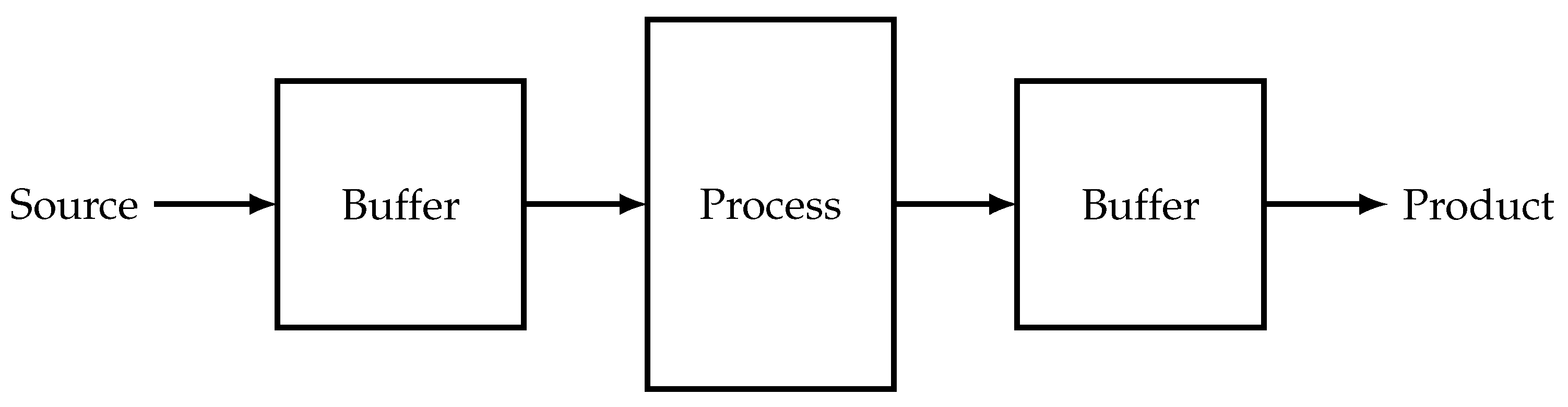
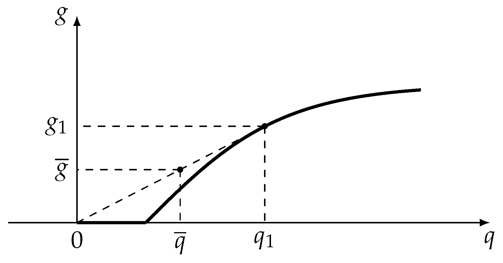
- Assume that there is a bound on the source flow and this constraint lowers the possible optimal value of the production. If we introduce some buffer (container) in such a way that the source flow is its feed, we can raise the possible value of the feed flow to the actual process without violating this constraint. Actual values of the feed flow will oscillate between values that are greater than and less than . Only the mean value of the feed flow will be bounded in this case. Using this approach we can replace the strict constraint on by the averaged one. If we use such a buffer to store the product flow, we can maximize not this flow itself, but its mean value (Figure 1).Let us assume that the relationship between production rate g and consumption q has the form presented at Figure 2.With the help of buffers this relationship could be improved on interval from 0 to . The process must operate with consumption during some fraction of time and with zero consumption during the remaining time. Relationship between average production and average consumption is represented by dashed slope line at Figure 2. This is the way pumps of water towers operate.
- 2.
- Controls often can have only discrete values. For example, the light switch can be either on or off. None of these discrete values satisfy the constraints of the original problem. If there are devices that smooth out any oscillations of control variables, the optimal mode can correspond to the switching strategy that maintains given average values of flows. This kind of switching is the basis of electronic light dampers.
- 3.
- In a heat engine the working fluid periodically makes contacts with the hot and cold sources, and the properties of these contacts must be chosen such that the average properties of the working fluid satisfy the constraints of the optimum cycle problem.
- 1.
- Many processes are periodic and their constraints must be satisfied on average per cycle.
- 2.
- Interactions of thermodynamic systems are characterized by values of extensive variables X (volume, amount of substance, internal energy, entropy), and flows of mass and energy emerging in these interactions depend on intensive variables y (temperature, pressure, molar fraction). The rate of change of extensive variables depend on a flow, and of course on y. This means that the governing equations for thermodynamic interactions have the form:The right hand side of (1) does not contain X and this means that the increase in extensive variables during some given amount of time depends only on the mean value of F. It does not depend on the order in which intensive variables have different values, if the mean value of F remains constant. Equations such as (1) are called Lyapunov-type. They allow us to formulate the problem of optimal control for thermodynamic systems in averaged form.
- The human organism in a steady mode in the absence of external perturbations is characterized by a constant temperature, a constant composition of arterial blood, etc. However, some factors such as the blood pressure and the lung volume periodically change. This is related to the ”structure“ of the respiration and circulation organs.
- A system consisting of a pump connected with a tank (e.g., a water tower) and consumers operates so that, even if the liquid consumption is constant, the pump is sometimes completely switched off (and the liquid does not flow into the tank) and is sometimes switched on and operates with delivery higher than , with the average delivery being . If the dependence of the pump delivery g on the power expenditure S is described by a strictly convex function, then the average pump delivery is higher than that in the static mode at the same average power expenditure.In the rest of the paper, we mainly consider cyclic steady-state modes, among which two limit classes are distinguished. The first class includes modes in which each of the periods significantly exceeds the time of relaxation processes in the system. Moreover, each of the static steady states is assumed to be stable. In this case, we can neglect the dynamics of the system and assume that under variation of the mode variables, the state variables change in accordance with the static characteristics. Such modes are said to be quasi-static.The second class is formed by sliding steady-state modes, in which all or some of the control variables vary with frequency so high that, due to the inertia of the object, the state variables remain virtually constant, and their values depend only on the averaged influence of the control variables.Although static modes are a special case of cyclic modes, below by cyclic modes we mean modes under which at least one variable of the process changes periodically in time. A cyclic mode is said to be efficient if the passage to this mode improves the efficiency of the process in comparison with the static mode.
- Cyclic modes are typical of systems with no admissible static modes. Often a system has no static modes if the set V of admissible values of variables is non-convex; e.g., this set may include only discrete values. This is so, for example, in a heat engine in which a working fluid contacts a heat source whose temperature can take only two values, (a hot source) and (a cold source), and the average power over a cycle is required to be maximal under certain constraints.
- Does there exist a cyclic mode satisfying the constraints of the problem?
- Is the transition from the optimal static mode to the cyclic mode efficient?
- What is the gain in the optimality criterion from this passage?
- What are the optimal forms of variation of the control and state variables, optimality conditions, computational algorithms?
2. Averaged Optimization Problems and Their Optimality Conditions
2.1. Averaging of Functions Included in the Formulation of an Optimization Problem
2.2. Convex Hulls—Carathéodory’s Theorem
- 1
- The convex hull of a set V is the minimum convex set such that .
- 2
- The set of points lying on or below the graph of a function is called its hypograph. The convex hull of a function f is the upper boundary of the convex hull of its hypograph.
- 3
- Alternatively, the convex hull of a function f is the minimum convex function defined on the convex hull of the domain of f. For every from the domain of f the following holds: .
2.3. Optimal Distribution in An Averaged NLP Problem
2.4. Necessary Conditions of Optimality—Kuhn-Tucker Theorem
2.5. Reduction to an Ordinary NLP Problem
2.6. Relationship between Averaged NLP Problem and the Lagrangian Function of the NLP Problem without Averaging
2.7. Other Forms of Averaged Extensions of the NLP Problem
- Problem of maximizing a function of the mean value of the argument. When D is the set of admissible solutions of the initial NLP problem, i.e., D is defined by the condition , and is the mean value of the vector x on the set D, we have:Since the set of values satisfying this condition is the convex hull of D, problem (24) is equivalent to the NLP problem on the convex hull of D:
- Problem of maximizing the mean value of a function under constraints imposed on the mean value of the argument:or, in more detail,
- Problem of maximizing a function of the mean value of x under averaged constraints:
2.8. The Algorithm for Obtaining Optimality Conditions in Averaged Problems
- Is the optimal distribution, which is one of the components of the solution of an averaged problem, always concentrated at finitely many base points?
- If the answer to the previous question is ”yes,“ then what is the limit number of these points?
- separates the randomized and deterministic variables;
- calculates the total number L of averagings, which is equal to the sum of the dimensions of the vector of randomized variables and of the vector of functions to be averaged;
3. Non-Stationary Problems of Averaged Optimization
- on the interval of variation of the parameter
- on the total constancy interval of , the optimal solution switches between at most base values , and each of these values satisfies the condition
- the portions of the constancy interval on which takes the respective values satisfy the conditions
- the vector of multipliers , , is determined by the conditions
4. Estimation of the Performance of Cyclic Modes
5. Estimation of the Efficiency of Transition to a Cyclic Process
5.1. Conditions of Equivalence and Efficiency of a Cyclic Extension
- An upper bound for and sufficient conditions for the equivalence of a cyclic extension. Let us enlarge the set of admissible solutions of Problem C by removing the differential equations (63). We obtain Problem , which we call an estimating problem:Clearly,and Problem is an averaged extension of Problem S with the variables x and u and the parameters a. The roles of the variables x and u in the conditions of Problem are similar, and we unite these variables and denote them by . In shorthand notation, this problem has the formThe value of problem (78) as an extension of the optimal static mode problem can be expressed in terms of the function asFor determining the vector of parameters, we have the conditionIf lies inside , then condition (80) reduces to the condition of stationarity of with respect to a.If the value given by (79) equals (i.e., Problem has a unique base solution), then inequalities (74) and (77) imply i.e., the static mode cannot be improved by passing to a cyclic mode. If , then the difference between these values gives an upper bound for the possible gain from the passage to a cyclic mode.
- A lower bound for Quasi-static and sliding modes. Consider the case when and vary so that the time derivatives of can be neglected. Then the relations between x and u are given, as in the static case, by for all The corresponding modes are said to be quasi-static. The problem of an optimal choice of and under the quasi-static conditions (Problem QS) has the formor, in shorthand notation,Here and the set is determined by the conditions and .Since any solution of Problem QS is admissible for Problem C, it follows thatAt the same time, the value of Problem QS, being the value of an averaged problem, is given by the expressionHere is the optimal value of a subject to the constraintin which is the set of variations allowed by the inclusion .We choose the Lagrange multipliers in (84) so that for any base value of the vector y. The number of base values of y is determined by the dimension r of the vector function ; thus, the problem takes the formConsider the case when the control vector in the steady state of the system changes with a frequency so high that the state vector x remains virtually constant. Such a mode is called a sliding steady mode. The optimization problem for such a mode is formulated asThis problem is known as Problem SL. In (86), b denotes the vector formed by x and a. This mode is the limit case of the cyclic mode, so we haveProblem (86) is an averaged extension of Problem S with two types of variables; its value is given bywhere satisfies the conditionThe number of base values of the vector function u in Problem SL is at most .A necessary condition for the efficiency of the transition to a cyclic mode can be stated in terms of and . Consider the quantityIf is greater than , then the passage to a cyclic mode is efficient, and the differenceprovides a lower bound for the efficiency.
5.2. The Frequency Criterion for the Efficiency of the Passage to a Cyclic Mode
5.3. Lyapunov Problems
6. Average Optimization in Finite-Time Thermodynamics
- Problems of optimal thermodynamic cycles.There are a very important kind of thermodynamic systems — intermediary ones. These systems contact different subsystems (reservoirs) alternately while producing power and thus lowering the irreversibility arising from a continuous contact of the above-mentioned subsystems. The main example here is the heat engine, where the working fluid contacts two sources of different temperature.One of the most essential problems in finite-time thermodynamics is the problem of maximum average power of heat engines, when the average rate of the heat flow from the hot source is given.Similar problems arise also in absorption-desorption systems, where the working fluid contacts with the multi-component mixture and picks one component out from one source, releasing it at another one.In reverse cycles, the working fluid obtains the energy from the exterior system. Upon contact with the source that loses energy or matter in the regular cycle, the working fluid enriches it with the corresponding resource.In all of these problems, the working fluid restores its state at the beginning of every cycle. One needs to average all of the variables determining the process.
- Relations between intensive and extensive variables are Lyapunov-type equations. Thermodynamic variables are divided into two classes: intensive (temperature, pressure, chemical potential, …) and extensive (volume, internal energy, entropy, amount of substance, …) ones. Flow rates of transport processes between subsystems depend only on intensive variables. This value determines in turn the rate of change of extensive variables. This means that equations determining the change of state of the thermodynamic system have the form [10,11,12]:Here i and j are indices of the contacting subsystems, u is the vector of intensive variables, Z is the vector of extensive variables. Equations of this type are called Lyapunov-type equations earlier in this paper. The right hand side of these equations does not depend on Z, and the increase of Z is determined by the average value of the function F. As we have shown above, one can obtain the limiting capabilities of systems characterized by Lyapunov-type equations using techniques of the averaged optimization.
7. Example: Averaged Optimization of a Heat Engine
7.1. Maximum Average Power Output
7.2. Maximum Efficiency
8. Results
Author Contributions
Funding
Conflicts of Interest
References
- Tsirlin, A.M. Problems and methods of averaged optimization. Proc. Steklov Inst. Math. 2008, 261, 270–286. [Google Scholar] [CrossRef]
- Kaplinski, A.M.; Propoi, A.I. Stochastic Approach to Nonlinear Programming Problems. Automat. Remote Control 1970, 31, 448–459. [Google Scholar]
- Ioffe, A.; Tikhomirov, V. Theory of Extremal Problems; Elsevier North-Holland: New York, NY, USA, 1979; p. 459. [Google Scholar]
- Rockafellar, R.T. Convex Analysis; Princeton University Press: Princeton, NJ, USA, 1996; p. 472. [Google Scholar]
- Boltyanski, V.G.; Martini, H.; Soltan, V. Geometric Methods and Optimization Problems; Springer: New York, NY, USA, 1999; p. 432. [Google Scholar]
- Tsirlin, A. Averaged Optimization Methods and Their Applications (Metody usrednjonnoj optimizatsii i ikh prilozhenija); Fizmatlit: Moscow, Russia, 1997. (In Russian) [Google Scholar]
- Tsirlin, A. Optimal Cycles and Cyclic Modes (Optimal’nye tsikly i tsiklicheskie rezhimy); Energoatomizdat: Moscow, Russia, 1985. (In Russian) [Google Scholar]
- Tsirlin, A.M. Conditions for Optimality of Solutions to Average Problems in Mathematical Programming. Sov. Phys. Dokl. 1992, 37, 117–119. [Google Scholar]
- Tsirlin, A.M. The Optimal Conditions for Averaged Problems with Time-Dependent Parameters. Dokl. Math. 2000, 62, 297–299. [Google Scholar]
- Rozonoer, L.I.; Tsirlin, A.M. Optimal Control of Thermodynamic Processes. I. Automat. Remote Control 1983, 44, 55–62. [Google Scholar]
- Rozonoer, L.I.; Tsirlin, A.M. Optimal Control of Thermodynamic Processes. II. Automat. Remote Control 1983, 44, 209–220. [Google Scholar]
- Rozonoer, L.I.; Tsirlin, A.M. Optimal Control of Thermodynamic Processes. III. Automat. Remote Control 1983, 44, 314–326. [Google Scholar]
- Zevin, A.A. Optimal Control of Periodic Processes. Automat. Remote Control 1980, 41, 304–308. [Google Scholar]
- Guardabassi, G.; Locatelli, A.; Rinaldi, S. Periodic Optimization of Continuous Systems. In Proceedings of the International Conference on Cybernetics and Society, Washington, DC, USA, 9–12 October 1972; pp. 261–263. [Google Scholar]
- Tsirlin, A. Minimum Dissipation Processes in Irreversible Thermodynamics (Protsessy minimalnoj dissipatsii v neobratimoj termodinamike); Lan: Saint-Petersburg, Russia, 2020; p. 400. (In Russian) [Google Scholar]
- Tsirlin, A. Optimization Methods in Irreversible Thermodynamics and Microeconomics (Metody optimizatsii v neobratimoj termodinamike i mikroekonomike); Fizmatlit: Moscow, Russia, 2003. (In Russian) [Google Scholar]
- Novikov, I.I. The efficiency of atomic power stations (a review). J. Nucl. Energy 1958, 7, 125–128. [Google Scholar] [CrossRef]
- Chambadal, P. Atomic Power Stations (Les centrales nucleaires); Colin: Paris, France, 1957; p. 188. (In French) [Google Scholar]
- Curzon, F.L.; Ahlborn, B. Efficiency of a Carnot engine at maximum power output. Am. J. Phys. 1975, 43, 22–24. [Google Scholar] [CrossRef]
- Berry, R.; Kazakov, V.; Sieniutycz, S.; Szwast, Z.; Tsirlin, A. Thermodynamic Optimization of Finite-Time Processes; Wiley: Chichester, UK, 1999. [Google Scholar]
- Boehme, B.; Sofieva, Y.N.; Tsirlin, A.M. On the characteristic of steady state for some types of dynamic plants. Automat. Remote Control 1979, 40, 5–11. [Google Scholar]
- Kuznetsov, A.G.; Rudenko, A.V.; Tsirlin, A.M. Optimal control in thermodynamic systems with sources of finite capacity. Automat. Remote Control 1985, 46, 20–32. [Google Scholar]


© 2020 by the authors. Licensee MDPI, Basel, Switzerland. This article is an open access article distributed under the terms and conditions of the Creative Commons Attribution (CC BY) license (http://creativecommons.org/licenses/by/4.0/).
Share and Cite
Tsirlin, A.; Sukin, I. Averaged Optimization and Finite-Time Thermodynamics. Entropy 2020, 22, 912. https://doi.org/10.3390/e22090912
Tsirlin A, Sukin I. Averaged Optimization and Finite-Time Thermodynamics. Entropy. 2020; 22(9):912. https://doi.org/10.3390/e22090912
Chicago/Turabian StyleTsirlin, Anatoly, and Ivan Sukin. 2020. "Averaged Optimization and Finite-Time Thermodynamics" Entropy 22, no. 9: 912. https://doi.org/10.3390/e22090912
APA StyleTsirlin, A., & Sukin, I. (2020). Averaged Optimization and Finite-Time Thermodynamics. Entropy, 22(9), 912. https://doi.org/10.3390/e22090912