Multi-Fidelity Aerodynamic Data Fusion with a Deep Neural Network Modeling Method

Abstract
1. Introduction
2. Related Work
2.1. VCM
2.2. Cokriging
3. Methodology
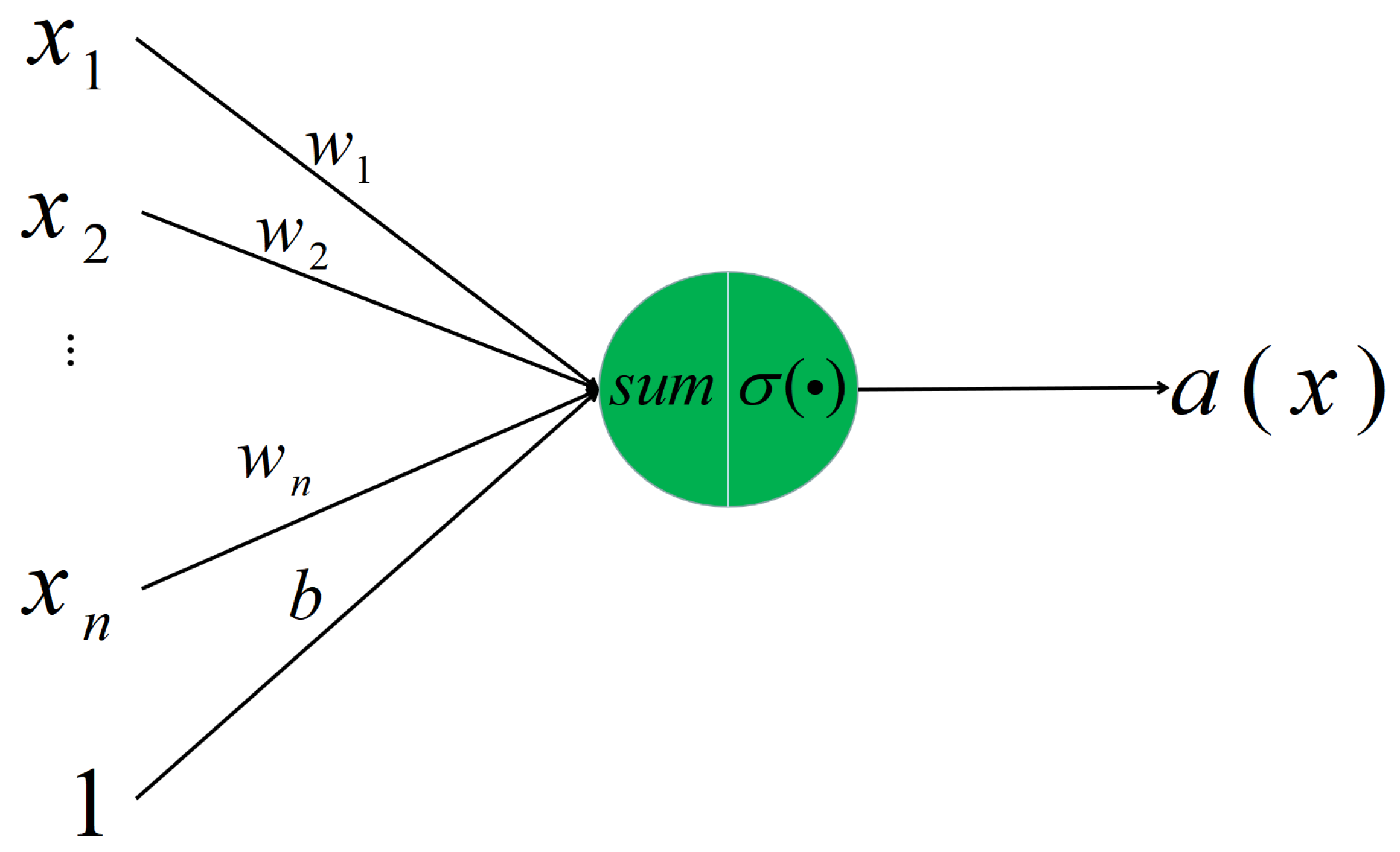
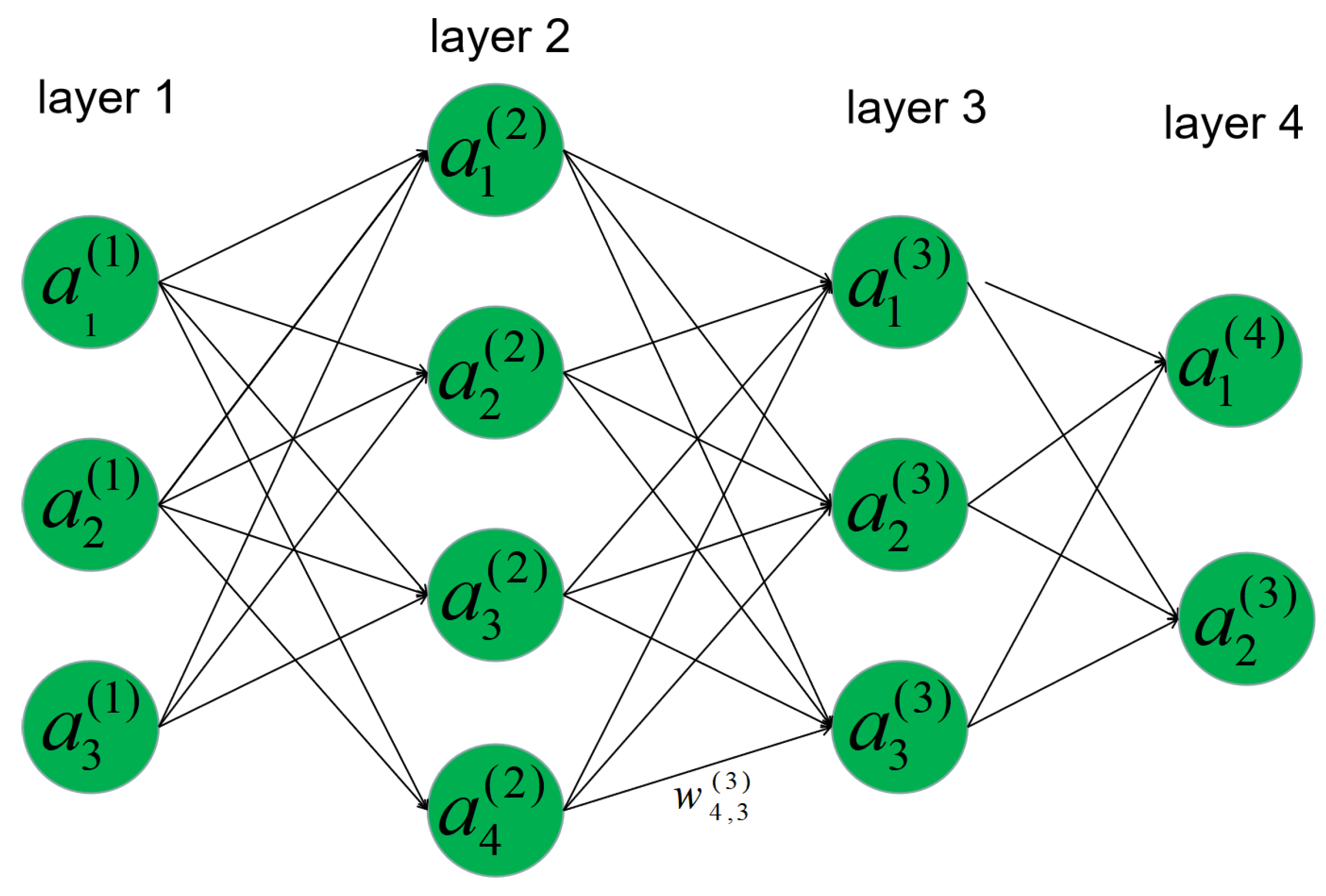
3.1. Multilayer Perceptron
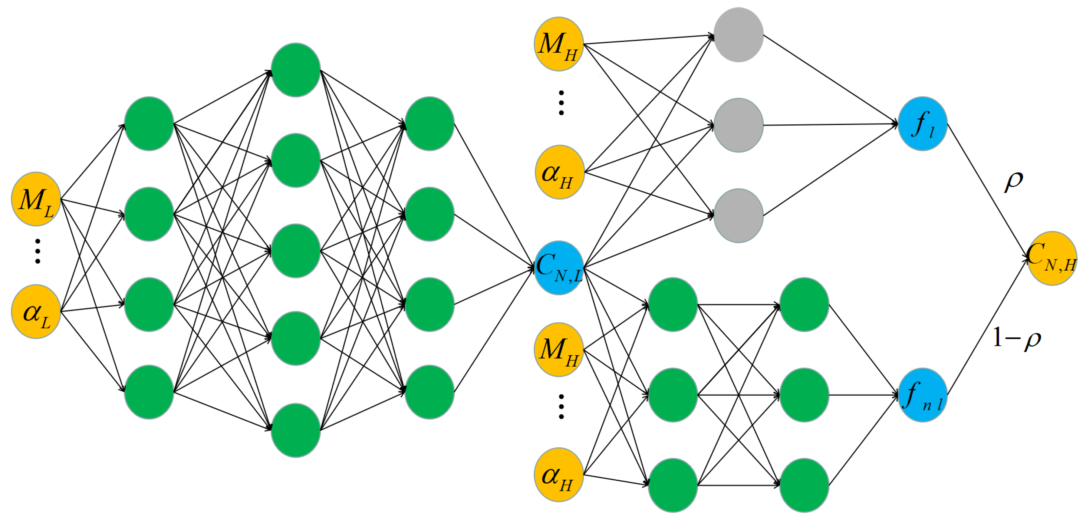
3.2. Multi-Fidelity Aerodynamic Data Fusion with Deep Neural Networks
4. Results and Discussion
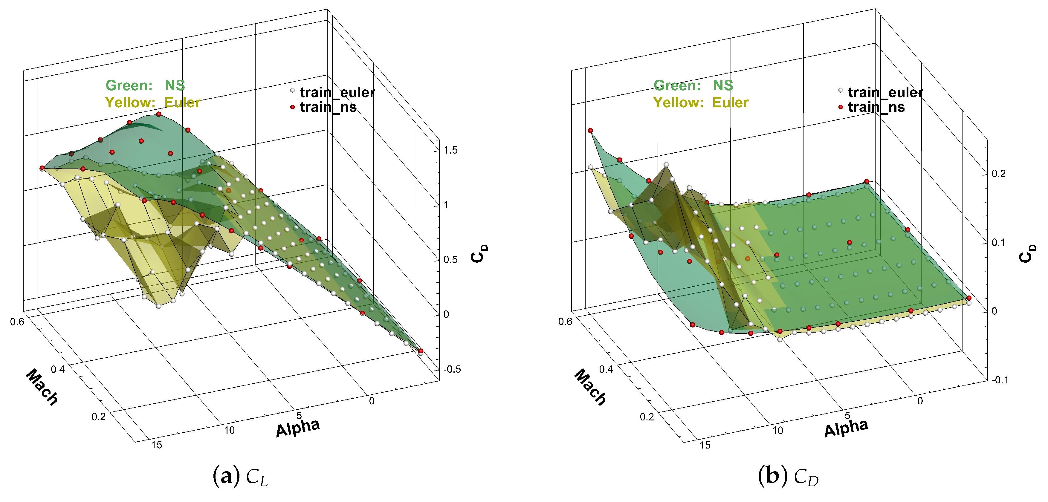
4.1. Data Preparation
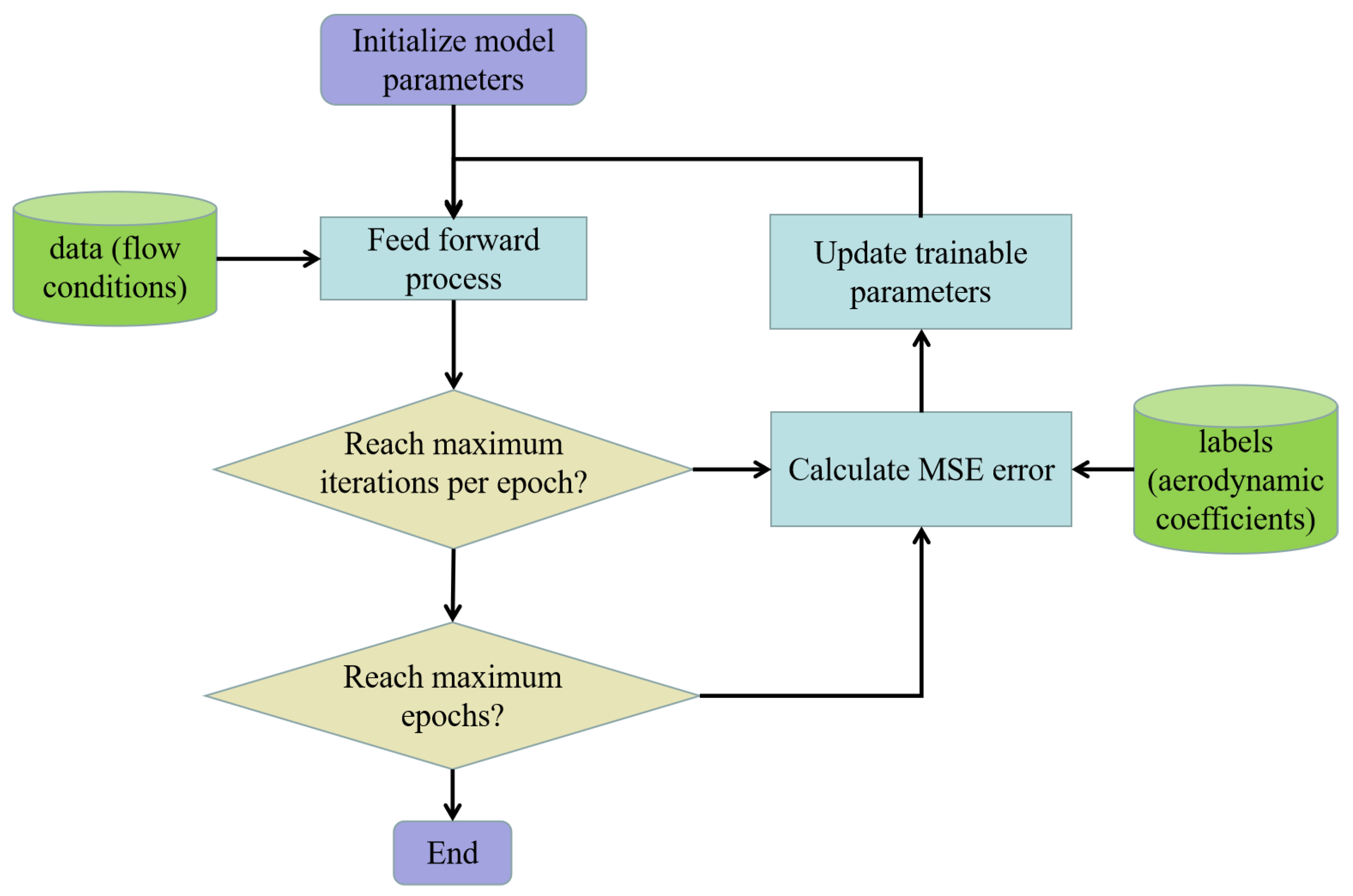
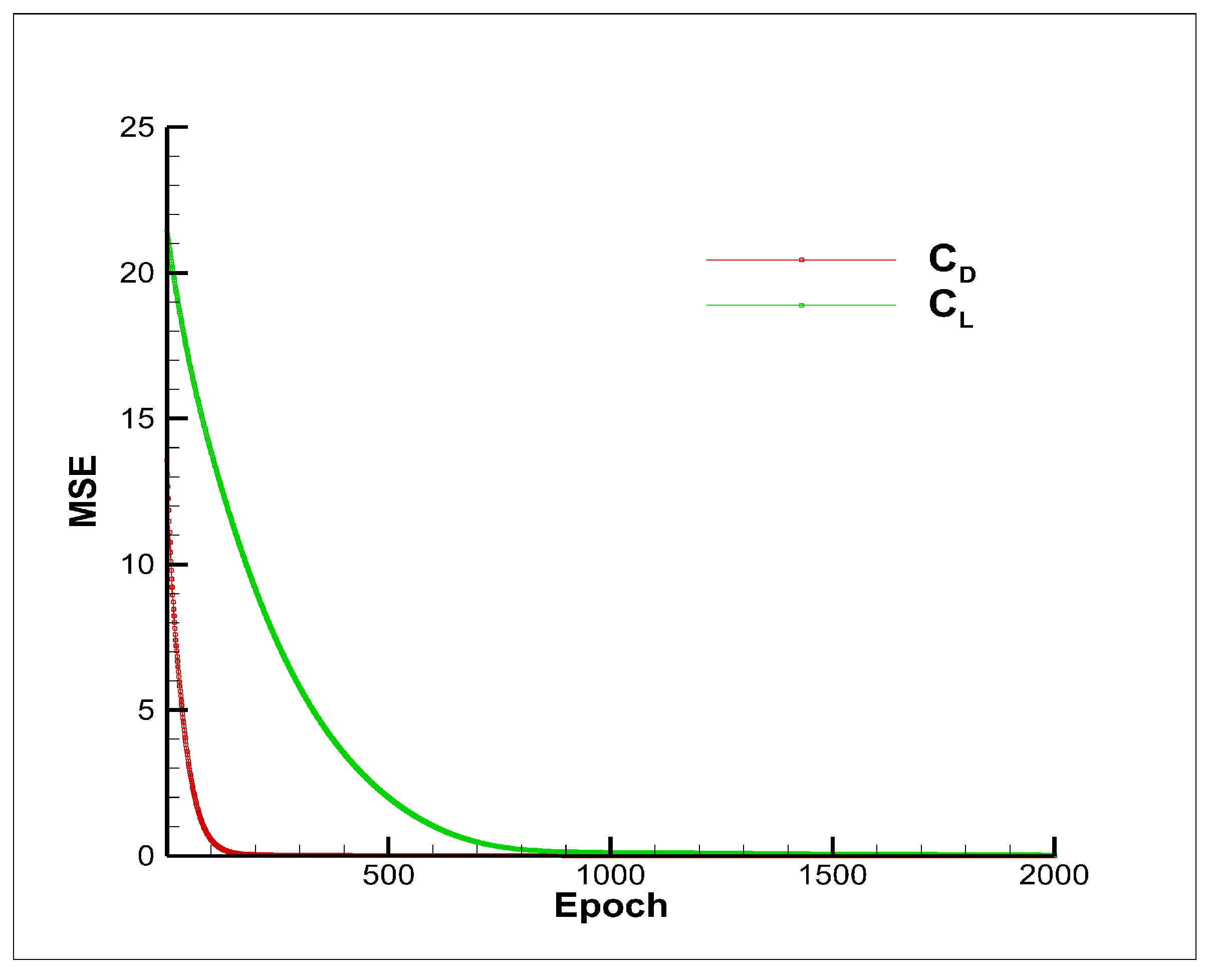
4.2. Model Training
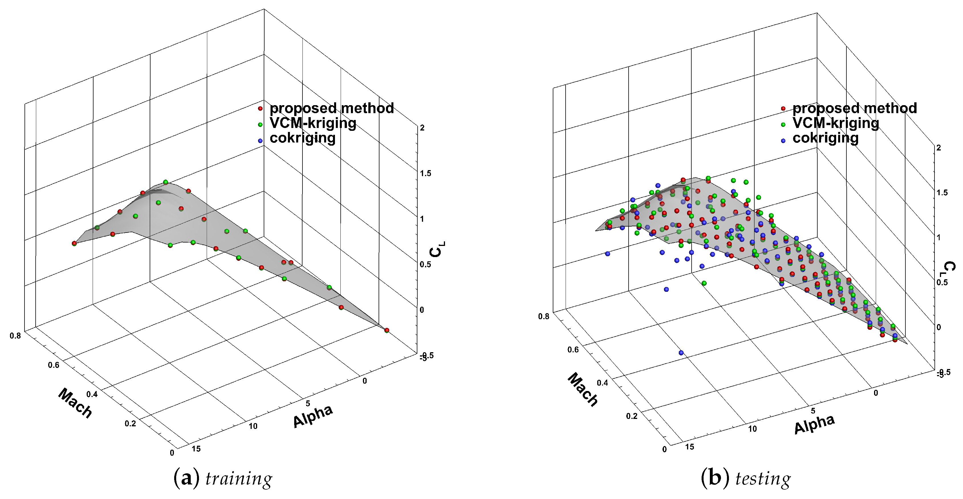
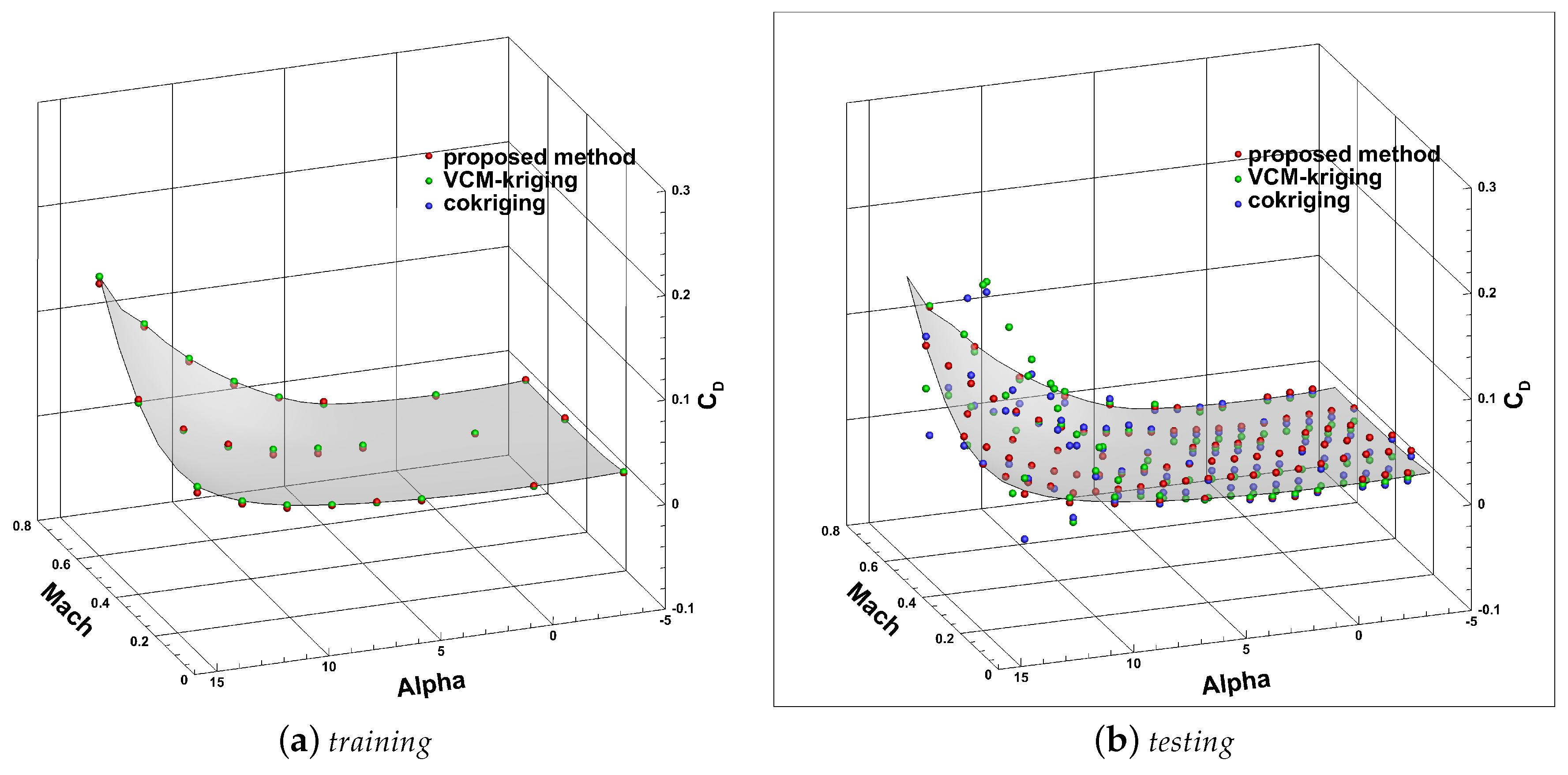
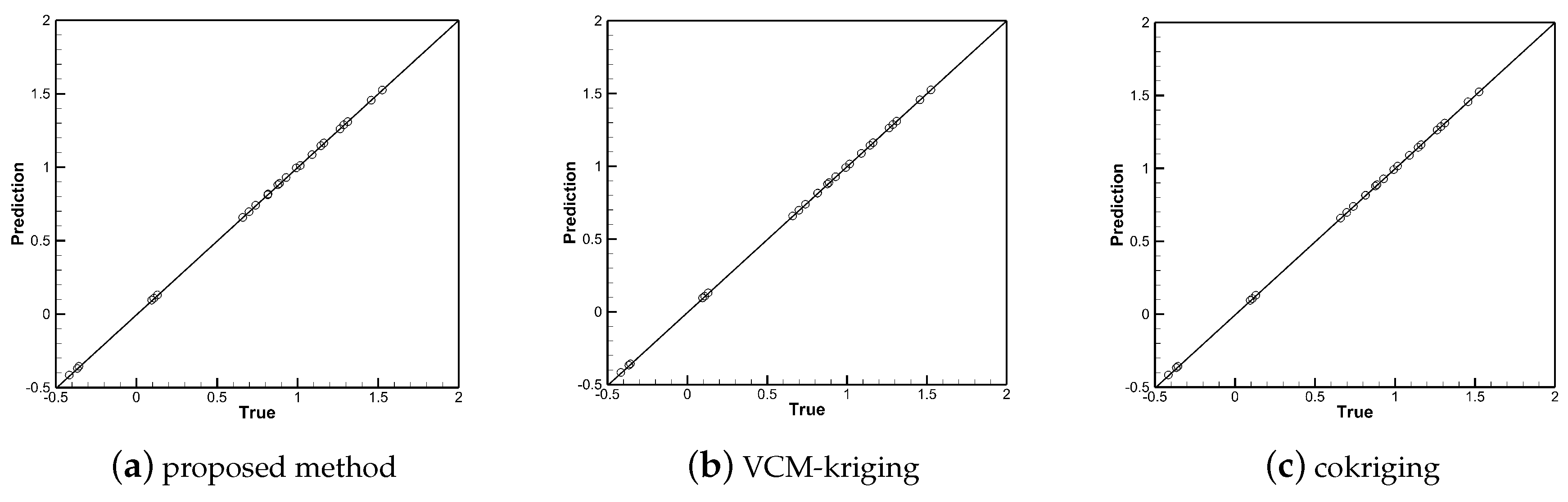
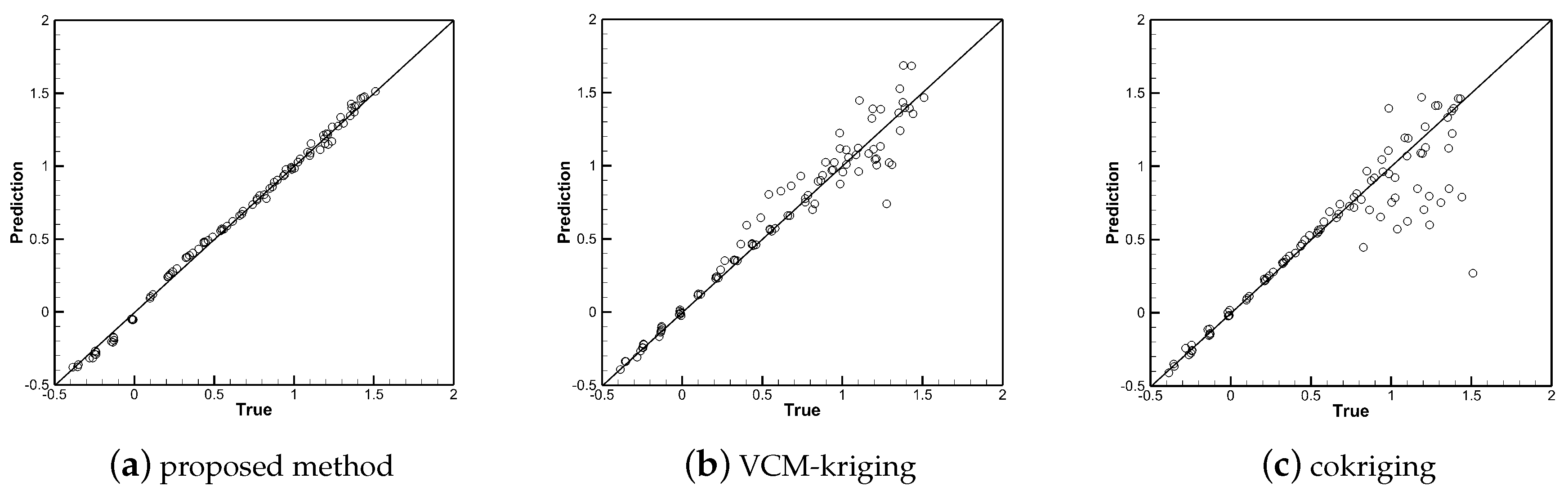
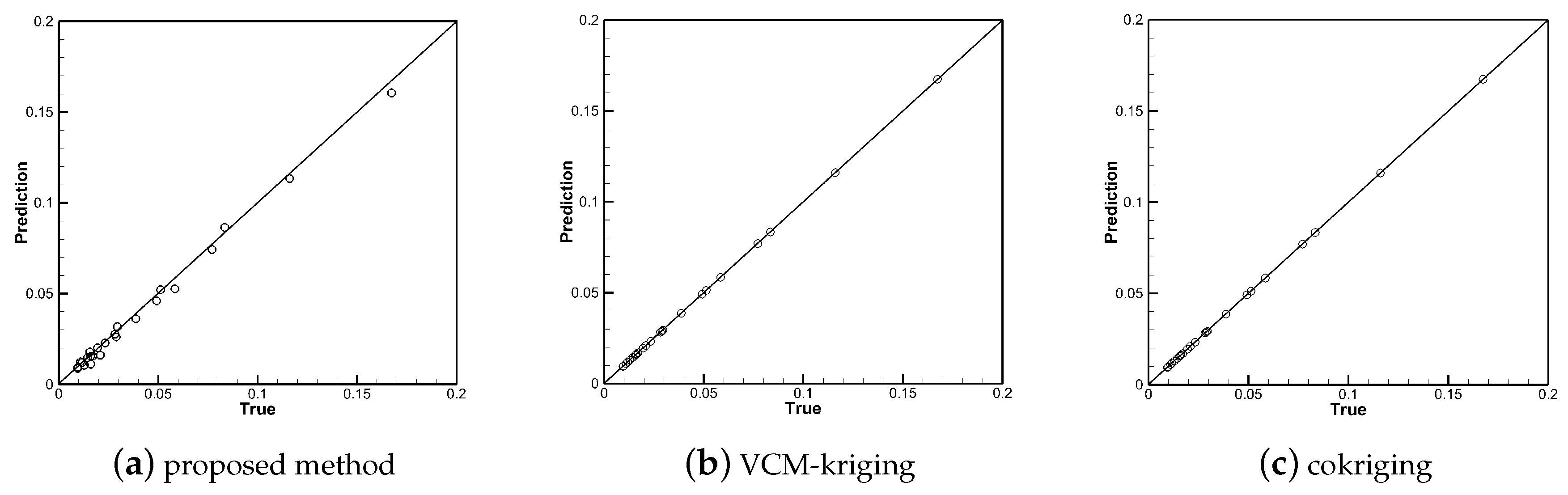
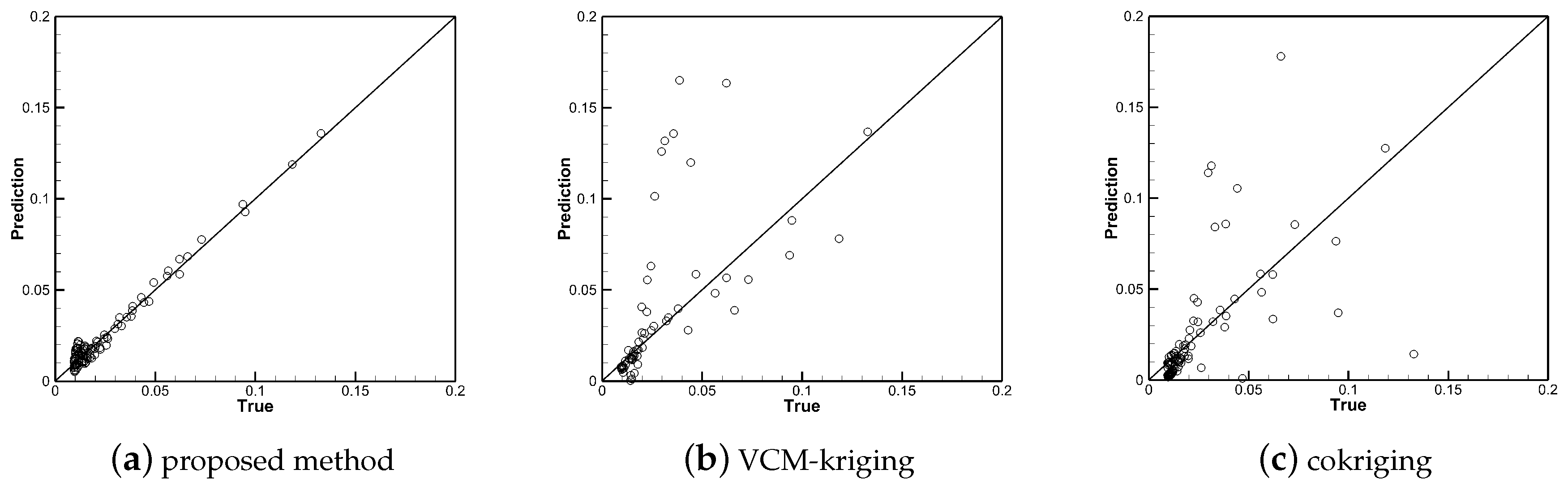
4.3. Discussion
5. Conclusions
Author Contributions
Funding
Conflicts of Interest
References
- Chen, J.; Zhang, Y.; Zhang, Y.; Chen, L. Review of correlation analysis of aerodynamic data between flight and ground prediction for hypersonic vehicle. Acta Aerodyn. Sin. 2014, 32, 587–599. [Google Scholar] [CrossRef]
- Hall, R.M.; Biedron, R.T.; Ball, D.N.; Bogue, D.R.; Chung, J.; Green, B.E.; Grismer, M.J.; Brooks, G.P.; Chambers, J.R. Computational Methods for Stability and Control (COMSAC): The Time Has Come. AIAA J. 2005. [Google Scholar] [CrossRef]
- Kuya, Y.; Takeda, K.; Zhang, X. Optimal Surrogate Modelling Approaches for Combining Experimental and Computational Fluid Dynamics Datasets. In Proceedings of the 50th AIAA/ASME/ASCE/AHS/ASC Structures, Structural Dynamics, and Materials Conference, Palm Springs, CA, USA, 4–7 May 2009; p. 2216. [Google Scholar]
- Kaifeng, H.E.; Qian, W.; Wang, Q.; Kong, Y.; Wang, W. Application of data fusion technique in aerodynamics studies. Acta Aerodyn. Sin. 2014, 32, 777–782. [Google Scholar]
- Zheng, J.; Shao, X.; Liang, G.; Ping, J.; Li, Z. A hybrid variable-fidelity global approximation modelling method combining tuned radial basis function base and kriging correction. J. Eng. Des. 2013, 24, 604–622. [Google Scholar] [CrossRef]
- Rosenbaum, B.; Schulz, V. Comparing sampling strategies for aerodynamic Kriging surrogate models. ZAMM J. Appl. Math. Mech. 2012, 92, 852–868. [Google Scholar] [CrossRef]
- Queipo, N.V.; Haftka, R.T.; Shyy, W.; Goel, T.; Vaidyanathan, R.; Tucker, P.K. Surrogate-based analysis and optimization. Prog. Aerosp. Sci. 2005, 41, 1–28. [Google Scholar] [CrossRef]
- Ai, Y. Research on Response Surface Method Optimisation Based on Radial Basis Function. Master’s Thesis, Huazhong University of Science and Technology, Wuhan, China, 2012. [Google Scholar]
- Barton, R.R. Simulation optimization using metamodels. In Proceedings of the 2009 Winter Simulation Conference (WSC), Austin, TX, USA, 13–16 December 2009; pp. 230–238. [Google Scholar]
- Younis, A.; Dong, Z. Trends, features, and tests of common and recently introduced global optimization methods. Eng. Optim. 2010, 42, 691–718. [Google Scholar] [CrossRef]
- Laurenceau, J.; Sagaut, P. Building Ecien t Response Surfaces of Aerodynamic Functions with Kriging and Cokriging. AIAA J. 2008, 46, 498–507. [Google Scholar] [CrossRef]
- Forrester, A.; Sobester, A.; Keane, A. Engineering Design via Surrogate Modelling: A Practical Guide; John Wiley & Sons: Chichester, UK, 2008. [Google Scholar]
- Chen, V.C.P.; Tsui, K.; Barton, R.R.; Meckesheimer, M. A review on design, modeling and applications of computer experiments. IIE Trans. 2006, 38, 273–291. [Google Scholar] [CrossRef]
- Santner, T.J.; Williams, B.J.; Notz, W.; Williams, B.J. The Design and Analysis of Computer Experiments; Springer: New York, NY, USA, 2003; Volume 1. [Google Scholar]
- Park, C.; Haftka, R.T.; Kim, N.H. Remarks on multi-fidelity surrogates. Struct. Multidiscip. Optim. 2017, 55, 1029–1050. [Google Scholar] [CrossRef]
- Perdikaris, P.; Raissi, M.; Damianou, A.; Lawrence, N.D.; Karniadakis, G.E. Nonlinear information fusion algorithms for data-efficient multi-fidelity modelling. Proc. Math. Phys. Eng. Sci. 2017, 473, 20160751. [Google Scholar] [CrossRef] [PubMed]
- Meng, X.; Karniadakis, G.E. A composite neural network that learns from multi-fidelity data: Application to function approximation and inverse PDE problems. J. Comput. Phys. 2020, 401, 109020. [Google Scholar] [CrossRef]
- Hutchison, M.; Mason, W.; Grossman, B.; Haftka, R. Aerodynamic Optimization of an HSCT Configuration Using Variable-Complexity Modeling. In Proceedings of the 31st Aerospace Sciences Meeting, Reno, NV, USA, 11 January 1993. [Google Scholar] [CrossRef]
- Hutchison, M.G.; Unger, E.R.; Mason, W.H.; Grossman, B.; Haftka, R.T. Variable-complexity aerodynamic optimization of a high-speed civil transport wing. J. Aircr. 1994, 31, 110–116. [Google Scholar] [CrossRef]
- Keane, A.J. Wing Optimization Using Design of Experiment, Response Surface, and Data Fusion Methods. J. Aircr. 2003, 40, 741–750. [Google Scholar] [CrossRef]
- Leary, S.J.; Bhaskar, A.; Keane, A.J. A Knowledge-Based Approach To Response Surface Modelling in Multifidelity Optimization. J. Glob. Optim. 2003, 26, 297–319. [Google Scholar] [CrossRef]
- Tang, C.; Gee, K.; Lawrence, S. Generation of aerodynamic data using a design of experiment and data fusion approach. In Proceedings of the 43rd AIAA Aerospace Sciences Meeting and Exhibit, Reno, NV, USA, 10–13 January 2005; p. 1137. [Google Scholar]
- Tyan, M.; Kim, M.; Pham, V.; Choi, C.K.; Nguyen, T.L.; Lee, J.W. Development of Advanced Aerodynamic Data Fusion Techniques for Flight Simulation Database Construction. In Proceedings of the 2018 Modeling and Simulation Technologies Conference, Atlanta, GA, USA, 25–29 June 2018. [Google Scholar]
- Renganathan, A.; Harada, K.; Mavris, D.N. Multifidelity Data Fusion via Bayesian Inference. In Proceedings of the AIAA Aviation 2019 Forum, Dallas, TX, USA, 17–21 June 2019. [Google Scholar]
- Ghoreyshi, M.; Badcock, K.J.; Woodgate, M.A. Accelerating the Numerical Generation of Aerodynamic Models for Flight Simulation. J. Aircr. 2009, 46, 972–980. [Google Scholar] [CrossRef]
- Kuya, Y.; Takeda, K.; Xin, Z.; Forrester, A.I.J. Multifidelity Surrogate Modeling of Experimental and Computational Aerodynamic Data Sets. AIAA J. 2011, 49, 289–298. [Google Scholar] [CrossRef]
- Zhang, Q. Development of a Data Fusion Framework for the Aerodynamic Analysis of Launchers. Master’s Thesis, Delft University of Technology, Delft, The Netherlands, 2017. [Google Scholar]
- Unger, E.R.; Hutchinson, M.G.; Rais-Rohani, M.; Haftka, R.T.; Grossman, B. Variable-Complexity Design of a Transport Wing. Int. J. Syst. Autom. Res. Appl. 1992, 2, 87–113. [Google Scholar]
- Knill, D.; Giunta, A.; Baker, C.; Grossman, B.; Mason, W.; Haftka, R.; Watson, L. HSCT Configuration Design Using Response Surface Approximations of Supersonic Euler Aerodynamics. In Proceedings of the 36th AIAA Aerospace Sciences Meeting and Exhibit, Reno, NV, USA, 12–15 January 1998. [Google Scholar] [CrossRef]
- Baker, C.A.; Grossman, B.; Haftka, R.T.; Mason, W.H.; Watson, L.T. High-speed civil transport design space exploration using aerodynamic response surface approximations. J. Aircr. 2002, 39, 215–220. [Google Scholar] [CrossRef]
- Han, Z. Kriging surrogate model and its application to design optimization: A review of recent progress. Acta Aeronaut. Astronaut. Sin. 2016, 37, 3197–3225. [Google Scholar]
- Forrester, A.I.; SÃbester, A.; Keane, A.J. Multi-fidelity optimization via surrogate modelling. Proc. R. Soc. Math. Phys. Eng. Sci. 2007, 463, 3251–3269. [Google Scholar] [CrossRef]
- Santos, M.; Mattos, B.; Girardi, R. Aerodynamic Coefficient Prediction of Airfoils Using Neural Networks. In Proceedings of the AIAA Aerospace Sciences Meeting & Exhibit, Reno, NV, USA, 7–10 January 2008. [Google Scholar]
- Sekar, V.; Zhang, M.; Shu, C.; Khoo, B.C. Inverse Design of Airfoil Using a Deep Convolutional Neural Network. AIAA J. 2019, 57, 993–1003. [Google Scholar] [CrossRef]
- Rumelhart, D.E.; Hinton, G.E.; Williams, R.J. Learning Representations by Back Propagating Errors. Nature 1986, 323, 533–536. [Google Scholar] [CrossRef]
- Babaee, H.; Perdikaris, P.; Chryssostomidis, C.; Karniadakis, G.E. Multi-fidelity modelling of mixed convection based on experimental correlations and numerical simulations. J. Fluid Mech. 2016, 809, 895–917. [Google Scholar] [CrossRef]
- Kingma, D.; Ba, J. Adam: A Method for Stochastic Optimization. arXiv 2014, arXiv:1412.6980. [Google Scholar]
- Ruder, S. An overview of gradient descent optimization algorithms. arXiv 2016, arXiv:1609.04747. [Google Scholar]
- Wang, J.J.; Gao, Z.H. Analysis and Improvement of HicksHenne Airfoil Parameterization Method. Aeronaut. Comput. Tech. 2010, 40, 47–49. [Google Scholar]
- Wang, J.; Yi, X.; Xiao, Z. Numerical simulation of ice shedding from ARJ21-700. Acta Aerodyn. Sin. 2013, 31, 430–436. [Google Scholar]
- Chen, K.; Huang, D.; Li, Y. Grid convergence study in the resistance calculation of a trimaran. J. Mar. Sci. Appl. 2008, 7, 174–178. [Google Scholar] [CrossRef]


| Grid | (%) | (%) | ||||
|---|---|---|---|---|---|---|
| gird1 () | 0.01088 | 9.46 | 0.42 | 0.34306 | 1.2 | 0.53 |
| gird1 () | 0.01028 | 3.42 | 0.34443 | 0.8 | ||
| gird1 () | 0.01003 | 0.9 | 0.34516 | 0.6 | ||
| gird1 () | 0.00994 | - | - | 0.34740 | - | - |
| Time | Coefficient | Proposed Method | Variable Complexity Modeling (VCM)-Kriging | Cokriging |
|---|---|---|---|---|
| Training time | 204 s | 53 s | 61 s | |
| 201 s | 50 s | 60 s | ||
| Prediction time | <1 s | <1 s | <1 s | |
| <1 s | <1 s | <1 s |
| Set | Method | Root Mean Square Error (RMSE) | |||
|---|---|---|---|---|---|
| train | proposed method | 0.0024 | 0.0029 | 0.0023 | 0.0584 |
| VCM-kriging | 0.0 | 0.0 | 0.0 | 0.0 | |
| cokriging | 0.0 | 0.0 | 0.0 | 0.0 | |
| test | proposed method | 0.0333 | 0.0038 | 0.0389 | 0.1289 |
| VCM-kriging | 0.1220 | 0.0382 | 0.1110 | 0.8298 | |
| cokriging | 0.2240 | 0.0296 | 0.1627 | 0.5840 | |
© 2020 by the authors. Licensee MDPI, Basel, Switzerland. This article is an open access article distributed under the terms and conditions of the Creative Commons Attribution (CC BY) license (http://creativecommons.org/licenses/by/4.0/).
Share and Cite
He, L.; Qian, W.; Zhao, T.; Wang, Q. Multi-Fidelity Aerodynamic Data Fusion with a Deep Neural Network Modeling Method. Entropy 2020, 22, 1022. https://doi.org/10.3390/e22091022
He L, Qian W, Zhao T, Wang Q. Multi-Fidelity Aerodynamic Data Fusion with a Deep Neural Network Modeling Method. Entropy. 2020; 22(9):1022. https://doi.org/10.3390/e22091022
Chicago/Turabian StyleHe, Lei, Weiqi Qian, Tun Zhao, and Qing Wang. 2020. "Multi-Fidelity Aerodynamic Data Fusion with a Deep Neural Network Modeling Method" Entropy 22, no. 9: 1022. https://doi.org/10.3390/e22091022
APA StyleHe, L., Qian, W., Zhao, T., & Wang, Q. (2020). Multi-Fidelity Aerodynamic Data Fusion with a Deep Neural Network Modeling Method. Entropy, 22(9), 1022. https://doi.org/10.3390/e22091022