All articles published by MDPI are made immediately available worldwide under an open access license. No special
permission is required to reuse all or part of the article published by MDPI, including figures and tables. For
articles published under an open access Creative Common CC BY license, any part of the article may be reused without
permission provided that the original article is clearly cited. For more information, please refer to
https://www.mdpi.com/openaccess.
Feature papers represent the most advanced research with significant potential for high impact in the field. A Feature
Paper should be a substantial original Article that involves several techniques or approaches, provides an outlook for
future research directions and describes possible research applications.
Feature papers are submitted upon individual invitation or recommendation by the scientific editors and must receive
positive feedback from the reviewers.
Editor’s Choice articles are based on recommendations by the scientific editors of MDPI journals from around the world.
Editors select a small number of articles recently published in the journal that they believe will be particularly
interesting to readers, or important in the respective research area. The aim is to provide a snapshot of some of the
most exciting work published in the various research areas of the journal.
We compute exact values respectively bounds of dissimilarity/distinguishability measures–in the sense of the Kullback-Leibler information distance (relative entropy) and some transforms of more general power divergences and Renyi divergences–between two competing discrete-time Galton-Watson branching processes with immigration GWI for which the offspring as well as the immigration (importation) is arbitrarily Poisson-distributed; especially, we allow for arbitrary type of extinction-concerning criticality and thus for non-stationarity. We apply this to optimal decision making in the context of the spread of potentially pandemic infectious diseases (such as e.g., the current COVID-19 pandemic), e.g., covering different levels of dangerousness and different kinds of intervention/mitigation strategies. Asymptotic distinguishability behaviour and diffusion limits are investigated, too.
(This paper is a thoroughly revised, extended and retitled version of the preprint arXiv:1005.3758v1 of both authors) Over the past twenty years, density-based divergences –also known as (dis)similarity measures, directed distances, disparities, distinguishability measures, proximity measures–between probability distributions P and Q, have turned out to be of substantial importance for decisive statistical tasks such as parameter estimation, testing for goodness-of-fit, Bayesian decision procedures, change-point detection, clustering, as well as for other research fields such as information theory, artificial intelligence, machine learning, signal processing (including image and speech processing), pattern recognition, econometrics, and statistical physics. For some comprehensive overviews on the divergence approach to statistics and probability, the reader is referred to the insightful books of e.g., Liese & Vajda [1], Read & Cressie [2], Vajda [3], Csiszár & Shields [4], Stummer [5], Pardo [6], Liese & Miescke [7], Basu et al. [8], Voinov et al. [9], the survey articles of e.g., Liese & Vajda [10], Vajda & van der Meulen [11], the structure-building papers of Stummer & Vajda [12], Kißlinger & Stummer [13] and Broniatowski & Stummer [14], and the references therein. Divergence-based bounds of minimal mean decision risks (e.g., Bayes risks in finance) can be found e.g., in Stummer & Vajda [15] and Stummer & Lao [16].
Amongst the above-mentioned dissimilarity measures, an important omnipresent subclass are the so-called divergences of Csiszar [17], Ali & Silvey [18] and Morimoto [19]; important special cases thereof are the total variation distance and the very frequently used order power divergences (also known as alpha-entropies, Cressie-Read measures, Tsallis cross-entropies) with . The latter cover e.g., the very prominent Kullback-Leibler information divergence (also called relative entropy), the (squared) Hellinger distance , as well as the Pearson chi-square divergence . It is well known that the power divergences can be build with the help of the order Hellinger integrals (where e.g., the case corresponds to the well-known Bhattacharyya coefficient), which are information measures of interest by their own and which are also the crucial ingredients of order Renyi divergences (see e.g., Liese & Vajda [1], van Erven & Harremoes [20]); the case corresponds to the well-known Bhattacharyya distance.
The above-mentioned information/dissimilarity measures have been also investigated in non-static, time-dynamic frameworks such as for various different contexts of stochastic processes like processes with independent increments (see e.g., Newman [21], Liese [22], Memin & Shiryaev [23], Jacod & Shiryaev [24], Liese & Vajda [1], Linkov & Shevlyakov [25]), Poisson point processes (see e.g., Liese [26], Jacod & Shiryaev [24], Liese & Vajda [1]), diffusion prcoesses and solutions of stochastic differential equations with continuous paths (see e.g., Kabanov et al. [27], Liese [28], Jacod & Shiryaev [24], Liese & Vajda [1], Vajda [29], Stummer [30,31,32], Stummer & Vajda [15]), and generalized binomial processes (see e.g., Stummer & Lao [16]); further related literature can be found e.g., in references of the aforementioned papers and books.
Another important class of time-dynamic models is given by discrete-time integer-valued branching processes, in particular (Bienaymé-)Galton-Watson processes without immigration GW respectively with immigration (resp. importation, invasion) GWI, which have numerous applications in biotechnology, population genetics, internet traffic research, clinical trials, asset price modelling, derivative pricing, and many others. As far as important terminology is concerned, we abbreviatingly subsume both models as GW(I) and, simply as GWI in case that GW appears as a parameter-special-case of GWI; recall that a GW(I) is called subcritical respectively critical respectively supercritical if its offspring mean is less than 1 respectively equal to 1 respectively larger than 1.
For applications of GW(I) in epidemiology, see e.g., the works of Bartoszynski [33], Ludwig [34], Becker [35,36], Metz [37], Heyde [38], von Bahr & Martin-Löf [39], Ball [40], Jacob [41], Barbour & Reinert [42], Section 1.2 of Britton & Pardoux [43]); for more details see Section 2.3 below.
For connections of GW(I) to time series of counts including GLM models, see e.g., Dion, Gauthier & Latour [44], Grunwald et al. [45], Kedem & Fokianos [46], Held, Höhle & Hofmann [47], and Weiß [48]; a more comprehensive discussion can be found in Section 2.2 below.
As far as the combined study of information measures and GW processes is concerned, let us first mention that (transforms of) power divergences have been used for supercritical Galton-Watson processes without immigration for instance as follows: Feigin & Passy [49] study the problem to find an offspring distribution which is closest (in terms of relative entropy type distance) to the original offspring distribution and under which ultimate extinction is certain. Furthermore, Mordecki [50] gives an equivalent characterization for the stable convergence of the corresponding log-likelihood process to a mixed Gaussian limit, in terms of conditions on Hellinger integrals of the involved offspring laws. Moreover, Sriram & Vidyashankar [51] study the properties of offspring-distribution-parameters which minimize the squared Hellinger distance between the model offspring distribution and the corresponding non-parametric maximum likelihood estimator of Guttorp [52]. For the setup of GWI with Poisson offspring and nonstochastic immigration of constant value 1, Linkov & Lunyova [53] investigate the asymptotics of Hellinger integrals in order to deduce large deviation assertions in hypotheses testing problems.
In contrast to the above-mentioned contexts, this paper pursues the following main goals:
(MG1)
for any time horizon and any criticality scenario (allowing for non-stationarities), to compute lower and upper bounds–and sometimes even exact values–of the Hellinger integrals , power divergences and Renyi divergences of two alternative Galton-Watson branching processes and (on path/scenario space), where (i) has Poisson() distributed offspring as well as Poisson() distributed immigration, and (ii) has Poisson() distributed offspring as well as Poisson() distributed immigration; the non-immigration cases are covered as ; as a side effect, we also aim for corresponding asymptotic distinguishability results;
(MG2)
to compute the corresponding limit quantities for the context in which (a proper rescaling of) the two alternative Galton-Watson processes with immigration converge to Feller-type branching diffusion processes, as the time-lags between the generation-size observations tend to zero;
(MG3)
as an exemplary field of application, to indicate how to use the results of (MG1) for Bayesian decision making in the epidemiological context of an infectious-disease pandemic (e.g., the current COVID-19), where e.g., potential state-budgetary losses can be controlled by alternative public policies (such as e.g., different degrees of lockdown) for mitigations of the time-evolution of the number of infectious persons (being quantified by a GW(I)). Corresponding Neyman-Pearson testing will be treated, too.
Because of the involved Poisson distributions, these goals can be tackled with a high degree of tractability, which is worked out in detail with the following structure (see also the full table of contents after this paragraph): in Section 2, we first introduce (i) the basic ingredients of Galton-Watson processes together with their interpretations in the above-mentioned pandemic setup where it is essential to study all types of criticality (being connected with levels of reproduction numbers), (ii) the employed fundamental information measures such as Hellinger integrals, power divergences and Renyi divergences, (iii) the underlying decision-making framework, as well as (iv) connections to time series of counts and asymptotical distinguishability. Thereafter, we start our detailed technical analyses by giving recursive exact values respectively recursive bounds–as well as their applications–of Hellinger integrals (see Section 3), power divergences and Renyi divergences (see Section 4 and Section 5). Explicit closed-form bounds of Hellinger integrals will be worked out in Section 6, whereas Section 7 deals with Hellinger integrals and power divergences of the above-mentioned Galton-Watson type diffusion approximations.
2. The Framework and Application Setups
2.1. Process Setup
We investigate dissimilarity measures and apply them to decisions, in the following context. Let the integer-valued random variable () denote the size of the nth generation of a population (of persons, organisms, spreading news, other kind of objects, etc.) with specified characteristics, and suppose that for the modelling of the time-evolution we have the choice between the following two (e.g., alternative, competing) models and :
a discrete-time homogeneous Galton-Watson process with immigration GWI, given by the recursive description
where is the number of offspring of the kth object (e.g., organism, person) within the th generation, and denotes the number of immigrating objects in the nth generation. Notice that we employ an arbitrary deterministic (i.e., degenerate random) initial generation size . We always assume that under the corresponding dynamics-governing law
(GWI1)
the collection consists of independent and identically distributed (i.i.d.) random variables which are Poisson distributed with parameter ,
(GWI2)
the collection consists of i.i.d. random variables which are Poisson distributed with parameter (where stands for the degenerate case of having no immigration),
(GWI3)
Y and are independent.
a discrete-time homogeneous Galton-Watson process with immigration GWI given by the same recursive description (1), but with different dynamics-governing law under which (GWI1) holds with parameter (instead of ), (GWI2) holds with (instead of ), and (GWI3) holds. As a side remark, in some contexts the two models and may function as a “sandwich” of a more complicated not fully known model.
Basic and advanced facts on general GWI (introduced by Heathcote [54]) can be found e.g., in the monographs of Athreya & Ney [55], Jagers [56], Asmussen & Hering [57], Haccou [58]; see also e.g., Heyde & Seneta [59], Basawa & Rao [60], Basawa & Scott [61], Sankaranarayanan [62], Wei & Winnicki [63], Winnicki [64], Guttorp [52] as well as Yanev [65] (and also the references therein all those) for adjacent fundamental statistical issues including the involved technical and conceptual challenges.
For the sake of brevity, wherever we introduce or discuss corresponding quantities simultaneously for both models and , we will use the subscript • as a synonym for either the symbol or . For illustration, recall the well-known fact that the corresponding conditional probabilities
are again Poisson-distributed, with parameter .
In oder to achieve a transparently representable structure of our results, we subsume the involved parameters as follows:
(PS1)
is the set of all constellations of real-valued parameters , , , , such that or (or both); in other words, both models are non-identical and have non-vanishing immigration;
(PS2)
is the set of all of real-valued parameters , , , such that ; this corresponds to the important special case that both models have no immigration and are non-identical;
(PS3)
the resulting disjoint union will be denoted by .
Notice that for (unbridgeable) technical reasons, we do not allow for “crossovers” between “immigration and no-immigration” (i.e., and , respectively, and ). For practice, this is not a strong restriction, since one may take e.g., and .
For the non-immigration case one has the following extinction properties (see e.g., Harris [66], Athreya & Ney [55]). As usual, let us define the extinction time for all integers if this minimum exists, and else. Correspondingly, let be the extinction set. If the offspring mean satisfies —which is called the subcritical case– or —which is known as the critical case–then extinction is certain, i.e., there holds . However, if the offspring mean satisfies —which is called the supercritical case–then there is a probability greater than zero, that the population never dies out, i.e., . In the latter case, explodes (a.s.) to infinity as .
In contrast, for the (nondegenerate, nonvanishing) immigration case there is no extinction, viz. , although there may be zero population for some intermediate time ; but due to the immigration, with probability one there is always a later time , such that . Nevertheless, also for the setup it is important to know whether —which is still called (super-, sub-)criticality–since e.g., in the case the population size converges (as ) to a stationary distribution on whereas for the behaviour is non-stationary (non-ergodic), see e.g., Athreya & Ney [55].
At this point, let us emphasize that in our investigations (both for and for ) we do allow for “crossovers” between “different criticalities”, i.e., we deal with all cases versus all cases ; as will be explained in the following, this unifying flexibility is especially important for corresponding epidemiological-model comparisons (e.g., for the sake of decision making).
One of our main goals is to quantitatively compare (the time-evolution of) two competing GWI models and with respective parameter sets and , in terms of the information measures (Hellinger intergrals), (power divergences), (Renyi divergences). The latter two express a distance (degree of dissimilarity) between and . From this, we shall particularly derive applications for decision making under uncertainty (including tests).
2.2. Connections to Time Series of Counts
It is well known that a Galton-Watson process with Poisson offspring (with parameter ) and Poisson immigration (with parameter ) is “distributionally” equal to each of the following models (listed in “tree-type” chronological order):
(M1)
a Poissonian Generalized Integer-valued Autoregressive process GINAR(1) in the sense of Gauthier & Latour [67] (see also Dion, Gauthier & Latour [44], Latour [68], as well as Grunwald et al. [45]), that is, a first-order autoregressive times series with Poissonian thinning (with parameter ) and Poissonian innovations (with parameter );
(M2)
Poissonian first order Conditional Linear Autoregressive model (Poissonian CLAR(1)) in the sense of Grunwald et al. [45] (and earlier preprints thereof) (since the conditional expectation is
); this can be equally seen as Poissonian autoregressive Generalized Linear Model GLM with identity link function (cf. [45] as well as Chapter 4 of Kedem & Fokianos [46]), that is, an autoregressive GLM with Poisson distribution as random component and the identity link as systematic component;
the same model was used (and generalized)
(M2i)
under the name BIN(1) by Rydberg & Shephard [69] for the description of the number of stock transactions/trades recorded up to time n;
(M2ii)
under the name Poisson autoregressive model PAR(1) by Brandt & Williams [70] for the description of event counts in political and other social science applications;
(M2iii)
under the name Autoregressive Conditional Poisson model ACP(1,0) by Heinen [71];
(M2iv)
by Held, Höhle & Hofmann [47] as well as Held et al. [72], as a description of the time-evolution of counts from infectious disease surveillance databases, where (respectively, ) is interpreted as driving parameter of epidemic (respectively, endemic) component; in principle, this type of modelling can be also implicitly recovered as a special case of the epidemics-treating work of Finkenstädt, Bjornstad & Grenfell [73], by assuming trend- and season-neglecting (e.g., intra-year) measles data in urban areas of about 10 million people (provided that their population size approximation extends linearly);
(M2v)
under the name integer-valued Generalized Autoregressive Conditional Heteroscedastic model INGARCH(1,0) by Ferland, Latour & Oraichi [74] (since the conditional variance is ), see also Weiß [75]; this has been refinely named as INARCH(1) model by Weiß [76,77], and frequently applied thereafter; for an “overlapping-generation type” interpretation of the INARCH(1) model, which is an adequate description for the time-evolution of overdispersed counts with an autoregressive serial dependence structure, see Weiß & Testik [78]; for a corresponding comprehensive recent survey (also to more general count time series), the reader is referred to the book of Weiß [48];
Moreover, according to the general considerations of Grunwald et al. [45], the Poissonian Galton-Watson model with immigration may possibly be “distributionally equal” to an integer-valued autoregressive model with random coefficient (thinning).
Nowadays, besides the name homogeneous Galton-Watson model with immigration GWI, the name INARCH(1) seems to be the most used one, and we follow this terminology (with emphasis on GWI). Typical features of the above-mentioned models (M1) to (M2v), are the use of as the set of times, and the assumptions as well as , which guarantee stationarity and ergodicity (see above). In contrast, we employ as the set of times, degenerate (and thus, non-equilibrium) starting distribution, and arbitrary as well as . For such a situation, as explained above, we quantitatively compare two competing GWI models and with respective parameter sets and . Since–as can be seen e.g., in (29) below—we basically employ only (conditionally) distributional ingredients, such as the corresponding likelihood ratio (see e.g., (13) to (15), (27) to (29) below), all the results of the Section 3, Section 4, Section 5 and Section 6 can be immediately carried over to the above-mentioned time-series contexts (where we even allow for non-stationarities, in fact we start with a one-point/Dirac distribution); for the sake of brevity, in the rest of the paper this will not be mentioned explicitly anymore.
Notice that a Poissonian GWI as well as all models (M1) and (M2) are–despite of their conditional Poisson law– typically overdispersed since
with equality iff (i.e., if and only if) (NI) and (extinction at with ).
2.3. Applicability to Epidemiology
The above-mentioned framework can be used for any of the numerous fields of applications of discrete-time branching processes, and of the closely related INARCH(1) models. For the sake of brevity, we explain this—as a kind of running-example—in detail for the currently highly important context of the epidemiology of infectious diseases. For insightful non-mathematical introductions to the latter, see e.g., Kaslow & Evans [79], Osterholm & Hedberg [80]; for a first entry as well as overviews on modelling, the reader is referred to e.g., Grassly & Fraser [81], Keeling & Rohani [82], Yan [83,84], Britton [85], Diekmann, Heesterbeek & Britton [86], Cummings & Lessler [87], Just et al. [88], Britton & Giardina [89], Britton & Pardoux [43]. A survey on the particular role of branching processes in epidemiology can be found e.g., in Jacob [41].
Undoubtedly, by nature, the spreading of an infectious disease through a (human, animal, plant) population is a branching process with possible immigration. Indeed, typically one has the following mechanism:
(D1)
at some time –called the time of exposure (moment of infection)—an individual k of a specified population is infected in a wide sense, i.e., entered/invaded/colonized by a number of transmissible disease-causative pathogens (etiologic agents such as viruses, bacteria, protozoans and other parasites, subviruses (e.g., prions and plant viroids), etc.); the individual is then a host (of pathogens);
(D2)
depending on the level of immunity and some other factors, these pathogens may multiply/replicate within the host to an extent (over a threshold number) such that at time some of the pathogens start to leave their host (shedding of pathogens); in other words, the individual k becomes infectious at the time of onset of infectiousness. Ex post, one can then say that the individual became infected in the narrow sense at earlier time and call it a primary case. The time interval is called the latent/latency/pre-infectious period of k, and its duration (in some literature, there is no verbal distinction between them); notice that may differ from the time of onset (first appearance) of symptoms, which leads to the so-called incubation period ; if then is called the pre-symptomatic period;
(D3)
as long as the individual k stays infectious, by shedding of pathogens it may infect in a narrow sense a random number of other individuals which are susceptible (i.e., neither immune nor already infected in a narrow sense), where the distribution of depends on the individual’s (natural, voluntary, forced) behaviour, its environment, as well as some other factors e.g., connected with the type of pathogen transmission; the newly infected individuals are called offspring of k, and secondary cases if they are from the same specified population or exportations if they are from a different population; from the view of the latter, these infections are imported cases and thus can be viewed as immigrants;
(D4)
at the time of cessation of infectiousness, the individual stops being infectious (e.g., because of recovery, death, or total isolation); the time interval is called the period of infectiousness (also period of communicability, infectious/infective/shedding/contagious period) of k, and its duration (in some literature, there is no verbal distinction between them); notice that may differ from the time of cessation (last appearance) of symptoms which leads to the so-called sickness period ;
(D5)
this branching mechanism continues within the specified population until there are no infectious individuals and also no importations anymore (eradication, full extinction, total elimination)– up to a specified final time (which may be large or even infinite);
All the above-mentioned times and time intervals are random, by nature. Two further connected quantities are also important for modelling (see e.g., Yan & Chowell [84] (p. 241ff), including a history of corresponding terminology). Firstly, the generation interval (generation time, transmission interval) is the time interval from the onset of infectiousness in a primary case (called the infector) to the onset of infectiousness in a secondary case (called the infectee) infected by the primary case; clearly, the generation interval is random, and so is its duration (often, the (population-)mean of the latter is also called generation interval). Typically, generation intervals are important ingredients of branching process models of infectious diseases. Secondly, the serial interval describes time interval from the onset of symptoms in a primary case to the onset of symptoms in a secondary case infected by the primary case. By nature, the serial interval is random, and so is its duration (often, the (population-)mean of the latter is also called serial interval). Typically, the serial interval is easier to observe than the generation interval, and thus, the latter is often approximately estimated from data of the former. For further investigations on generation and serial intervals, the reader is referred to e.g., Fine [90], Svensson [91,92], Wallinga & Lipsitch [93], Forsberg White & Pagano [94], Nishiura [95], Scalia Tomba et al. [96], Trichereau et al. [97], Vink, Bootsma & Wallinga [98], Champredon & Dushoff [99], Just et al. [88], and–especially for the novel COVID-19 pandemics—An der Heiden & Hamouda [100], Ferretti et al. [101], Ganyani et al. [102], Li et al. [103], Nishiura, Linton & Akhmetzhanov [104], Park et al. [105].
With the help of the above-mentioned individual ingredients, one can aggregatedly build numerous different population-wide models of infectious diseases in discrete time as well as in continuous time; the latter are typically observed only in discrete-time steps (discrete-time sampling), and hence in the following we concentrate on discrete-time modelling (of the real or the observational process). In fact, we confine ourselves to the important task of modelling the evolution of the number of incidences at “stage” n, where incidence refers to the number of new infected/infectious individuals. Here, n may be a generation number where, inductively, refers to the generation of the first appearing primary cases in the population (also called initial importations), and n refers to the generation of offsprings of all individuals of generation . Alternatively, n may be the index of a physical (“calender”) point of time , which may be deterministic or random; e.g., may be a strictly increasing series of (i) equidistant deterministic time points (and thus, one can identify in appropriate time units such as days, weeks, bi-weeks, months), or (ii) non-equidistant deterministic time points, or (iii) random time points (as a side remark, let us mention that in some situations, may alternatively denote the number of prevalences at “stage” n, where prevalence refers to the total number of infected/infectious individuals (e.g., through some methodical tricks like “self-infection”)).
In the light of this, one can loosely define an epidemic as the rapid spread of an infectious disease within a specified population, where the numbers of incidences are high (or much higher than expected) for that kind of population. A pandemic is a geographically large-scale (e.g., multicontinental or worldwide) epidemic. An outbreak/onset of an epidemic in the narrow sense is the (time of) change where an infectious disease turns into an epidemic, which is typically quantified by exceedance over an threshold; analogously, an outbreak/onset of a pandemic is the (time of) change where the epidemic turns into a pandemic. Of course, one goal of infectious-disease modelling is to quantify “early enough” the potential danger of an emerging outbreak of an epidemic or a pandemic.
Returning to possible models of the incidence-evolution , its description may be theoretically derived from more detailed, time-finer, highly sophisticated, individual-based “mechanistic” infectious-disease models such as e.g., continuous-time suscetible-exposed-infectious-recovered (SEIR) models (see the above-mentioned introductory texts); however, as e.g., pointed out in Held et al. [72], the estimation of the correspondingly involved numerous parameters may be too ambitious for routinely collected, non-detailed disease data, such as e.g., daily/weekly counts of incidences–especially in decisive emerging/early phases of a novel disease (such as the current COVID-19 pandemic). Accordingly, in the following we assume that can be approximately described by a Poissonian Galton-Watson process with immigration respectively a (“distributionally equal”) Poissonian autoregressive Generalized Linear Model in the sense of (M2). Depending on the situation, this can be quite reasonable, for the following arguments (apart from the usual “if the data say so”). Firstly, it is well known (see e.g., Bartoszynski [33], Ludwig [34], Becker [35,36], Metz [37], Heyde [38], von Bahr & Martin-Löf [39], Ball [40], Jacob [41], Barbour & Reinert [42], Section 1.2 of Britton & Pardoux [43]) that in populations with a relatively high number of susceptible individuals and a relatively low number of infectious individuals (e.g., in a large population and in decisive emerging/early phases of the disease spreading), the incidence-evolution can be well approximated by a (e.g., Poissonian) Galton-Watson process with possible immigration where n plays the role of a generation number. If the above-mentioned generation interval is “nearly” deterministic (leading to nearly synchronous, non-overlapping generations)—which is the case e.g., for (phases of) Influenza A(H1N1)pdm09, Influenza A(H3N2), Rubella (cf. Vink, Bootsma & Wallinga [98]), and COVID-19 (cf. Ferretti et al. [101])—and the length of the generation interval is approximated by its mean length and the latter is tuned to be equal to the unit time between consecutive observations, then n plays the role of an observation (surveillance) time. This effect is even more realistic if the period of infectiousness is nearly deterministic and relatively short. Secondly, as already mentioned above, the spreading of an infectious disease is intrinsically a (not necessarily Poissonian Galton-Watson) branching mechanism, which may be blurred by other effects in a way that a Poissonian autoregressive Generalized Linear Model is still a reasonably fitting model for the observational process in disease surveillance. The latter have been used e.g., by Finkenstädt, Bjornstad & Grenfell [73], Held, Höhle & Hofmann [47], and Held et al. [72]; they all use non-constant parameters (e.g., to describe seasonal effects, which are however unknown in early phases of a novel infectious disease such as COVID-19). In contrast, we employ different new–namely divergence-based–statistical techniques, for which we assume constant parameters but also indicate procedures for the detection of changes; the extension to non-constant parameters is straightforward.
Returning to Galton-Watson processes, let us mention as a side remark that they can be also used to model the above-mentioned within-host replication dynamics (D2) (e.g., in the time-interval and beyond) on a sub-cellular level, see e.g., Spouge [106], as well as Taneyhill, Dunn & Hatcher [107] for parasitic pathogens; on the other hand, one can also employ Galton-Watson processes for quantifying snowball-effect (avalanche-effect, cascade-effect) type, economic-crisis triggered consequences of large epidemics and pandemics, such as e.g., the potential spread of transmissible (i) foreclosures of homes (cf. Parnes [108]), or clearly also (ii) company insolvencies, downsizings and credit-risk downgradings; moreover, the time-evolution of integer-valued indicators concerning the spread of (rational or unwarranted) fears resp. perceived threats may be modelled, too.
Summing up things, we model the evolution of the number of incidences at stage n by a Poissonian Galton Watson process with immigration GWI
(where corresponds to the of (D3), equipped with an additional stage-index ), respectively by a corresponding “distributionally equal”–possibly non-stationary– Poissonian autoregressive Generalized Linear Model in the sense of (M2); depending on the situation, we may also fix a (deterministic or random) upper time horizon other than infinity. Recall that both models are overdispersed, which is consistent with the current debate on overdispersion in connection with the current COVID-19 pandemic. In infectious-disease language, the sum can also be loosely interpreted as epidemic component (in a narrow sense) driven by the parameter , and as endemic component driven by the parameter . In fact, the offspring mean (here, ) is called reproduction number and plays a major role–also e.g., in the current public debate about the COVID-19 pandemic–because it crucially determines the rapidity of the spread of the disease and—as already indicated above in the second and third paragraph after (PS3)–also the probability that the epidemic/pandemic becomes (maybe temporally) extinct or at least stationary at a low level (that is, endemic). For this to happen, should be subcritical, i.e., , and even better, close to zero. Of course, the size of the importation mean matters, too, in a secondary order.
Keeping this in mind, let us discuss on which factors the reproduction number and the importation mean depend upon, and how they can be influenced/controlled. To begin with, by recalling the above-mentioned points (D1) to (D5) and by adapting the considerations of e.g., Grassly & Fraser [81] to our model, one encounters the fact that the distribution of the offspring —here driven by the reproduction number (offspring mean) —depends on the following factors:
(B1)
the degree of infectiousness of the individual k, with three major components:
(B1a)
degree of biological infectiousness; this reflects the within-host dynamics (D2) of the “representative” individual k, in particular the duration and amount of the corresponding replication and shedding/excretion of the infectious pathogens; this degree depends thus on (i) the number of host-invading pathogens (called the initial infectious dose), (ii) the type of the pathogen with respect to e.g., its principal capabilities of replication speed, range of spread and drug-sensitivity, (iii) features of the immune system of the host k including the level of innate or acquired immunity, and (iv) the interaction between the genetic determinants of disease progression in both the pathogen and the host;
(B1b)
degree of behavioural infectiousness; this depends on the contact patterns of an infected/infectious individual (and, if relevant, the contact patterns of intermediate hosts or vectors), in relation to the disease-specific type of route(s) of transmission of the infectious pathogens (for an overview of the latter, see e.g., Table 3 of Kaslow & Evans [79]); a long-distance-travel behaviour may also lead to the disease exportation to another, outside population (and thus, for the latter to a disease importation);
(B1c)
degree of environmental infectiousness; this depends on the location and environment of the host k, which influences the duration of outside-host survival of the pathogens (and, if relevant, of the intermediate hosts or vectors) as well as the speed and range of their outside-host spread; for instance, high temperature may kill the pathogens, high airflow or rainfall dynamics may ease their spread, etc.
(B2)
the degree of susceptibility of uninfected individuals who have contact with k, with the following three major components (with similar background as their infectiousness counterparts):
(B2a)
degree of biological susceptibility;
(B2b)
degree of behavioural susceptibility;
(B2c)
degree of environmental susceptibility.
All these factors (B1a) to (B2c) can be principally influenced/controlled to a certain–respective–extent. Let us briefly discuss this for human infectious diseases, where one major goal of epidemic risk management is to operate countermeasures/interventions in order to slow down the disease transmission (e.g., by reducing the reproduction number to less than 1) and eventually even break the chain of transmission, for the sake of containment or mitigation; preparedness and preparation are motives, too, for instance as a part of governmental pandemic risk management.
For instance, (B1a) can be reduced or even erased through pharmaceutical interventions such as medication (if available), and preventive strengthening of the immune system through non-extreme sports activities and healthy food.
Moreover, the following exemplary control measures for (B2) can be either put into action by common-sense self-behaviour, or by large-scale public recommendations (e.g., through mass media), or by rules/requirements from authorities:
(i)
personal preventive measures such as frequent washing and disinfecting of hands; keeping hands away from face; covering coughs; avoidance of handshakes and hugs with non-family-members; maintaining physical distance (e.g., of two meters) from non-family-members; wearing a face-mask of respective security degree (such as homemade cloth face mask, particulate-filtering face-piece respirator, medical (non-surgical) mask, surgical mask); self-quarantine;
(ii)
environmental measures, such as e.g., cleaning of surfaces;
(iii)
community measures aimed at mild or stringent social distancing, such as e.g., prohibiting/cancelling/banning gatherings of more than z non-family members (e.g., in various different phases and countries during the current COVID-19 pandemic); mask-wearing (see above); closing of schools, universities, some or even all nonessential (“system-irrelevant”) businesses and venues; home-officing/work ban; home isolation of disease cases; isolation of homes for the elderly/aged (nursing homes); stay-at-home orders with exemptions, household or even general quarantine; testing & tracing; lockdown of entire cities and beyond; restricting the degrees of travel freedom/allowed mobility (e.g., local, union-state, national, international including border and airport closure). The latter also affects the mean importation rate , which can be controlled by vaccination programs in “outside populations”, too.
As far as the degree of biological susceptibility (B2a) is concerned, one obvious therapeutic countermeasure is a mass vaccination program/campaign (if available).
In case of highly virulent infectious diseases causing epidemics and pandemics with substantial fatality rates, some of the above-mentioned control strategies and countermeasures may (have to) be “drastic” (e.g., lockdown), and thus imply considerable social and economic costs, with a huge impact and potential danger of triggering severe social, economic and political disruptions.
In order to prepare corresponding suggestions for decisions about appropriate control measures (e.g., public policies), it is therefore important–especially for a novel infectious disease such as the current COVID-19 pandemic–to have a model for the time-evolution of the incidences in (i) a natural (basically uncontrolled) set-up, as well as in (ii) the control set-ups under consideration. As already mentioned above, we assume that all these situations can be distilled into an incidence evolution which follows a Poissonian Galton-Watson process with respectively different parameter pairs . Correspondingly, we always compare two alternative models and with parameter pairs and which reflect either a “pure” statistical uncertainty (under the same uncontrolled or controlled set-up), or the uncertainty between two different potential control set-ups (for the sake of assessing the potential impact/efficiency of some planned interventions, compared with alternative ones); the economic impact can be also taken into account, within a Bayesian decision framework discussed in Section 2.5 below. As will be explained in the next subsections, we achieve such comparisons by means of density-based dissimilarity distances/divergences and related quantities thereof.
From the above-mentioned detailed explanations, it is immediately clear that for the described epidemiological context one should investigate all types of criticality and importation means for the therein involved two Poissonian Galton-Watson processes with/without immigration (respectively the equally distributed INARCH(1) models); in particular, this motivates (or even “justifies”) the necessity of the very lengthy detailed studies in the Section 3, Section 4, Section 5, Section 6 and Section 7 below.
2.4. Information Measures
Having two competing models and at stake, it makes sense to study questions such as “how far are they apart?” and thus “how dissimilar are they?”. This can be quantified in terms of divergences in the sense of directed (i.e., not necessarily symmetric) distances, where usually the triangular inequality fails. Let us first discuss our employed divergence subclasses in a general set-up of two equivalent probability measures , on a measurable space . In terms of the parameter , the power divergences—also known as Cressie-Read divergences, relative Tsallis entropies, or generalized cross-entropy family– are defined as (see e.g., Liese & Vajda [1,10])
where
is the Kullback-Leibler information divergence (also known as relative entropy) and
is the Hellinger integral of order ; for this, we assume as usual without loss of generality that the probability measures , are dominated by some –finite measure , with densities
defined on (the zeros of , are handled in (3) and (4) with the usual conventions). Clearly, for one trivially gets
The Kullback-Leibler information divergences (relative entropies) in (2) and (3) can alternatively be expressed as (see, e.g., Liese & Vajda [1])
Apart from the Kullback-Leibler information divergence (relative entropy), other prominent examples of power divergences are the squared Hellinger distance and Pearson’s divergence ; the Hellinger integral is also known as (multiple of) the Bhattacharyya coefficent. Extensive studies about basic and advanced general facts on power divergences, Hellinger integrals and the related Renyi divergences of order
can be found e.g., in Liese & Vajda [1,10], Jacod & Shiryaev [24], van Erven & Harremoes [20] (as a side remark, is also known as (multiple of) Bhattacharyya distance). For instance, the integrals in (3) and (4) do not depend on the choice of . Furthermore, one has the skew symmetries
for all (see e.g., Liese & Vajda [1]). As far as finiteness is concerned, for one gets the rudimentary bounds
where the lower bound in (10) (upper bound in (9)) is achieved iff . For , one gets the bounds
where, in contrast to above, both the lower bound of and the lower bound of is achieved iff ; however, the power divergence and Hellinger integral might be infinite, depending on the particular setup.
The Hellinger integrals can be also used for bounds of the well-known total variation
with and defined in (5). Certainly, the total variation is one of the best known statistical distances, see e.g., Le Cam [109]. For arbitrary there holds (cf. Liese & Vajda [1])
From this together with the particular choice , we can derive the fundamental universal bounds
We apply these concepts to our setup of Section 2.1 with two competing models and of Galton-Watson processes with immigration, where one can take to be the space of all paths of . More detailed, in terms of the extinction set and the parameter-set notation (PS1) to (PS3), it is known that for the two laws and are equivalent, whereas for the two restrictions and are equivalent (see e.g., Lemma 1.1.3 of Guttorp [52]); with a slight abuse of notation we shall henceforth omit . Consistently, for fixed time we introduce and as well as the corresponding Radon-Nikodym-derivative (likelihood ratio)
where denotes the corresponding canonical filtration generated by ; in other words, reflects the “process-intrinsic” information known at stage n. Clearly, . By choosing the reference measure one obtains from (4) the Hellinger integral , as well as and for all
from which one can immediately build () respectively () respectively bounds of via (2) respectively (7) respectively (12).
The outcoming values (respectively bounds) of are quite diverse and depend on the choice of the involved parameter pairs , as well as ; the exact details will be given in the Section 3 and Section 6 below.
Before we achieve this, in the following we explain how the outcoming dissimilarity results can be applied to Bayesian testing and more general Bayesian decision making, as well as to Neyman-Pearson testing.
2.5. Decision Making under Uncertainty
Within the above-mentioned context of two competing models and of Galton-Watson processes with immigration, let us briefly discuss how knowledge about the time-evolution of the Hellinger integrals –or equivalently, of the power divergences , cf. (2)—can be used in order to take decisions under uncertainty, within a framework of Bayesian decision making BDM, or alternatively, of Neyman-Pearson testing NPT.
In our context of BDM, we decide between an action “associated with” the (say) hypothesis law and an action “associated with” the (say) alternative law , based on the sample path observation of the GWI-generation-sizes (e.g., infectious-disease incidences, cf. Section 2.3) up to observation horizon . Following the lines of Stummer & Vajda [15] (adapted to our branching process context), for our BDM let us consider as admissible decision rules the ones generated by all path sets (where denotes the space of all possible paths of ) through
as well as loss functions of the form
with pregiven constants , (e.g., arising as bounds from quantities in worst-case scenarios); notice that in (16), is assumed to be a zero-loss action under and a zero-loss action under . Per definition, the Bayes decision rule minimizes–over —the mean decision loss
for given prior probabilities for and for . As a side remark let us mention that, in a certain sense, the involved model (parameter) uncertainty expressed by the “superordinate” Bernoulli-type law can also be reinterpreted as a rudimentary static random environment caused e.g., by a random Bernoulli-type external static force. By straightforward calculations, one gets with (13) the minimizing path set leading to the minimal mean decision loss, i.e., the Bayes risk,
Notice that—by straightforward standard arguments—the alternative decision procedure
with posterior probabilities , leads exactly to the same actions as . By adapting the Lemma 6.5 of Stummer & Vajda [15]—which on general probability spaces gives fundamental universal inequalities relating Hellinger integrals (or equivalently, power divergences) and Bayes risks—one gets for all , , , and the upper bound
as well as the lower bound
which implies in particular the “direct” lower bound
By using (19) (respectively (20)) together with the exact values and the upper (respectively lower) bounds of the Hellinger integrals derived in the following sections, we end up with upper (respectively lower) bounds of the Bayes risk . Of course, with the help of (2) the bounds (19) and (20) can be (i) immediately rewritten in terms of the power divergences and (ii) thus be directly interpreted in terms of dissimilarity-size arguments. As a side-remark, in such a Bayesian context the order Hellinger integral (cf. (14)) can be also interpreted as order Bayes-factor moment (with respect to ), since is the Bayes factor (i.e., the posterior odds ratio of to , divided by the prior odds ratio of to ).
At this point, the potential applicant should be warned about the usual way of asynchronous decision making, where one first tests versus (i.e., which leads to 0–1 losses in (16)) and afterwards, based on the outcoming result (e.g., in favour of ), takes the attached economic decision (e.g., ); this can lead to distortions compared with synchronous decision making with “full” monetary losses and , as is shown in Stummer & Lao [16] within an economic context in connection with discrete approximations of financial diffusion processes (they call this distortion effect a non-commutativity between Bayesian statistical and investment decisions).
For different types of–mainly parameter estimation (squared-error type loss function) concerning—Bayesian analyses based on GW(I) generation size observations, see e.g., Jagers [56], Heyde [38], Heyde & Johnstone [110], Johnson et al. [111], Basawa & Rao [60], Basawa & Scott [61], Scott [112], Guttorp [52], Yanev & Tsokos [113], Mendoza & Gutierrez-Pena [114], and the references therein.
Within our running-example epidemiological context of Section 2.3, let us briefly discuss the role of the above-mentioned losses and . To begin with, as mentioned above the unit-free choice corresponds to Bayesian testing. Recall that this concerns with two alternative infectious-disease models and with parameter pairs (recall the interpretation of as reproduction number and as importation mean) and which reflect either a “pure” statistical uncertainty (under the same uncontrolled or controlled set-up), or the uncertainty between two different potential control set-ups (for the sake of assessing the potential impact/efficiency of some planned interventions, compared with alternative ones). As far as non-unit-free–e.g., macroeconomic or monetary–losses is concerned, recall that some of the above-mentioned control strategies (countermeasures, public policies, governmental pandemic risk management plans) may imply considerable social and economic costs, with a huge impact and potential danger of triggering severe social, economic and political disruptions; a corresponding tradeoff between health and economic issues can be incorporated by choosing and to be (e.g., monetary) values which reflect estimates or upper bounds of losses due to wrong decisions, e.g., if at stage n due to the observed data one erroneously thinks (reinforced by fear) that a novel infectious disease (e.g., COVID-19) will lead (or re-emerge) to a severe pandemic and consequently decides for a lockdown with drastic future economic consequences, versus, if one erroneously thinks (reinforced by carelessness) that the infectious disease is (or stays) non-severe and consequently eases some/all control measures which will lead to extremely devastating future economic consequences. For the estimates/bounds of and , one can e.g., employ (i) the comprehensive stochastic studies of Feicht & Stummer [115] on the quantitative degree of elasticity and speed of recovery of economies after a sudden macroeconomic disaster, or (ii) the more short-term, German-specific, scenario-type (basically non-stochastic) studies of Dorn et al. [116,117] in connection with the current COVID-19 pandemic.
Of course, the above-mentioned Bayesian decision procedure can be also operated in sequential way. For instance, suppose that we are encountered with a novel infectious disease (e.g., COVID-19) of non-negligible fatality rate and let reflect a “potentially dangerous” infectious-disease-transmission situation (e.g., a reproduction number of substantially supercritical case , and an importation mean of , for weekly appearing new incidence-generations) whereas describes a “relatively harmless/mild” situation (e.g., a substantially subcritical , ). Moreover, let respectively denote (non-quantitatively) the decision/action to accept respectively . It can then be reasonable to decide to stop the observation process (also called surveillance or online-monitoring) of incidence numbers at the first time at which exceeds the threshold ; if this happens, one takes as decision (and e.g., declare the situation as occurrence of an epidemic outbreak and start with control/intervention measures (however, as explained above, one should synchronously involve also the potential economic losses)) whereas as long as this does not happen, one continues the observation (and implicitly takes as decision). This can be modelled in terms of the pair with (random) stopping time (with the usual convention that the infimum of the empty set is infinity), and the corresponding decision . After the time and e.g., immediate subsequent employment of some control/counter measures, one can e.g., take the old model as new , declare a new target for the desired quantification of the effectiveness of the employed control measures (e.g., a mitigation to a slightly subcritical case of , ), and starts to observe the new incidence numbers until the new target has been reached. This can be interpreted as online-detection of a distributional change; a related comprehensive new framework for the use of divergences (even much beyond power divergences) for distributional change detection can be found e.g., in the recent work of Kißlinger & Stummer [118]. A completely different, SIR-model based, approach for the detection of change points in the spread of COVID-19 is given in Dehning et al. [119]. Moreover, other different surveillance methods can be also found e.g., in the corresponding overview of Frisen [120] and the Swedish epidemics outbreak investigations of Friesen & Andersson & Schiöler [121].
One can refine the above-mentioned sequential procedure via two (instead of one) appropriate thresholds and the pair , with the stopping time as well as corresponding decision rule
An exact optimized treatment on the two above-mentioned sequential procedures, and their connection to Hellinger integrals (and power divergences) of Galton-Watson processes with immigration, is beyond the scope of this paper.
As a side remark, let us mention that our above-mentioned suggested method of Bayesian decision making with Hellinger integrals of GWIs differs completely from the very recent work of Brauner et al. [122] who use a Bayesian hierarchical model for the concrete, very comprehensive study on the effectiveness and burden of non-pharmaceutical interventions against COVID-19 transmission.
The power divergences () can be employed also in other ways within Bayesian decision making, of statistical nature. Namely, by adapting the general lines of Österreicher & Vajda [123] (see also Liese & Vajda [10], as well as diffusion-process applications in Stummer [5,31,32]) to our context of Galton-Watson processes with immigration, we can proceed as follows. For the sake of comfortable notations, we first attach the value to the GWI model (which has prior probability ) and to (which has prior probability ). Suppose we want to decide, in an optimal Bayesian way, which degree of evidence we should attribute (according to a pregiven loss function ) to the model . In order to achieve this goal, we choose a nonnegatively-valued loss function defined on , of two types which will be specified below. The risk at stage 0 (i.e., prior to the GWI-path observations ), from the optimal decision about the degree of evidence concerning the decision parameter , is defined as
which can be thus interpreted as a minimal prior expected loss (the minimum will always exist). The corresponding risk posterior to the GWI-path observations , from the optimal decision about the degree of evidence concerning the parameter , is given by
which is achieved by the optimal decision rule (about the degree of evidence)
The corresponding statistical information measure (in the sense of De Groot [124])
represents the reduction of the decision risk about the degree of evidence concerning the parameter , that can be attained by observing the GWI-path until stage n. For the first-type loss function , defined on with the help of the indicator function on the set A, one can show that
as well as the representation formula
(cf. Österreicher & Vajda [123], Liese & Vajda [10], adapted to our GWI context); in other words, the power divergence can be regarded as a weighted-average statistical information measure (weighted-average decision risk reduction). One can also use other weights of in order to get bounds of (analogously to Stummer [5]).
For the second-type loss function defined on with parameters and , one can derive the optimal decision rule
as well as the representation formula as a limit statistical information measure (limit decision risk reduction)
As an alternative to the above-mentioned Bayesian-decision-making applications of Hellinger integrals , let us now briefly discuss the use of the latter for the corresponding Neyman-Pearson (NPT) framework with randomized tests of the hypothesis against the alternative , based on the GWI-generation-size sample path observations . In contrast to (17) and (18) a Neyman-Pearson test minimizes—over –the type II error probability in the class of the tests for which the type I error probability is at most . The corresponding minimal type II error probability
can for all , , be bounded from above by
and for all , it can be bounded from below by
which is an adaption of a general result of Krafft & Plachky [125], see also Liese & Vajda [1] as well as Stummer & Vajda [15]. Hence, by combining (23) and (24) with the exact values respectively upper bounds of the Hellinger integrals from the following sections, we obtain for our context of Galton-Watson processes with Poisson offspring and Poisson immigration (including the non-immigration case) some upper bounds of , which can also be immediately rewritten as lower bounds for the power of a most powerful test at level . In contrast to such finite-time-horizon results, for the (to our context) incompatible setup of Galton-Watson processes with Poisson offspring but nonstochastic immigration of constant value 1, the asymptotic rates of decrease as of the unconstrained type II error probabilities as well as the type I error probabilites were studied in Linkov & Lunyova [53] by a different approach employing also Hellinger integrals. Some other types of Galton-Watson-process concerning Neyman-Pearson testing investigations different to ours can be found e.g., in Basawa & Scott [126], Feigin [127], Sweeting [128], Basawa & Scott [61], and the references therein.
2.6. Asymptotical Distinguishability
The next two concepts deal with two general families and of probability measures on the measurable spaces , where the index set is either or . For them, the following two general types of asymptotical distinguishability are well known (see e.g., LeCam [109], Liese & Vajda [1], Jacod & Shiryaev [24], Linkov [129], and the references therein).
Definition1.
The family is contiguous to the family – in symbols, – if for all sets with there holds .
Definition2.
Families of measures and are called entirely separated (completely asymptotically distinguishable)—in symbols, –if there exist a sequence as and for each an such that and .
It is clear that the notion of contiguity is the attempt to carry the concept of absolute continuity over to families of measures. Loosely speaking, is contiguous to , if the limit (existence preconditioned) is absolute continuous to the limit . However, for the definition of contiguity, we do not need to require the probability measures to converge to limiting probability measures. On the other hand, entire separation is the generalization of singularity to families of measures.
The corresponding negations will be denoted by and . One can easily check that a family cannot be both contiguous and entirely separated to a family . In fact, as shown in Linkov [129], the relation between the families and can be uniquely classified into the following distinguishability types:
(a)
;
(b)
, ;
(c)
, ;
(d)
, ;
(e)
.
As demonstrated in the above-mentioned references for a general context, one can conclude the type of distinguishability from the time-evolution of Hellinger integrals. Indeed, the following assertions can be found e.g., in Linkov [129], where part (c) was established in Liese & Vajda [1] and (f), (g) in Vajda [3].
Proposition1.
The following assertions are equivalent:
In combination with the discussion after Definition 2, one can thus interpret the order Hellinger integral as a “measure” for the distinctness of the two families and up to a fixed finite time horizon .
Furthermore, for the contiguity we obtain the equivalence (see e.g., Liese & Vajda [1], Linkov [129])
All the above-mentioned general results can be applied to our context of two competing Poissonian Galton-Watson processes with immigration (GWI) and (reflected by the two different laws resp. with parameter pairs resp. ), by taking and . Recall from the preceding subsections (by identifying i with n) that the latter two describe the stochastic dynamics of the respective GWI within the restricted time-/stage-frame .
In the following, we study in detail the evolution of Hellinger integrals between two competing models of Galton-Watson processes with immigration, which turns out to be quite extensive.
3. Detailed Recursive Analyses of Hellinger Integrals
3.1. A First Basic Result
In terms of our notations (PS1) to (PS3), a typical situation for applications in our mind is that one particular constellation (e.g., obtained from theoretical or previous statistical investigations) is fixed, whereas–in contrast–the parameter for the Hellinger integral or the power divergence might be chosen freely, e.g., depending on which (transform of a) dissimilarity measure one decides to choose for further analysis. At this point, let us emphasize that in general we will not make assumptions of the form , i.e., upon the type of criticality.
To start with our investigations, in order to justify for all
(14) and (15) (as well as for respectively for ), we first mention the following straightforward facts: (i) if , then and are equivalent (i.e., ), as well as (ii) if , then and are equivalent (i.e., ). Moreover, by recalling and using the “rate functions” (), a version of (13) can be easily determined by calculating for each
where for the last term we use the convention for all . Furthermore, we define for each
with the convention for the last term. Accordingly, one obtains from (14) the Hellinger integral , as well as for all
for , and for all
From (29), one can see that a crucial role for the exact calculation (respectively the derivation of bounds) of the Hellinger integral is played by the functions defined for
where we have used the -weighted-averages
Since plays a special role, henceforth we typically use it as index and often omit .
According to Lemma A1 in the Appendix A.1, it follows that for (respectively ) one gets (respectively ) for all . Furthermore, in both cases there holds iff , i.e., for . This is consistent with the corresponding generally valid upper and lower bounds (cf. (9) and (11)) .
As a first indication for our proposed method, let us start by illuminating the simplest case and . This means that , where is the set of all (componentwise) strictly positive with , and (“the equal-fraction-case”). In this situation, all the three functions (30) to (32) are linear. Indeed,
with and (where the index E stands for exact linearity). Clearly, on , as well as on and on . Furthermore,
with and . Due to Lemma A1 one knows that on one gets for and for . Furthermore, on one gets (resp. ) for (resp. ), whereas on , the no-immigration setup, we get for all .
As it will be seen later on, such kind of linearity properties are useful for the recursive handling of the Hellinger integrals. However, only on the parameter set the functions and are linear. Hence, in the general case we aim for linear lower and upper bounds
(ultimately, ), which by (30) and (31) leads to
(ultimately, ). Of course, the involved slopes and intercepts should satisfy reasonable restrictions. Later on, we shall impose further restrictions on the involved slopes and intercepts, in order to guarantee nice properties of the general Hellinger integral bounds given in Theorem 1 below (for instance, in consistency with the nonnegativity of we could require , which nontrivially implies that these bounds possess certain monotonicity properties). For the formulation of our first assertions on Hellinger integrals, we make use of the following notation:
Definition3.
For all and all let us define the sequences and recursively by
Notice the interrelation and for . Clearly, for all and one has the linear interrelation
Accordingly, we obtain fundamental Hellinger integral evaluations:
Theorem1.
(a)
For all , all initial population sizes and all observation horizons one can recursively compute the exact value
where can be equivalently replaced by . Recall that . Notice that on the formula (39) simplifies significantly, since .
(b)
For all , all coefficients which satisfy (35) for all (and thus in particular ), all initial population sizes and all observation horizons one gets the following recursive (i.e., recursively computable) bounds for the Hellinger integrals:
where for general , we use the definitions
as well as
Remark1.
(a)
Notice that the expression can analogously be defined on the parameter set . For the choices and one gets , and thus the characterization as the exact value (rather than a lower/upper bound (component)).
(b)
In the case one gets the explicit representation .
(c)
Using the skew symmetry (8), one can derive alternative bounds of the Hellinger integral by switching to the transformed parameter setup . However, this does not lead to different bounds: define , and analogously to (30), (31) and (32) by replacing the parameters with . Then, there holds and , and the set of (lower and upper bound) parameters satisfying (35) does not change under this transformation.
(d)
If there are no other restrictions on than (35), the bounds in (40) and (41) can have some inconvenient features, e.g., being 1 for all (large enough) , having oscillating n-behaviour, being suboptimal in certain (other) senses. For a detailed discussion, the reader is referred to Section 3.16 ff. below.
(e)
For the (to our context) incompatible setup of GWI with Poisson offspring but nonstochastic immigration of constant value 1, the exact values of the corresponding Hellinger integrals (i.e., an “analogue” of part (a)) was established in Linkov & Lunyova [53].
Proof of Theorem1.
Let us fix as well as , and start with arbitrary . We first prove the upper bound of part (b). Correspondingly, we suppose that the coefficients , satisfy (35) for all . From (28), (30), (31), (32) and (35) one gets immediately in terms of the first sequence-element (cf. (36)). With the help of (29) for all observation horizons we get (with the obvious shortcut for )
Notice that for the strictness of the above inequalities we have used the fact that for some (in fact, all but at most two) (cf. Properties 3(P19) below). Since for some admissible choices of and some the last term in (43) can become larger than 1, one needs to take into account the cutoff-point 1 arising from (9). The lower bound of part (b), as well as the exact value of part (a) follow from (29) in an analogous manner by employing and respectively. Furthermore, we use the fact that for one gets from (38) the relation . For the sake of brevity, the corresponding straightforward details are omitted here. Although we take the minimum of the upper bound derived in (43) and 1, the inequality is nevertheless valid: the reason is that for constituting a lower bound, the parameters must fulfill either the conditions and or and (or both), which guarantees that . The proof for all works out completely analogous, by taking into account the generally valid lower bound (cf. (11)). □
3.2. Some Useful Facts for Deeper Analyses
Theorem 1(b) and Remark 1(a) indicate the crucial role of the expression and that the choice of the quantities depends on the underlying (e.g., fixed) offspring-immigration parameter constellation as well as on the (e.g., selectable) value of , i.e., and with . In order to study the desired time-behaviour of the Hellinger integral bounds resp. exact values, one therefore faces a six-dimensional (and thus highly non-obvious) detailed analysis, including the search for criteria (in addition to (35)) on good/optimal choices of . Since these criteria will (almost) always imply the nonnegativity of () and (cf. Remark 1(a)), let us first present some fundamental properties of the underlying crucial sequences and for general .
Properties1.
For all the following holds:
(P1)
If , then the sequence is strictly negative, strictly decreasing and converges to the unique negative solution of the equation
(P2)
If , then .
(P3)
If , then the sequence is strictly positive and strictly increasing. Notice that in this setup, implies .
(P3a)
If additionally , then the sequence converges to the smallest positive solution of the Equation (44).
(P3b)
If additionally , then the sequence diverges to ∞, faster than exponentially (i.e., there do not exist constants such that for all ).
(P4)
If , then one gets .
Due to the linear interrelation (38), these results directly carry over to the behaviour of the sequence :
(P5)
If and , then the sequence is strictly decreasing and converges to . Trivially, .
(P5a)
If additionally , then is strictly negative for all .
(P5b)
If additionally , then is strictly negative for all .
(P5c)
If additionally , then is strictly positive for some (and possibly for all) .
(P6)
If , then .
(P7)
If and , then the sequence is strictly increasing.
(P7a)
If additionally , then the sequence converges to ; this limit can take any sign, depending on the parameter constellation.
(P7b)
If additionally , then the sequence diverges to ∞, faster than exponentially.
(P8)
For the remaining cases we get: and ().Moreover, in our investigations we will repeatedly make use of the function from the definition (36) of (see also (44)), which has the following properties:
(P9)
For and all the function is strictly increasing, strictly convex and smooth, and there holds
(P9a)
(P9b)
The proof of these properties is provided in Appendix A.1. From Properties 1 (P1) to (P4) we can see, that the behaviour of the sequence can be classified basically into four different types; besides the case (P2) where is constant, the sequence can be either (i) strictly decreasing and convergent (e.g., for the NI case leading to and to , cf. (33) resp. Theorem 1(a)), or (ii) strictly increasing and convergent (e.g., for leading to , ), or (iii) strictly increasing and divergent (e.g., for leading to , ). Within our running-example epidemiological context of Section 2.3, this corresponds to a “potentially dangerous” infectious-disease-transmission situation (with supercritical reproduction number ), whereas describes a “mild” situation (with “low” subcritical ).
As already mentioned before, the sequences and –whose behaviours for general and were described by the Properties 1–have to be evaluated at setup-dependent choices and . Hence, for fixed , one of the questions–which arises in the course of the desired investigations of the time-behaviour of the Hellinger integral bounds (resp. exact values)–is for which the sequence converges. In the following, we illuminate this for the important special case . Suppose at first that . Properties 1 (P1) implies that for one has , and Lemma A1 states that . For , there holds , and from (P3) one can see that does not converge to in general, but for which constitutes an implicit condition on . This can be made explicit, with the help of the auxiliary variables
For the constellation we clearly obtain . Hence, (P2) implies that the sequence converges for all and we can set as well as . Incorporating this and by adapting a result of Linkov & Lunyova [53] on for , we end up with
Lemma1.
(a) For all with there holds
where
Here, for fixed we denote by the unique solution of the equation , . For , denotes the unique solution of .(b) For all one gets as well as .Notice that the relationship is consistent with the skew symmetry (8).
With these auxiliary basic facts in hand, let us now work out our detailed investigations of the time-behaviour , where we start with the exactly treatable case (a) in Theorem 1.
3.3. Detailed Analyses of the Exact Recursive Values, i.e., for the Cases
In the no-immigration-case and in the equal-fraction-case , the Hellinger integral can be calculated exactly in terms of (cf. (39)), as proposed in part (a) of Theorem 1. This quantity depends on the behaviour of the sequence , with , and of the sum . The last expression is equal to zero on . On , this sum is unequal to zero. Using Lemma A1 we conclude that (resp. ) iff (resp. ), since on there holds . Thus, from Properties 1 (P1) we can see that the sequence is strictly negative, strictly decreasing and it converges to the unique solution of the Equation (44) if . For , (P3) implies that the sequence is strictly positive, strictly increasing and converges to the smallest positive solution of the Equation (44) in case that (P3a) is satisfied, otherwise it diverges to ∞. Thus, we have shown the following detailed behaviour of Hellinger integrals:
Proposition2.
For all and all initial population sizes there holds
Proposition3.
For all and all initial population sizes there holds with
In the case , the sequence under consideration is formally the same, with the parameter . However, in contrast to the case , on both the sequence and the sum are strictly decreasing in case that , and strictly increasing in case that . The respective convergence behaviours are given in Properties 1 (P1) and (P3). We thus obtain
Proposition4.
For all and all initial population sizes there holds with
Proposition5.
For all and all initial population sizes there holds with
Due to the nature of the equal-fraction-case , in the assertions (a), (b), (d) of the Propositions 4 and 5, the fraction can be equivalently replaced by .
Remark2.
For the (to our context) incompatible setup of GWI with Poisson offspring but nonstochastic immigration of constant value 1, an “analogue” of part (d) of the Propositions 4 resp. 5 was established in Linkov & Lunyova [53].
3.4. Some Preparatory Basic Facts for the Remaining Cases
The bounds for the Hellinger integral introduced in formula (40) in Theorem 1 can be chosen arbitrarily from a -indexed set of context-specific parameters satisfying (34), or equivalently (35).
In order to derive bounds which are optimal, with respect to goals that will be discussed later, the following monotonicity properties of the sequences and (cf. (36), (37)) for general, context-independent parameters q and p, will turn out to be very useful:
Properties2.
(P10)
For there holds for all .
(P11)
For each fixed and there holds , for all .
(P12)
For fixed and it follows for all .
(P13)
Suppose that and . For fixed , no dominance assertion can be conjectured for . As an example, consider the setup ; within our running-example epidemiological context of Section 2.3, this corresponds to a “nearly dangerous” infectious-disease-transmission situation (with nearly critical reproduction number and importation mean of ), whereas describes a “mild” situation (with “low” subcritical and ). On the nonnegative real line, the function can be bounded from above by the linear functions as well as by . Clearly, and . Let us show the first eight elements and the respective limits of the corresponding sequences :
n
1
2
3
4
5
6
7
8
⋯
∞
0.040
0.011
−0.005
−0.015
−0.021
−0.024
−0.026
−0.028
⋯
−0.029
0.110
0.045
0.007
−0.014
−0.026
−0.033
−0.036
−0.039
⋯
−0.041
(P14)
For arbitrary and suppose that . Then there holds
From (P10) to (P12) one deduces that both sequences and are monotone in the general parameters . Thus, for the upper bound of the Hellinger integral we should use nonnegative context-specific parameters and which are as small as possible, and for the lower bound we should use nonnegative context-specific parameters and which are as large as possible, of course, subject to the (equivalent) restrictions (34) and (35).
To find “optimal” parameter pairs, we have to study the following properties of the function defined on in (30) (which are also valid for the previous parameter context ):
Properties3.
(P15)
One has
where equality holds iff for some iff .
(P16)
There holds
with equality iff together with (cf. Lemma A1).
(P17)
For all one gets
(P18)
There holds
with equality iff together with (cf. Lemma A1).
(P19)
There holds
with equality iff . Hence, for , the function is strictly concave (convex) for (). Notice that can be either negative (e.g., for the setup , , or zero (e.g., for ), or positive (e.g., for , , where the exemplary parameter constellations have concrete interpretations in our running-example epidemiological context of Section 2.3. Accordingly, for , due to concavity and (P17), the function can be either strictly decreasing, or can obtain its global maximum in , or–only in the case —can be strictly increasing. Analogously, for , the function can be either strictly increasing, or can obtain its global minimum in , or–only in the case —can be strictly decreasing.
(P20)
For all one has
The linear function constitutes the asymptote of . Notice that if one has ; if we have in the case and if . Furthermore, if and if , (cf. Lemma A1(c1) and (c2)). If (and thus ), then the intercept is strictly positive if resp. strictly negative if . In contrast, for the case , the intercept can assume any sign, take e.g., for , for , and for ; again, the exemplary parameter constellations have concrete interpretations in our running-example epidemiological context of Section 2.3.
The properties (P15) to (P20) above describe in detail the characteristics of the function . In the previous parameter setup , this function is linear, which can be seen from (P19). In the current parameter setup , this function can basically be classified into four different types. From (P16) to (P20) it is easy to see that for all current parameter constellations the particular choices
which correspond to the following choices in (35)
– where (resp. )–lead to the tightest lower bound (resp. upper bound ) for in (40) in the case (resp. ). Notice that for the previous parameter setup these choices led to the exact values of the Hellinger integral and to the simplification , which implies . In contrast, in the current parameter setup we only derive the optimal lower (resp. upper) bound for (resp. ) by using the parameters for (resp. ) and . For a better distinguishability and easier reference we thus stick to the notation (resp. notation) here.
3.5. Lower Bounds for the Cases
The discussion above implies that the lower bound for the Hellinger integral in (40) is optimal for the choices defined in (45). If , due to Properties 1 (P1) and Lemma A1, the sequence is strictly negative and strictly decreasing and converges to the unique negative solution of the Equation (44). Furthermore, due to (P5), the sequence , as defined in (37), is strictly decreasing. Since by Lemma A1, with equality iff , the sequence is also strictly negative (with the exception for ) and strictly decreasing. If and thus , due to (P2), (P6) and Lemma A1, there holds and . Thus, analogously to the cases we obtain
Proposition6.
For all and all initial population sizes there holds with
3.6. Goals for Upper Bounds for the Cases
For parameter constellations , in contrast to the treatment of the lower bounds (cf. the previous Section 3.5), the fine-tuning of the upper bounds of the Hellinger integrals is much more involved. To begin with, let us mention that the monotonicity-concerning Properties 2 (P10) to (P12) imply that for a tight upper bound (cf. (40)) one should choose parameters as small as possible. Due to the concavity (cf. Properties 3 (P19)) of the function , the linear upper bound (on the ultimately relevant subdomain ) thus must hit the function in at least one point , which corresponds to some “discrete tangent line” of in x, or in at most two points , which corresponds to the secant line of across its arguments x and . Accordingly, there is in general no overall best upper bound; of course, one way to obtain “good” upper bounds for is to solve the optimization problem
subject to the constraint (35). However, the corresponding result generally depends on the particular choice of the initial population and on the observation time horizon . Hence, there is in general no overall optimal choice of without the incorporation of further goal-dependent constraints such as in case of . By the way, mainly because of the non-explicitness of the sequence (due to the generally not explicitly solvable recursion (36)) and the discreteness of the constraint (35), this optimization problem seems to be not straightforward to solve, anyway. The choice of parameters for the upper bound can be made according to different, partially incompatible (“optimality-” resp. “goodness-”) criteria and goals, such as:
(G1)
the validity of simultaneously for all initial configurations , all observation horizons and all , which leads to a strict improvement of the general upper bound (cf. (9));
(G2)
the determination of the long-term-limits respectively for all and all ; in particular, one would like to check whether , which implies that the families of probability distributions and are asymptotically distinguishable (entirely separated), cf. (25);
(G3)
the determination of the time-asymptotical growth rates resp. for all and all .
Further goals–with which we do not deal here for the sake of brevity–are for instance (i) a very good tightness of the upper bound for for some fixed large , or (ii) the criterion (G1) with fixed (rather than arbitrary) initial population size .
Let us briefly discuss the three Goals (G1) to (G3) and their challenges: due to Theorem 1, Goal (G1) can only be achieved if the sequence is non-increasing, since otherwise, for each fixed observation horizon there is a large enough initial population size such that the upper bound component becomes larger than 1, and thus (cf. (40)). Hence, Properties 1 (P1) and (P2) imply that one should have . Then, the sequence is also non-increasing. However, since might be positive for some (even all) , the sum is not necessarily decreasing. Nevertheless, the restriction
ensures that both sequences and are nonpositive and decreasing, where at least one sequence is strictly negative, implying that the sum is strictly negative for and strictly decreasing. To see this, suppose that (47) is satisfied with two strict inequalities. Then, as well as are strictly negative and strictly decreasing. If and , we see from (P2) and (P6) that and that (notice that is not possible in the current setup and for ). In the last case and , from (P1) and (P5) it follows that is strictly negative and strictly decreasing, as well as that and is strictly decreasing and strictly negative for . Thus, whenever (47) is satisfied, the sum is strictly negative for and strictly decreasing.
To achieve Goal (G2), we have to require that the sequence converges, which is the case if either or (cf. Properties 1 (P1) to (P3)). From the upper bound component (42) we conclude that Goal (G2) is met if the sequence converges to a negative limit, i.e., . Notice that this condition holds true if (47) is satisfied: suppose that , then and . On the other hand, if , one obtains leading to .
The examination of Goal (G2) above enters into the discussion of Goal (G3): if the sequence converges and , then there holds
For the case , let us now start with our comprehensive investigations of the upper bounds, where we focus on fulfilling the condition (47) which tackles Goals (G1) and (G2) simultaneously; then, the Goal (G3) can be achieved by (48). As indicated above, various different parameter subcases can lead to different Hellinger-integral-upper-bound details, which we work out in the following. For better transparency, we employ the following notations (where the first four are just reminders of sets which were already introduced above)
notice that because of Lemma A1 and of the Properties 3 (P15) one gets on the domain the relation iff iff .
3.7. Upper Bounds for the Cases
For this parameter constellation, one has and (cf. Properties 3 (P16), (P17)). Thus, the only admissible intercept choice satisfying (47) is (i.e., ), and the minimal admissible slope which implies (35) for all is given by (i.e., ). Analogously to the investigation for in the above-mentioned Section 3.3, one can derive that is strictly negative, strictly decreasing, and converges to as indicated in Properties 1 (P1). Moreover, in the same manner as for the case this leads to
Proposition7.
For all and all initial population sizes there holds with
3.8. Upper Bounds for the Cases
From Properties 3 (P16) one gets , whereas can assume any sign, take e.g., the parameters for , for and for ; within our running-example epidemiological context of Section 2.3, this corresponds to a “nearly dangerous” infectious-disease-transmission situation (with nearly critical reproduction number and importation mean of ), whereas describes a “dangerous” situation (with supercritical and ). However, in all three subcases there holds . Thus, there clearly exist parameters with and (implying (47)) such that (35) is satisfied. As explained above, we get the following
Proposition8.
For all there exist parameters which satisfy and as well as (35) for all , and for all such pairs and all initial population sizes there holds
Notice that all parts of this proposition also hold true for parameter pairs satisfying (35) and additionally either , or , .
Let us briefly illuminate the above-mentioned possible parameter choices, where we begin with the case of , which corresponds to (cf. (P17)); then, the function is strictly negative, strictly decreasing, and–due to (P19)–strictly concave (and thus, the assumption is superfluous here). One pragmatic but yet reasonable parameter choice is the following: take any intercept such that (i.e., ) and , which corresponds to a linear function which is (i) nonpositive on and strictly negative on , and (ii) larger than or equal to on , strictly larger than on , and equal to at the point (“discrete tangent or secant line through ”). One can easily see that (due to the restriction (34)) not all might qualify for the current purpose. For the particular choice and one obtains (cf. Lemma A1) and (secant line through and ).
For the remaining case , which corresponds to , the function is strictly negative, strictly concave and hump-shaped (cf. (P18)). For the derivation of the parameter choices, we employ which is the unique solution of
(cf. (P17), (P19)); notice that formally satisfies the Equation (50) but does not qualify because of the current restriction .
Let us first inspect the case , where denotes the integer part of x. Consider the subcase , which means that the secant line through and possesses a non-positive intercept. In this situation it is reasonable to choose as intercept any , and as corresponding slope . A larger intercept would lead to a linear function for which (35) is not valid at . In the other subcase , one can choose any intercept and as corresponding slope (notice that the corresponding line is on strictly larger than the secant line through and ).
If , one can proceed as above by substituting the crucial pair of points with and examining the analogous two subcases.
3.9. Upper Bounds for the Cases
The only difference to the preceding Section 3.8 is that–due to Properties 3 (P15)–the maximum value of now achieves 0, at the positive non-integer point (take e.g., as an example, which within our running-example epidemiological context of Section 2.3 corresponds to a “nearly dangerous” infectious-disease-transmission situation (with nearly critical reproduction number and importation mean of ), whereas describes a “dangerous” situation (with supercritical and )); this implies that for all x on the relevant subdomain . Due to (P16), (P17) and (P19) one gets automatically for all . Analogously to Section 3.8, there exist parameter and such that (47) and (35) are satisfied. Thus, all the assertions (a) to (e) of Proposition 8 also hold true for the current parameter constellations.
3.10. Upper Bounds for the Cases
The only difference to the preceding Section 3.9 is that the maximum value of now achieves 0 at the integer point (take e.g., as an example). Accordingly, there do not exist parameters , such that (35) and (47) are satisfied simultaneously. The only parameter pair that ensures for all and all without further investigations, leads to the choices as well as . Consequently, , which coincides with the general upper bound (9), but violates the above-mentioned desired Goal (G1). However, there might exist parameters or , such that at least the parts (c) and (d) of Proposition 8 are satisfied. Nevertheless, by using a conceptually different method we can prove
which will be used for the study of complete asymptotical distinguishability (entire separation) below. This proof is provided in Appendix A.1.
3.11. Upper Bounds for the Cases
This setup and the remaining setup (see the next Section 3.12) are the only constellations where is strictly negative and strictly increasing, with , leading to the choices as well as under the restriction that for all and all . Consequently, one has , which is consistent with the general upper bound (9) but violates the above-mentioned desired Goal (G1). Unfortunately, the proof method of (51) (cf. Appendix A.1) can’t be carried over to the current setup. The following proposition states two of the above-mentioned desired assertions which can be verified by a completely different proof method, which is also given in Appendix A.1.
Proposition9.
For all there exist parameters , such that (35) is satisfied for all and such that for all initial population sizes the parts (c) and (d) of Proposition 8 hold true.
3.12. Upper Bounds for the Cases
The assertions preceding Proposition 9 remain valid. However, any linear upper bound of the function on the domain possesses the slope . If , then the intercept is leading to and thus Goal (G1) is violated. If we use a slope , then both the sequences and are strictly increasing and diverge to ∞. This comes from Properties 1 (P3b) and (P7b) since . Altogether, this implies that the corresponding upper bound component (cf. (42)) diverges to ∞ as well. This leads to
Proposition10.
For all and all initial population sizes there do not exist parameters , such that (35) is satisfied and such that the parts (c) and (d) of Proposition 8 hold true.
3.13. Concluding Remarks on Alternative Upper Bounds for all Cases
As mentioned earlier on, starting from Section 3.6 we have principally focused on constructing upper bounds of the Hellinger integrals, starting from which fulfill (35) as well as further constraints depending on the Goals (G1) and (G2). For the setups in the Section 3.7, Section 3.8 and Section 3.9, we have proved the existence of special parameter choices which were consistent with (G1) and (G2). Furthermore, for the constellation in the Section 3.11 we have found parameters such that at least (G2) is satisfied. In contrast, for the setup of Section 3.12 we have not found any choices which are consistent with (G1) and (G2), leading to the “cut-off bound” which gives no improvement over the generally valid upper bound (9).
In the following, we present some alternative choices of which–depending on the parameter constellation –may or may not lead to upper bounds which are consistent with Goal (G1) or with (G2) (and which are maybe weaker or better than resp. incomparable with the previous upper bounds when dealing with some relaxations of (G1), such as e.g., for all but finitely many ).
As a first alternative choice for a linear upper bound of (cf. (35)) one could use the asymptote (cf. Properties 3 (P20)) with the parameters and . Another important linear upper bound of is the tangent line on at an arbitrarily fixed point , which amounts to
where is given by (P17). Notice that this upper bound is for “not tight” in the sense that does not hit the function on (where the generation sizes “live”); moreover, might take on strictly positive values for large enough points x which is counter-productive for Goal (G1). Another alternative choice of a linear upper bound for , which in contrast to the tangent line is “tight” (but not necessarily avoiding the strict positivity), is the secant line across its arguments k and , given by
Another alternative choice is the horizontal line
For and it is possible that in some parameter cases either the intercept is strictly larger than zero or the slope is strictly larger than zero. Thus, it can happen that for some (and even for all) , such that the corresponding upper bound for the Hellinger integral amounts to the cut-off at 1. However, due to Properties 1 (P5) and (P7a), the sequence may become smaller than 1 and may finally converge to zero. Due to Properties 2 (P14), this upper bound can even be tighter (smaller) than those bounds derived from parameters fulfilling (47).
As far as our desired Hellinger integral bounds are concerned, in the setup of Section 3.11—where –for the proof of Proposition 9 in Appendix A.1 we shall employ the mappings resp. resp. . These will also be used for the proof of the below-mentioned Theorem 4.
3.14. Intermezzo 1: Application to Asymptotical Distinguishability
The above-mentioned investigations can be applied to the context of Section 2.6 on asymptotical distinguishability. Indeed, with the help of the Definitions 1 and 2 as well as the equivalence relations (25) and (26) we obtain the following
Corollary1.
(a)
For all and all initial population sizes , the corresponding sequences and are entirely separated (completely asymptotically distinguishable).
(b)
For all with and all initial population sizes , the sequence is contiguous to .
(c)
For all with and all initial population sizes , the sequence is neither contiguous to nor entirely separated to .
The proof of Corollary 1 will be given in Appendix A.1.
Remark3.
(a)
Assertion (c) of Corollary 1 contrasts the case of Gaussian processes with independent increments where one gets either entire separation or mutual contiguity (see e.g., Liese & Vajda [1]).
(b)
By putting Corollary 1(b) and (c) together, we obtain for different “criticality pairs” in the non-immigration case the following asymptotical distinguishability types: if , ; if , ; if , ; and if , ;in particular, for the sequences and are not completely asymptotically inseparable (indistinguishable).
3.15. Intermezzo 2: Application to Decision Making under Uncertainty
3.15.1. Bayesian Decision Making
The above-mentioned investigations can be applied to the context of Section 2.5 on dichotomous Bayesian decision making on the space of all possible path scenarios (path space) of Poissonian Galton-Watson processes without/with immigration GW(I) (e.g., in combination with our running-example epidemiological context of Section 2.3). More detailed, for the minimal mean decision loss (Bayes risk) defined by (18) we can derive upper (respectively lower) bounds by using (19) respectively (20) together with the exact values or the upper (respectively lower) bounds of the Hellinger integrals derived in the “ parts” of Theorem 1, the Section 3.3, Section 3.4, Section 3.5, Section 3.6, Section 3.7, Section 3.8, Section 3.9, Section 3.10, Section 3.11, Section 3.12, Section 3.13 (and also in the below-mentioned Section 6); instead of providing the corresponding outcoming formulas–which is merely repetitive–we give the illustrative
Example1.
Based on a sample path observation of a GWI, which is either governed by a hypothesis law or an alternative law , we want to make a dichotomous optimal Bayesian decision described in Section 2.5, namely, decide between an action “associated with” and an action “associated with” , with pregiven loss function (16) involving constants , which e.g., arise as bounds from quantities in worst-case scenarios.
For this, let us exemplarily deal with initial population as well as parameter setup ; within our running-example epidemiological context of Section 2.3, this corresponds e.g., to a setup where one is encountered with a novel infectious disease (such as COVID-19) of non-negligible fatality rate, and reflects a “potentially dangerous” infectious-disease-transmission situation (with supercritical reproduction number and importation mean of , for weekly appearing new incidence-generations) whereas describes a “milder” situation (with subcritical and ). Moreover, let and reflect two possible sets of interventions (control measures) in the course of pandemic risk management, with respective “worst-case type” decision losses and (e.g., in units of billion Euros or U.S. Dollars). Additionally we assume the prior probabilities , which results in the prior-loss constants and . In order to obtain bounds for the corresponding minimal mean decision loss (Bayes Risk) defined in (18) we can employ the general Stummer-Vajda bounds (cf. [15]) (19) and (20) in terms of the Hellinger integral (with arbitrary ), and combine this with the appropriate detailed results on the latter from the preceding subsections. To demonstrate this, let us choose (for which can be interpreted as a multiple of the Bhattacharyya coefficient between the two competing GWI) respectively , leading to the parameters respectively , (cf. (33)). Combining (19) and (20) with Theorem 1 (a)– which provides us with the exact recursive values of in terms of the sequence (cf. (36))– we obtain for the bounds
whereas for we get
Figure 1 illustrates the lower (orange resp. cyan) and upper (red resp. blue) bounds resp. of the Bayes Risk employing resp. on both a unit scale (left graph) and a logarithmic scale (right graph). The lightgrey/grey/black curves correspond to the (18)-based empirical evaluation of the Bayes risk sequence from three independent Monte Carlo simulations of 10000 GWI sample paths (each) up to time horizon 50.
3.15.2. Neyman-Pearson Testing
By combining (23) with the exact values resp. upper bounds of the Hellinger integrals from the preceding subsections, we obtain for our context of GW(I) with Poisson offspring and Poisson immigration (including the non-immigration case) some upper bounds of the minimal type II error probability in the class of the tests for which the type I error probability is at most , which can also be immediately rewritten as lower bounds for the power of a most powerful test at level . As for the Bayesian context of Section 3.15.1, instead of providing the–merely repetitive–outcoming formulas for the bounds of we give the illustrative
Example2.
Consider the Figure 2 and Figure 3 which deal with initial population and the parameter setup ; within our running-example epidemiological context of Section 2.3, this corresponds to a “potentially dangerous” infectious-disease-transmission situation (with supercritical reproduction number and importation mean of ), whereas describes a “very mild” situation (with “low” subcritical and ). Figure 2 shows the lower and upper bounds of with , evaluated from the Formulas (23) and (24), together with the exact values of the Hellinger integral , cf. Theorem 1 (recall that we are in the setup ) on both a unit scale (left graph) and a logarithmic scale (right graph). The orange resp. red resp. purple curves correspond to the outcoming upper bounds (cf. (23)) with parameters resp. resp. . The green resp. cyan resp. blue curves correspond to the lower bounds (cf. (24)) with parameters resp. resp. . Notice the different λ-ranges in (23) and (24). In contrast, Figure 3 compares the lower bound (for fixed ) with the upper bound (for fixed ) of the minimal type II error probability for different levels (orange for the lower and cyan for the upper bound), (green and magenta) and (blue and purple) on both a unit scale (left graph) and a logarithmic scale (right graph).
3.16. Goals for Lower Bounds for the Cases
Recall from (49) the set and the “equal-fraction-case” set , where for the latter we have derived in Theorem 1(a) and in Proposition 5 the exact recursive values for the time-behaviour of the Hellinger integrals of order . Moreover, recall that for the case we have obtained in the Section 3.4 and Section 3.5 some “optimal” linear lower bounds for the strictly concave function on the domain ; due to the monotonicity Properties 2 (P10) to (P12) of the sequences and , these bounds have led to the “optimal” recursive lower bound of the Hellinger integral in (40) of Theorem 1(b)).
In contrast, the strict convexity of the function in the case implies that we cannot maximize both parameters simultaneously subject to the constraint (35). This effect carries over to the lower bounds of the Hellinger integrals (cf. (41)); in general, these bounds cannot be maximized simultaneously for all initial population sizes and all observation horizons .
Analogously to (46), one way to obtain “good” recursive lower bounds for from (41) in Theorem 1 (b) is to solve the optimization problem,
for each fixed initial population size and observation horizon . But due to the same reasons as explained right after (46), the optimization problem (55) seems to be not straightforward to solve explicitly. In a congeneric way as in the discussion of the upper bounds for the case above, we now have to look for suitable parameters for the lower bound that fulfill (35) and that guarantee certain reasonable criteria and goals; these are similar to the goals (G1) to (G3) from Section 3.6, and are therefore supplemented by an additional “ ”:
(G1)
the validity of simultaneously for all initial configurations , all observation horizons and all , which leads to a strict improvement of the general upper bound (cf. (11));
(G2)
the determination of the long-term-limits respectively for all and all ; in particular, one would like to check whether ;
(G3)
the determination of the time-asymptotical growth rates resp. for all and all .
In the following, let us briefly discuss how these three goals can be achieved in principle, where we confine ourselves to parameters which–in addition to (35)–fulfill the requirement
where ∧ is the logical “AND” and ∨ the logical “OR” operator. This is sufficient to tackle all three Goals (G1) to (G3). To see this, assume that satisfy (35). Let us begin with the two “extremal” cases in (56), i.e., with (i) , respectively (ii) .
Suppose in the first extremal case (i) that . Then, and Properties 1 (P4) implies that and hence for all . This enters into (41) as follows: the Hellinger integral lower bound becomes . Furthermore, one clearly has as well as . Assume now that . Then, , (cf. (P2)), and thus for all . Furthermore, one gets as well as .
Let us consider the other above-mentioned extremal case (ii). Suppose that together with which implies that the sequence is strictly positive, strictly increasing and grows to infinity faster than exponentially, cf. (P3b). Hence, , as well as . If , then is strictly positive, strictly increasing and converges to (cf. (P3a)). This carries over to the sequence : one gets and for all . Furthermore, is strictly increasing and converges to , leading to for all , to as well as to .
It remains to look at the cases where satisfy (35), and (56) with two strict inequalities. For this situation, one gets
is strictly positive, strictly increasing and–iff –convergent (namely to the smallest positive solution of (44)), cf. (P3);
is strictly increasing, strictly positive (since ) and–iff –convergent (namely to ), cf (P7).
Hence, under the assumptions (35) and the corresponding lower bounds of the Hellinger integral fulfill for all
for all ,
,
for the case , respectively for the remaining case .
Putting these considerations together we conclude that the constraints (35) and (56) are sufficient to achieve the Goals (G1) to (G3). Hence, for fixed parameter constellation , we aim for finding and which satisfy (35) and (56). This can be achieved mostly, but not always, as we shall show below. As an auxiliary step for further investigations, it is useful to examine the set of all for which or (or both). By straightforward calculations, we see that
Furthermore, recall that (35) implies the general bounds (being equivalent to the requirement ) and (the latter being the maximal slope due to Properties 3 (P19), (P20)).
Let us now undertake the desired detailed investigations on lower and upper bounds of the Hellinger integrals of order , for the various different subclasses of .
3.17. Lower Bounds for the Cases
In such a constellation, where (cf. (49)), one gets (cf. Properties 3 (P16)), (cf. (P17)). Thus, the only choice for the intercept and the slope of the linear lower bound for , which satisfies (35) for all and (potentially) (56), is (i.e., ) and (i.e., ). However, since , the restriction (56) is fulfilled iff , which is equivalent to
Suppose that . As we have seen above, from Properties 1 (P3a) and (P3b) one can derive that is strictly positive, strictly increasing, and converges to iff , and otherwise it diverges to ∞. Notice that both cases can occur: consider the parameter setup , which leads to ; within our running-example epidemiological context of Section 2.3, this corresponds to a “mild” infectious-disease-transmission situation (with “low” reproduction number and importation mean of ), whereas describes a “dangerous” situation (with supercritical and ). For one obtains , whereas for one gets . Altogether, this leads to
Proposition11.
For all and all initial population sizes there holds with
Nevertheless, for the remaining constellations , all observation time horizons and all initial population sizes one can still prove
(i.e., the achievement of the Goals (G1), (G2)), which is done by a conceptually different method (without involving ) in Appendix A.1.
3.18. Lower Bounds for the Cases
In the current setup, where (cf. (49)), we always have either or . Furthermore, from Properties 3 (P16) we obtain . As in the case , the derivative can assume any sign on , take e.g., for , for and for (these parameter constellations reflect “dangerous” () versus “highly dangerous” () situations within our running-example epidemiological context of Section 2.3). Nevertheless, in all three subcases one gets . Thus, there exist parameters and which satisfy (35) (in particular, ). We now have to look for a condition which guarantees that these parameters additionally fulfill (56); such a condition is clearly that both and hold, which is equivalent (cf. (57)) with
recall that and cannot occur simultaneously in the current setup. If and , i.e., if
then–due to the strict positivity of the function (cf. (31))–there exist parameters and which satisfy (56) and (34) (where the latter implies (35) and thus ). With
and with the discussion below (56), we thus derive the following
Proposition12.
For all there exist parameters which satisfy as well as (35) for all , and for all such pairs and all initial population sizes one gets
Notice that the assertions (a) to (e) of Proposition 12 hold true for parameter pairs whenever they satisfy (35) and (56); in particular, we may allow either or . Let us furthermore mention that in part (d) both asymptotical behaviours can occur: consider e.g., the parameter setup , leading to . For , the parameters (corresponding to the asymptote , cf. (P20)) fulfill (35), (56) and additionally . Analogously, in the setup , the choices satisfy (35), (56) and there holds .
For the remaining two cases (e.g., ) and (e.g., ), one has to proceed differently. Indeed, for all parameter constellations , all observation time horizons and all initial population sizes one can still prove
which is done in Appendix A.1, using a similar method as in the proof of assertion (59).
3.19. Lower Bounds for the Cases
Within such a constellation, where (cf. (49)), one always has either or . Moreover, from Properties 3 (P15) one can see that for . However, , which implies for all x on the relevant subdomain . Again, we incorporate (57) and consider the set of all such that and (where cannot appear), i.e.,
As above in Section 3.18, if then there exist parameters , (which thus fulfill (56)) such that (35) is satisfied for all . Hence, for all , all assertions (a) to (e) of Proposition 12 hold true. Notice that for the current setup one cannot have and simultaneously. Furthermore, in each of the two remaining cases respectively it can happen that there do not exist parameters which satisfy both (35) and (56). However, as in the case above, for all we prove in Appendix A.1 (by a method without ) that for all observation times and all initial population sizes there holds
3.20. Lower Bounds for the Cases
Since in this subcase one has (cf. (49)) and thus for , there do not exist parameters such that (35) and (56) are satisfied. The only parameter pair that ensures for all and all within our proposed method, is the choice . Consequently, , which coincides with the general lower bound (11) but violates the above-mentioned desired Goal (G1). However, in some constellations there exist nonnegative parameters or , such that at least the parts (c) and (d) of Proposition 12 are satisfied. As in Section 3.19 above, by using a conceptually different method (without ) we prove in Appendix A.1 that for all , all observation times and all initial population sizes there holds
3.21. Lower Bounds for the Cases
In the current setup, where (cf. (49)), the function is strictly positive and strictly decreasing, with . The only choice of parameters which fulfill (35) and for all and all , is the choice as well as , where stands for both (equal) and . Of course, this leads to , which is consistent with the general lower bound (11), but violates the above-mentioned desired Goal (G1). Nevertheless, in Appendix A.1 we prove the following
Proposition13.
For all there exist parameters (not necessarily satisfying ) and such that (35) holds for all and such that for all initial population sizes the parts (c) and (d) of Proposition 12 hold true.
3.22. Lower Bounds for the Cases
By recalling (cf.(49)), the assertions preceding Proposition 13 remain valid. However, the proof of Proposition 13 in Appendix A.1 contains details which explain why it cannot be carried over to the current case . Thus, the generally valid lower bound cannot be improved with our methods.
3.23. Concluding Remarks on Alternative Lower Bounds for all Cases
To achieve the Goals (G1) to (G3), in the above-mentioned investigations about lower bounds of the Hellinger integral , , we have mainly focused on parameters which satisfy (35) and additionally (56). Nevertheless, Theorem 1 (b) gives lower bounds whenever (35) is fulfilled. However, this lower bound can be the trivial one, . Let us remark here that for the parameter constellations one can prove that there exist which satisfy (35) for all as well as the condition (generalizing (56))
and that for such one gets the validity of for all and all ; consequently, Goal (G1) is achieved. However, in these parameter constellations it can unpleasantly happen that is oscillating (in contrast to the monotone behaviour in the Propositions 11 (b), 12 (b)).
As a final general remark, let us mention that the functions , , , –defined in (52)–(54) and Properties 3 (P20)–constitute linear lower bounds for on the domain in the case . Their parameters and lead to lower bounds of the Hellinger integrals that may or may not be consistent with Goals (G1) to (G3), and which may be possibly better respectively weaker respectively incomparable with the previous lower bounds when adding some relaxation of (G1), such as e.g., the validity of for all but finitely many .
3.24. Upper Bounds for the Cases
For the cases , the investigation of upper bounds for the Hellinger integral is much easier than the above-mentioned derivations of lower bounds. In fact, we face a situation which is similar to the lower-bounds-studies for the cases : due to Properties 3 (P19), the function is strictly convex on the nonnegative real line. Furthermore, it is asymptotically linear, as stated in (P20). The monotonicity Properties 2 (P10) to (P12) imply that for the tightest upper bound (within our framework) one should use the parameters and . Lemma A1 states that resp. , with equality iff resp. iff . From Properties 1 (P3a) we see that for the corresponding sequence is convergent to if (i.e., if , cf. Lemma 1 (a)), and otherwise it diverges to ∞ faster than exponentially (cf. (P3b)). If (i.e., if ), then one gets and for all (cf. (P2)). Altogether, this leads to
Proposition14.
For all and all initial population sizes there holds with
4. Power Divergences of Non-Kullback-Leibler-Information-Divergence Type
4.1. A First Basic Result
For orders , all the results of the previous Section 3 carry correspondingly over from the Hellinger integrals to the total variation distance , by virtue of the relation (cf. (12))
to the Renyi divergences , by virtue of the relation (cf. (7))
as well as to the power divergences , by virtue of the relation (cf. (2))
in the following, we concentrate on the latter. In particular, the above-mentioned carrying-over procedure leads to bounds on which are tighter than the general rudimentary bounds (cf. (10) and (11))
Because power divergences have a very insightful interpretation as “directed distances” between two probability distributions (e.g., within our running-example epidemiological context), and function as important tools in statistics, information theory, machine learning, and artificial intelligence, we present explicitly the outcoming exact values respectively bounds of (, ), in the current and the following subsections. For this, recall the case-dependent parameters and (). To begin with, we can deduce from Theorem 1
Theorem2.
(a)
For all , all initial population sizes , all observation horizons and all one can recursively compute the exact value
where can be equivalently replaced by and . Notice that on the formula (65) simplifies significantly, since .
(b)
For general parameters , recall the general expression (cf. (42))
as well as
Then, for all , all , all coefficients which satisfy (35) for all , all initial population sizes and all observation horizons one gets the following recursive bounds for the power divergences: for there holds
whereas for there holds
In order to deduce the subsequent detailed recursive analyses of power divergences, we also employ the obvious relations
as well as
for (provided that ).
4.2. Detailed Analyses of the Exact Recursive Values of
, i.e., for the Cases
Corollary2.
For all and all initial population sizes there holds with
Corollary3.
For all and all initial population sizes there holds with
Corollary4.
For all and all initial population sizes there holds with
Corollary5.
For all and all initial population sizes there holds with
In the assertions (a), (b), (d) of the Corollaries 4 and 5 the fraction can be equivalently replaced by .
For all there exist parameters which satisfy and as well as (35) for all , and for all such pairs and all initial population sizes there holds
Remark4.
(a)
Notice that in the case –where –we get the special choice and (cf. Section 3.7). For the constellations there exist parameters , which satisfy (35) for all .
(b)
For the parameter setups there might exist parameter pairs satisfying (35) and either or , for which all assertions of Corollary 6 still hold true.
(c)
Following the discussion in Section 3.10 for all at least part (c) still holds true.
Corollary7.
For all there exist parameters , such that (35) is satisfied for all and such that for all initial population sizes at least the parts (c) and (d) of Corollary 6 hold true.
As in Section 3.12, for the parameter setup we cannot derive a lower bound for the power divergences which improves the generally valid lower bound (cf. (10)) by employing our proposed ()-method.
4.4. Upper Bounds of for the Cases
Since in this setup the upper bounds of the power divergences can be derived from the lower bounds of the Hellinger integrals, we here appropriately adapt the results of Proposition 6.
Corollary8.
For all and all initial population sizes there holds with and
4.5. Lower Bounds of for the Cases
In order to derive detailed results on lower bounds of the power divergences in the case , we have to subsume and adapt the Hellinger-integral concerning lower-bounds investigations from the Section 3.16, Section 3.17, Section 3.18, Section 3.19, Section 3.20, Section 3.21, Section 3.22 and Section 3.23. Recall the -sets (cf. (58), (60), (62)). For the constellations we employ the special choice together with (cf. (58)) which satisfy (35) for all and (56), whereas for the constellations we have proved the existence of parameters satisfying both (35) for all and (56) with two strict inequalities. Subsuming this, we obtain
Corollary9.
For all there exist parameters which satisfy as well as (35) for all , and for all such pairs and all initial population sizes one gets
For all there exist parameters (where not necessarily ) and such that (35) is satisfied for all and such that for all initial population sizes at least the parts (c) and (d) of Corollary 9 hold true.
Notice that for the last case (where () we cannot derive lower bounds of the power divergences which improve the generally valid lower bound (cf. (11)) by employing our proposed ()-method.
4.6. Upper Bounds of for the Cases
For these constellations we adapt Proposition 14, which after modulation becomes
Corollary11.
For all and all initial population sizes there holds with and
4.7. Applications to Bayesian Decision Making
As explained in Section 2.5, the power divergences fulfill
and
and thus can be interpreted as (i) weighted-average decision risk reduction (weighted-average statistical information measure) about the degree of evidence concerning the parameter that can be attained by observing the GWI-path until stage n, and as (ii) limit decision risk reduction (limit statistical information measure). Hence, by combining (21) and (22) with the investigations in the previous Section 4.1, Section 4.2, Section 4.3, Section 4.4, Section 4.5 and Section 4.6, we obtain exact recursive values respectively recursive bounds of the above-mentioned decision risk reductions. For the sake of brevity, we omit the details here.
5. Kullback-Leibler Information Divergence (Relative Entropy)
5.1. Exact Values Respectively Upper Bounds of
From (2), (3) and (6) in Section 2.4, one can immediately see that the Kullback-Leibler information divergence (relative entropy) between two competing Galton-Watson processes without/with immigration can be obtained by the limit
and the reverse Kullback-Leibler information divergence (reverse relative entropy) by . Hence, in the following we concentrate only on (68), the reverse case works analogously. Accordingly, we can use (68) in appropriate combination with the -parts of the previous Section 4 (respectively, the corresponding parts of Section 3) in order to obtain detailed analyses for . Let us start with the following assertions on exact values respectively upper bounds, which will be proved in Appendix A.2:
Theorem3.
(a)
For all , all initial population sizes and all observation horizons the Kullback-Leibler information divergence (relative entropy) is given by
(b)
For all , all initial population sizes and all observation horizons there holds , where
Remark5.
(i) Notice that the exact values respectively upper bounds are in closed form (rather than in recursive form).
(ii) The behaviour of (the bounds of) the Kullback-Leibler information divergence/relative entropy in Theorem 3 is influenced by the following facts:
(a)
with equality iff .
(b)
In the case of (70), there holds , with equality iff and .
5.2. Lower Bounds of for the Cases
Again by using (68) in appropriate combination with the “-parts” of the previous Section 4 (respectively, the corresponding parts of Section 3), we obtain the following (semi-)closed-form lower bounds of :
Theorem4.
For all , all initial population sizes and all observation horizons
where for all we define the – possibly negatively valued– finite bound component
and for all the – possibly negatively valued– finite bound component
Furthermore, on we set for all whereas on we define
with .
On one even gets for all and all .
For the subcase , one obtains for each fixed and each fixed the strict positivity if , where and hence
A proof of this theorem is given in in Appendix A.2.
Remark6.
Consider the exemplary parameter setup ; within our running-example epidemiological context of Section 2.3, this corresponds to a “semi-mild” infectious-disease-transmission situation (with subcritical reproduction number and importation mean of ), whereas describes a “mild” situation (with “low” subcritical and ). In the case of there holds for all , whereas for one obtains for all .
It seems that the optimization problem in (71) admits in general only an implicitly representable solution, and thus we have used the prefix “(semi-)” above. Of course, as a less tight but less involved explicit lower bound of the Kullback-Leibler information divergence (relative entropy) one can use any term of the form (, ), as well as the following
Corollary12.
(a) For all , all initial population sizes and all observation horizons
with defined by (74), with – possibly negatively valued– finite bound component , where
and –possibly negatively valued–finite bound component
For the cases one gets even for all and all .
5.3. Applications to Bayesian Decision Making
As explained in Section 2.5, the Kullback-Leibler information divergence fulfills
and thus can be interpreted as weighted-average decision risk reduction (weighted-average statistical information measure) about the degree of evidence concerning the parameter that can be attained by observing the GWI-path until stage n. Hence, by combining (21) with the investigations in the previous Section 5.1 and Section 5.2, we obtain exact values respectively bounds of the above-mentioned decision risk reductions. For the sake of brevity, we omit the details here.
6. Explicit Closed-Form Bounds of Hellinger Integrals
6.1. Principal Approach
Depending on the parameter constellation , for the Hellinger integrals we have derived in Section 3 corresponding lower/upper bounds respectively exact values–of recursive nature– which can be obtained by choosing appropriate () and by using those together with the recursion defined by (36) as well as the sequence obtained from by the linear transformation (38). Both sequences are “stepwise fully evaluable” but generally seem not to admit a closed-form representation in the observation horizons n; consequently, the time-evolution –respectively the time-evolution of the corresponding recursive bounds– can generally not be seen explicitly. On order to avoid this intransparency (at the expense of losing some precision) one can approximate (36) by a recursion that allows for a closed-form representation; by the way, this will also turn out to be useful for investigations concerning diffusion limits (cf. the next Section 7).
To explain the basic underlying principle, let us first assume some general and . With Properties 1 (P1) we see that the sequence is strictly negative, strictly decreasing and converges to . Recall that this sequence is obtained by the recursive application of the function , through , (cf. (36)). As a first step, we want to approximate by a linear function on the interval . Due to convexity (P9), this is done by using the tangent line of at
as a linear lower bound, and the secant line of across its arguments 0 and
as a linear upper bound. With the help of these functions, we can define the linear recursions
In the following, we will refer to these sequences as the rudimentary closed-form sequence-bounds.
Clearly, both sequences are strictly negative (on ), strictly decreasing, and one gets the sandwiching
for all , with equality on the right side iff (where ); moreover,
Furthermore, such linear recursions allow for a closed-form representation, namely
where the “ * ” stands for either S or T. Notice that this representation is valid due to .
So far, we have considered the case . If , then one can see from Properties 1 (P2) that , which is also an explicitly given (though trivial) sequence. For the remaining case, where and thus ), we want to exclude for the following reasons. Firstly, if , then from (P3) we see that the sequence is strictly increasing and divergent to ∞, at a rate faster than exponentially (P3b); but a linear recursion is too weak to approximate such a growth pattern. Secondly, if , then one necessarily gets (since we have required , and otherwise one obtains the contradiction ). This means that the function now touches the straight line in the point , i.e., . Our above-proposed method, namely to use the tangent line of at as a linear lower bound for , leads then to the recursion (cf. (78)). This is due to the fact that the tangent line is in the current case equivalent with the straight line . Consequently, (81) would not be satisfied.
Notice that in the case , the above-introduced functions constitute again linear lower and upper bounds for , however, this time on the interval . The sequences defined in (78) and (79) still fulfill the assertions (80) and (81), and additionally allow for the closed-form representation (82). Furthermore, let us mention that these rudimentary closed-form sequence-bounds can be defined analogously for and either , or , or .
In a second step, we want to improve the above-mentioned linear (lower and upper) approximations of the sequence by reducing the faced error within each iteration. To do so, in both cases of lower and upper approximates we shall employ context-adapted linear inhomogeneous difference equations of the form
with
for some constants , , with . This will be applied to , , and later on. Meanwhile, let us first present some facts and expressions which are insightful for further formulations and analyses.
Lemma2.
Consider the sequence defined in (83) to (85). If , then one gets the closed-form representation
which leads for all to
If , then one gets the closed-form representation
which leads for all to
Lemma 2 will be proved in Appendix A.3. Notice that (88) is consistent with taking the limit in (86). Furthermore, for the special case one has from (85) for all integers the relation and thus , leading to
Lemma 2 gives explicit expressions for a linear inhomogeneous recursion of the form (83) possessing the extra term given by (85). Therefrom we derive lower and upper bounds for the sequence by employing resp. as the homogeneous solution of (83), i.e., by setting resp. . Moreover, our concrete approximation-error-reducing “correction terms” will have different form, depending on whether or . In both cases, we express by means of the slopes resp. of the tangent line (cf. (76)) resp. the secant line (cf. (77)), as well as in terms of the parameters
In detail, let us first define the lower approximate by
where
The upper approximate is defined by
where
In terms of (85), we use for the constants as well as for respectively for . For we shall employ the constants for , and for . Recall from (76) the constants , and from (77) , . In the following, we will refer to the sequences resp. as the improved closed-form sequence-bounds. Putting all ingredients together, we arrive at the
Lemma3.
For all there holds with and
(a)
in the case :
(i)
with equality on the right-hand side iff , where
with and defined by (78) and (79).
(ii)
Both sequences and are strictly decreasing.
(iii)
(b)
in the case :
(i)
with equality on the right-hand side iff , where
with and defined by (78) and (79).
(ii)
Both sequences and are strictly increasing.
(iii)
A detailed proof of Lemma 3 is provided in Appendix A.3. In the following, we employ the above-mentioned investigations in order to derive the desired closed-form bounds of the Hellinger integrals .
6.2. Explicit Closed-Form Bounds for the Cases
Recall that in this setup, we have obtained the recursive, non-explicit exact values given in (39) of Theorem 1, where we used in the case respectively in the case . For the latter, Lemma 1 implies that iff . This—together with (39) from Theorem 1, Lemma 2 and with the quantities , and as defined in (76) and (77) resp. (91) –leads to
Theorem5.
Let and . For all , all initial population sizes and for all observation horizons the following assertions hold true:
(a)
the Hellinger integral can be bounded by the closed-form lower and upper bounds
(b)
where the involved closed-form lower bounds are defined by
and the closed-form upper bounds are defined by
where in the case
and where in the case
Notice that can be equivalently be replaced by in (96) and in (97).
To derive (explicit) closed-form lower bounds of the (nonexplicit) recursive lower bounds for the Hellinger integral respectively closed-form upper bounds of the recursive upper bounds for all parameters cases , we combine part (b) of Theorem 1, Lemma 2, Lemma 3 together with appropriate parameters and , satisfying (35). Notice that the representations of the lower and upper closed-form sequence-bounds depend on whether , or (.
Let us start with closed-form lower bounds for the case ; recall that the choice led to the optimal recursive lower bounds of the Hellinger integral (cf. Theorem 1(b) and Section 3.5). Correspondingly, we can derive
Theorem6.
Let and . Then, the following assertions hold true:
(a)
For all (for which particularly , ), all initial population sizes and all observation horizons there holds
(b)
For all (for which particularly , ), all initial population sizes and all observation horizons there holds
For all , all coefficients which satisfy (35) for all and additionally either or , all initial population sizes and all observation horizons the following assertions hold true:
(a)
in the case one has
furthermore, whenever satisfy additionally (47) (such parameters exist particularly in the setups , cf. Section 3.7, Section 3.8 and Section 3.9), then
(b)
in the case one has
(c)
in the case the formulas (109) and (110) remain valid, but with
(d)
for all cases (a) to (c) one gets
where in the case there holds .
This Theorem 7 will be proved in Appendix A.3. Notice that for an inadequate choice of it may hold that in part (d) of Theorem 7.
6.4. Explicit Closed-Form Bounds for the Cases
For , let us now construct closed-form lower bounds of the recursive lower bound components , for suitable parameters and either or satisfying (35).
Theorem8.
For all , all coefficients which satisfy (35) for all and either or , all initial population sizes and all observation horizons the following assertions hold true:
(a)
in the case one has
furthermore, whenever satisfy additionally (56) (such parameters exist particularly in the setups , cf. Section 3.17, Section 3.18 and Section 3.19), then
(b)
in the case one has
(c)
in the case the formulas (115) and (116) remain valid, but with
(d)
for all cases (a) to (c) one gets
where in the case there holds .
For the proof of Theorem 8, see Appendix A.3. Notice that for an inadequate choice of it may hold that in the last assertion of Theorem 8.
To derive closed-form upper bounds of the recursive upper bounds of the Hellinger integral in the case , let us first recall from Section 3.24 that we have to use the parameters and . Furthermore, in the case we obtain from Lemma 1 (setting ) the assertion that iff (implying that the sequence converges). In the case on gets and therefore (cf. (P2)) for all and for all . Correspondingly, we deduce
Theorem9.
Let and . Then, the following assertions hold true:
(a)
For all (in particular for ), all initial population sizes and all observation horizons there holds
(b)
For all (for which particularly , ), all initial population sizes and all observation horizons there holds
Substituting by resp. (cf. (78) resp. (79)) in from (42) leads to the “rudimentary” closed-form bounds resp. , whereas substituting by resp. (cf. (92) resp. (94)) in from (42) leads to the “improved” closed-form bounds resp. in all the Theorems 5–9.
6.5. Totally Explicit Closed-Form Bounds
The above-mentioned results give closed-form lower bounds , resp. closed-form upper bounds , of the Hellinger integrals for case-dependent choices of . However, these bounds still involve the fixed point which in general has to be calculated implicitly. In order to get “totally” explicit but “slightly” less tight closed-form bounds of , one can proceed as follows:
in all the closed-form lower bound formulas of the Theorems 5, 6 and 8–including the definitions (76), (77) and (91)–replace the implicit by a close explicitly known point ;
in all closed-form upper bound formulas of the Theorems 5, 7 and 9–including (76), (77) and (91)–replace by a close explicitly known point .
For instance, one can use the following choices which will be also employed as an auxiliary tool for the diffusion-limit-concerning proof of Lemma A6 in Appendix A.4:
Behind this choice “lies” the idea that–in contrast to the solution of –the point is a solution of (the obviously explicitly solvable) in both cases and , whereas the point is a solution of in the case and in the case together with . Thereby, and are the lower resp. upper quadratic approximates of satisfying the following constraints:
for (mostly but not only for ) (lower bound):
for some explicitly known approximate (leading to the (tighter) explicit lower approximate ); here, we choose
for (mostly but not only for ) (upper bound):
for (mostly but not only for ) (lower bound):
for in combination with (mostly but not only for ) (upper bound):
If and , then a real-valued solution does not exist and we set , with . The above considerations lead to corresponding unique choices of constants culminating in
6.6. Closed-Form Bounds for Power Divergences of Non-Kullback-Leibler-Information-Divergence Type
Analogously to Section 4 (see especially Section 4.1), for orders all the results of the previous Section 6.1, Section 6.2, Section 6.3, Section 6.4 and Section 6.5 carry correspondingly over from closed-form bounds of the Hellinger integrals to closed-form bounds of the total variation distance , by virtue of the relation (cf. (12))
to closed-form bounds of the Renyi divergences , by virtue of the relation (cf. (7))
as well as to closed-form bounds of the power divergences , by virtue of the relation (cf. (2))
For the sake of brevity, the–merely repetitive–exact details are omitted.
6.7. Applications to Decision Making
The above-mentioned investigations of the Section 6.1 to Section 6.6 can be applied to the context of Section 2.5 on dichotomous decision making on the space of all possible path scenarios (path space) of Poissonian Galton-Watson processes without (with) immigration GW(I) (e.g., in combination with our running-example epidemiological context of Section 2.3). More detailed, for the minimal mean decision loss (Bayes risk) defined by (18) we can derive explicit closed-form upper (respectively lower) bounds by using (19) respectively (20) together with the results of the Section 6.1, Section 6.2, Section 6.3, Section 6.4 and Section 6.5 concerning Hellinger integrals of order ; we can proceed analogously in the Neyman-Pearson context in order to deduce closed-form bounds of type II error probabilities, by means of (23) and (24). Moreover, in an analogous way we can employ the investigations of Section 6.6 on power divergences in order to obtain closed-form bounds of (i) the corresponding (cf. (21)) weighted-average decision risk reduction (weighted-average statistical information measure) about the degree of evidence concerning the parameter that can be attained by observing the GW(I)-path until stage n, as well as (ii) the corresponding (cf. (22)) limit decision risk reduction (limit statistical information measure). For the sake of brevity, the–merely repetitive–exact details are omitted.
7. Hellinger Integrals and Power Divergences of Galton-Watson Type Diffusion Approximations
7.1. Branching-Type Diffusion Approximations
One can show that a properly rescaled Galton-Watson process without (respectively with) immigration GW(I) converges weakly to a diffusion process which is the unique, strong, nonnegative – and in case of strictly positive– solution of the stochastic differential equation (SDE) of the form
where , , are constants and denotes a standard Brownian motion with respect to the underlying probability measure P; see e.g., Feller [130], Jirina [131], Lamperti [132,133], Lindvall [134,135], Grimvall [136], Jagers [56], Borovkov [137], Ethier & Kurtz [138], Durrett [139] for the non-immigration case corresponding to , , Kawazu & Watanabe [140], Wei & Winnicki [141], Winnicki [64] for the immigration case corresponding to , , as well as Sriram [142] for the general case , . Feller-type branching processes of the form (129), which are special cases of continuous state branching processes with immigration (see e.g., Kawazu & Watanabe [140], Li [143], as well as Dawson & Li [144] for imbeddings to affine processes) play for instance an important role in the modelling of the term structure of interest rates, cf. the seminal Cox-Ingersoll-Ross CIR model [145] and the vast follow-up literature thereof. Furthermore, (129) is also prominently used as (a special case of) Cox & Ross’s [146] constant elasticity of variance CEV asset price process, as (part of) Heston’s [147] stochastic asset-volatility framework, as a model of neuron activity (see e.g., Lansky & Lanska [148], Giorno et al. [149], Lanska et al. [150], Lansky et al [151], Ditlevsen & Lansky [152], Höpfner [153], Lansky & Ditlevsen [154]), as a time-dynamic description of the nitrous oxide emission rate from the soil surface (see e.g., Pedersen [155]), as well as a model for the individual hazard rate in a survival analysis context (see e.g., Aalen & Gjessing [156]).
Along these lines of branching-type diffusion limits, it makes sense to consider the solutions of two SDEs (129) with different fixed parameter sets and , determine for each of them a corresponding approximating GW(I), investigate the Hellinger integral between the laws of these two GW(I), and finally calculate the limit of the Hellinger integral (bounds) as the GW(I) approach their SDE solutions. Notice that for technicality reasons (which will be explained below), the constants and ought to be independent of , in our current context.
In order to make the above-mentioned limit procedure rigorous, it is reasonable to work with appropriate approximations such that in each convergence step m one faces the setup (i.e., the non-immigration or the equal-fraction case), where the corresponding Hellinger integral can be calculated exactly in a recursive way, as stated in Theorem 1. Let us explain the details in the following.
Consider a sequence of GW(I) with probability laws on a measurable space , where as above the subscript • stands for either the hypothesis or the alternative . Analogously to (1), we use for each fixed step the representation with
where under the law
the collection consists of i.i.d. random variables which are Poisson distributed with parameter ,
the collection consists of i.i.d. random variables which are Poisson distributed with parameter ,
and are independent.
From arbitrary drift-parameters , , and diffusion-term-parameter , we construct the offspring-distribution-parameter and the immigration-distribution parameter of the sequence by
Here and henceforth, we always assume that the approximation step m is large enough to ensure that and at least one of , is strictly less than 1; this will be abbreviated by . Let us point out that – as mentioned above–our choice entails the best-to-handle setup (which does not happen if instead of one uses with ). Based on the GW(I) , let us construct the continuous-time branching process by
living on the state space . Notice that is constant on each time-interval and takes at the value of the k-th GW(I) generation size, divided by m, i.e., it “jumps” with the jump-size which is equal to the -fold difference to the previous generation size. From (132) one can immediately see the necessity of having to be independent of , because for the required law-equivalence in (the corresponding version of) (13) both models at stake have to “live” on the same time-scale . For this setup, one obtains the following convergenc result:
Theorem10.
Let , , and be as defined in (130) to (132). Furthermore, let us suppose that and denote by the space of right-continuous functions with left limits. Then the sequence of processes convergences in distribution in to a diffusion process which is the unique strong, nonnegative–and in case of strictly positive–solution of the SDE
where denotes a standard Brownian motion with respect to the limit probability measure .
Remark8.
Notice that the condition can be interpreted in our approximation setup (131) as , which quantifies the intuitively reasonable indication that if the probability of having no immigration is small enough relative to the probability of having no offspring (), then the limiting diffusion never hits zero almost surely.
The corresponding proof of Theorem 10–which is outlined in Appendix A.4–is an adaption of the proof of Theorem 9.1.3 in Ethier & Kurtz [138] which deals with drift-parameters , in the SDE (133) whose solution is approached on a independent time scale by a sequence of (critical) Galton-Watson processes without immigration but with general offspring distribution with mean 1 and variance . Notice that due to (131) the latter is inconsistent with our Poissonian setup, but this is compensated by our chosen dependent time scale. Other limit investigations for (133) involving offspring/immigration distributions and parametrizations which are also incompatible to ours, are e.g., treated in Sriram [142].
As illustration of our proposed approach, let us give the following
Example3.
Consider the parameter setup and initial generation size . Figure 4 shows the diffusion-approximation (blue) of the corresponding solution of the SDE (133) up to the time horizon , for the approximation steps . Notice that in this setup there holds (recall that is the subset of the positive integers such that ). The “long-term mean” of the limit process is and is indicated as red line. The “long-term mean” of the approximations is equal to and is displayed as green line.
7.2. Bounds of Hellinger Integrals for Diffusion Approximations
For each approximation step m and each observation horizon , let us now investigate the behaviour of the Hellinger integrals , where denotes the canonical law (under resp. ) of the continuous-time diffusion approximation (cf. (132)), restricted to . It is easy to see that coincides with of the law restrictions of the GW(I) generations sizes , where can be interpreted as the last “jump-time” of before t. These Hellinger integrals obey the results of
the Propositions 2 and 3 (for ) respectively the Propositions 4 and 5 (for ), as far as recursively computable exact values are concerned,
Theorem 5 as far as closed-form bounds are concerned; recall that the current setup is of type , and thus we can use the simplifications proposed in the Remark 7(a).
In order to obtain the desired Hellinger integral limits , one faces several technical problems which will be described in the following. To begin with, for fixed we apply the Propositions 2(b), 3(b), 4(b), 5(b) to the current setup with
Notice that corresponds to the no-immigration (NI) case and that . Accordingly, we set . By using
as well as the connected sequence we arrive at the
Corollary13.
For all and all population sizes there holds
with in the NI case.
In the following, we employ the SDE-parameter constellations (which are consistent with (131) in combination with our requirement to work here only on )
Due to the–not in closed-form representable–recursive nature of the sequences defined by (36), the calculation of in (135) seems to be not (straightforwardly) tractable; after all, one “has to move along” a sequence of recursions (roughly speaking) since as m tends to infinity. One way to “circumvent” such technical problems is to compute instead of the limit of the (exact values of the) Hellinger integrals , the limits of the corresponding (explicit) closed-form lower resp. upper bounds adapted from Theorem 5. In order to achieve this, one first needs a preparatory step, due to the fact that the sequence (and hence its bounds leading to closed-form expressions) does not necessarily converge for all ; roughly, this can be conjectured from the Propositions 3(c) and 5(c) in combination with . Correspondingly, for our “sequence-of-recursions” context equipped with the diffusion-limit’s drift-parameter constellations we have to derive a “convergence interval” which replaces the single-recursion-concerning (cf. Lemma 1). This amounts to
Proposition15.
For all define
Then, for all there holds for all sufficiently large
and thus the sequence converges to the fixed point .
We are now in the position to determine bounds of the Hellinger integral limits in form of m-limits of appropriate versions of closed-form bounds from Section 6. For the sake of brevity, let us henceforth use the abbreviations , , , and By the above considerations, the Theorem 5 (together with Remark 7(a)) adapts to the current setup as follows:
Corollary14.
(a) For all , all , all approximation steps and all initial population sizes the Hellinger integral can be bounded by
where we define analogously to (98) to (101)
Notice that (140) and (141) simplify significantly for
for which holds.
(b) For all and all initial population sizes the Hellinger integral bounds (140) and (141) are valid for all sufficiently large , where the expressions (142) to (145) have to be replaced by
Let us finally present the desired assertions on the limits of the bounds given in Corollary 14 as the approximation step m tends to infinity, by employing for the quantities
for which the following relations hold:
Theorem11.
Let the initial SDE-value be arbitrary but fixed, and suppose that . Then, for all and all the Hellinger integral limit can be bounded by
where for the (sub)case of all and all
and for the remaining (sub)case of all and all
Notice that the components and (for and in both cases and ) are strictly positive for and do not depend on the parameter η. Furthermore, the bounds and simplify significantly in the case , for which holds.
This will be proved in Appendix A.4. For the time-asymptotics, we obtain the
Corollary15.
Let the initial SDE-value be arbitrary but fixed, and suppose that . Then:
(a) For all the Hellinger integral limit converges to
(b) For all the Hellinger integral limit possesses the asymptotical behaviour
The assertions of Corollary 15 follow immediately by inspecting the expressions in the exponential of (153) and (154) in combination with (155) to (162).
7.3. Bounds of Power Divergences for Diffusion Approximations
Analogously to Section 4 (see especially Section 4.1), for orders all the results of the previous Section 7.2 carry correspondingly over from (limits of) bounds of the Hellinger integrals to (limits of) bounds of the total variation distance (by virtue of (12)), to (limits of) bounds of the Renyi divergences (by virtue of (7)) as well as to (limits of) bounds of the power divergences (by virtue of (2)). For the sake of brevity, the–merely repetitive–exact details are omitted. Moreover, by combining the outcoming results on the above-mentioned power divergences with parts of the Bayesian-decision-making context of Section 2.5, we obtain corresponding assertions on (i) the (cf. (21)) weighted-average decision risk reduction (weighted-average statistical information measure) about the degree of evidence concerning the parameter that can be attained by observing the GWI-path until stage n, as well as (ii) the (cf. (22)) limit decision risk reduction (limit statistical information measure).
In the following, let us concentrate on the derivation of the Kullback-Leibler information divergence KL (relative entropy) within the current diffusion-limit framework. Notice that altogether we face two limit procedures simultaneously: by the first limit we obtain the KL for every fixed approximation step ; on the other hand, for each fixed , the second limit describes the limit of the power divergence – as the sequence of rescaled and continuously interpolated GW(I)’s (equipped with probability law resp. up to time ) converges weakly to the continuous-time CIR-type diffusion process (with probability law resp. up to time t). In Appendix A.4 we shall prove that these two limits can be interchanged:
Theorem12.
Let the initial SDE-value be arbitrary but fixed, and suppose that . Then, for all and all , one gets the Kullback-Leibler information divergence (relative entropy) convergences
This immediately leads to the following
Corollary16.
Let the initial SDE-value be arbitrary but fixed, and suppose that . Then, the KL limit (163) possesses the following time-asymptotical behaviour:
(a) For all (i.e., ) one gets
(b) For all (i.e., ) one gets
Remark9.
In Appendix A.4 we shall see that the proof of the last (limit-interchange concerning) equality in (163) relies heavily on the use of the extra terms in (153) and (154). Recall that these terms ultimately stem from (manipulations of) the corresponding parts of the “improved closed-form bounds” in Theorem 5, which were derived by using the linear inhomogeneous difference equations resp. (cf. (92) resp. (94)) instead of the linear homogeneous difference equations resp. (cf. (78) resp. (79)) as explicit approximates of the sequence . Not only this fact shows the importance of this more tedious approach.
Interesting comparisons of the above-mentioned results in Section 7.2 and Section 7.3 with corresponding information measures of the solutions of the SDE (129) themselves (rather their branching approximations), can be found in Kammerer [157].
7.4. Applications to Decision Making
Analogously to Section 6.7, the above-mentioned investigations of the Section 7.1, Section 7.2 and Section 7.3 can be applied to the context of Section 2.5 on dichotomous decision making about GW(I)-type diffusion approximations of solutions of the stochastic differential Equation (129). For the sake of brevity, the–merely repetitive–exact details are omitted.
Author Contributions
Conceptualization, N.B.K. and W.S.; Formal analysis, N.B.K. and W.S.; Methodology, N.B.K. and W.S.; Visualization, N.B.K.; Writing, N.B.K. and W.S. All authors have read and agreed to the published version of the manuscript.
Funding
Niels B. Kammerer received a scholarship of the “Studienstiftung des Deutschen Volkes” for his PhD Thesis.
Acknowledgments
We are very grateful to the referees for their patience to review this long manuscript, and for their helpful suggestions. Moreover, we would like to thank Andreas Greven for some useful remarks.
Conflicts of Interest
The authors declare no conflict of interest.
Appendix A. Proofs and Auxiliary Lemmas
Appendix A.1. Proofs and Auxiliary Lemmas for Section 3
LemmaA1.
For all real numbers and all one has
with equality in the cases iff .
Proof of LemmaA1.
For fixed , with we inspect the function g on defined by which satisfies , and which is strictly convex. Thus, the assertion follows immediately by taking into account the obvious case . □
Proof ofProperties 1.
Property (P9) is trivially valid. To show (P1) we assume , which implies . By induction, is strictly negative and strictly decreasing. As stated in (P9), the function is strictly increasing, strictly convex and converges to for . Thus, it hits the straight line once and only once on the negative real line at (cf. (44)). This implies that the sequence converges to . Property (P2) follows immediately. In order to prove (P3), let us fix , implying ; notice that in this setup, the special choice implies . By induction, is strictly positive and strictly increasing. Since , the function does not necessarily hit the straight line on the positive real line. In fact, due to strict convexity (cf. (P9)), this is excluded if . Suppose that . To prove that there exists a positive solution of the equation it is sufficient to show that the unique global minimum of the strict convex function is taken at some point and that . It holds , and therefore iff . We have , which is less or equal to zero iff . It remains to show that for and the sequence grows faster than exponentially, i.e., there do not exist constants such that for all . We already know that (in the current case) . Notice that it is sufficient to verify . For the case the latter is obtained by
An analogous consideration works out for the case . Property (P4) is trivial, and (P5) to (P8) are direct implications of the already proven properties (P1) to (P4). □
Proof of Lemma1.
(a) Let , with , , and (cf. Lemma A1). Below, we follow the lines of Linkov & Lunyova [53], appropriately adapted to our context. We have to find those for which the following two conditions hold:
(i)
, i.e., ,
(ii)
(cf.(P3a)), which is equivalent with the existence of a–positive, if (i) is satisfied,–solution of the equation .
Notice that the case , , cannot appear in (i), provided that (ii) holds (since due to Lemma A1). For (i), it is easy to check that we have to require
To proceed, straightforward analysis leads to . To check (ii), we first notice that iff for some . Hence, we calculate
In order to isolate in (A2), one has to find out for which the term in the square bracket is positive resp. zero resp. negative. To achieve this, we aim for the substitutions , and thus study first the auxiliary function , , with fixed parameters . Straightforwardly, we obtain and . Thus, the function is strictly concave and attains a maximum at . Since additionally and , there exists a second solution of the equation iff . Thus, one gets
for : for all there holds , with equality iff ,
for : iff , with equality iff (notice that ),
for : iff , with equality iff (notice that ).
Suppose that .
Case 1: If , then condition (ii) is not satisfied whenever , since the right side of (A2) is equal to zero and the left side is strictly greater than zero. Hence, .
Case 2: Let . If , then condition (i) is not satisfied and hence . If , then condition (i) is satisfied iff . On the other hand, incorporating the discussion of the function , we see that . Thus, (A2) implies that condition (ii) is satisfied when . We claim that and conclude that the conditions (i) and (ii) are not fulfilled jointly, which leads to . To see this, we notice that due to we get and thus
Case 3: Let . For this, one gets for . Hence, condition (ii) is satisfied if either , or and . If , then condition (i) is trivially satisfied for all . In the case , condition (i) is satisfied whenever . Notice that since , an analogous consideration as in (A3) leads to . This implies that . The last case is easy to handle: since as well as , both conditions (i) and (ii) hold trivially.
The representation of follows straightforwardly from the -result and the skew symmetry (8), by employing . Alternatively, one can proceed analogously to the -case.
Part (b) is much easier to prove: if , then for all one gets as well as . Hence, Properties 1 (P2) implies that and thus it is convergent, independently of the choice . □
Proof of Formula(51).
For the parameter constellation in Section 3.10, we employ as upper bound for () the function
Notice that this method is rather crude, and gives in the other cases treated in the Section 3.7, Section 3.8 and Section 3.9 worse bounds than those derived there. Since and , one has . In order to derive an upper bound of the Hellinger integral, we first set . Hence, for all we obtain the auxiliary expression
Moreover, since , one gets (cf. Properties 3 (P20) and Lemma A1). This–together with the nonnegativity of –implies
Incorporating these considerations as well as the formulas (27) to (32), we get for the relation (with equality iff ), and–as a continuation of formula (29)– for all (recall that )
Hence, for (at least) all , and . □
Notice that the above proof method of formula (51) does not work for the parameter setup in Section 3.11, because there one gets .
Proof of Proposition9.
In the setup we require . As a linear upper bound for , we employ the tangent line at (cf. (52))
Since in the current setup the function is strictly increasing, the slope of the tangent line at y is positive. Thus we have and Properties 1 (P3) implies that the sequence is strictly increasing and converges to iff (cf. (P3a)), where is the smallest solution of the equation . Since for (cf. Properties 3 (P18)) and additionally , there exists a large enough such that the sequence converges. If this y is also large enough to additionally guarantee for
then one can conclude that . As a first step, for verifying we look for an upper bound for the fixed point where the latter exists for (say). Notice that
since , and for . For sufficiently large (say), we easily obtain the smaller solution of as
where the expression in the root is positive since for . We now have
Hence, it suffices to show that for some . We recall from Properties 3 (P15), (P17) and (P19) that
which immediately implies and with l’Hospital’s rule
The formulas (A5), (A7) and (A9) imply the limits , , . Notice that holds trivially for all since the intercept of the tangent line is negative. Incorporating (A8) we therefore obtain . As mentioned before, for the proof it is sufficient to show that for some . This holds true if . To verify this, notice first that from (A5), (A7) and (A8) we get
Finally we obtain with (A10)
Proof of Corollary1.
Part (a) follows directly from Proposition 1 (a),(b) and the limit in the respective part (c) of the Propositions 7, 8, 9 as well as from (51). To prove part (b), according to (26) we have to verify . From part (c) of Proposition 2 we see that this is satisfied iff . Recall that for fixed we have , (cf. Lemma A1) and from Properties 1 (P1) the unique negative solution of (cf. (44)). Due to the continuity and boundedness of the map (for ) one gets that exists and is the smallest nonpositive solution of . From this, the part (b) as well as the non-contiguity in part (c) follow immediately. The other part of (c) is a direct consequence of Proposition 1 (a),(b) and Proposition 2 (c). □
Proof of Formula(59).
One can proceed similarly to the proof of formula (51) above. Recall for (cf. (28), Lemma A1 and for all ). For one gets , and we define for
By means of the choice , we obtain for all
Incorporating
one can show analogously to (A4) that
Proof of the Formulas(61), (63) and (64).
In the following, we slightly adapt the above-mentioned proof of formula (59). Let us define
In all respective subcases one clearly has . With we obtain for all
By employing
one can show analogously to (A4) that
Notice that this method does not work for the parameter cases , since there the infimum in (A12) is equal to one. □
Proof of Proposition13.
In the setup we require . As in the proof of Proposition 9, we stick to the tangent line at (cf. (52)) as a linear lower bound for , i.e., we use the function
As already mentioned in Section 3.21, on the function is strictly decreasing and converges to 0. Thus, for all the slope of the tangent line at y is negative, which implies that . For there clearly may hold for some . However, there exists a sufficiently large such that for all , since and hence for . Thus, let us suppose that . Then, the sequence is strictly negative, strictly decreasing and converges to (cf. Properties 1 (P1)). If there is some such that with
then one can conclude that . Let us at first consider the case . By employing for , one gets for all . Analogously to the proof of Proposition 9, we now look for a lower bound of the fixed point . Notice that implies
since , and for . Thus, the negative solution of the equation (which definitely exists) implies that there holds . We easily obtain
Since
it is sufficient to show for some . We recall from Properties 3 (P15), (P17) and (P19) that
which immediately implies , and by means of l’Hospital’s rule
The Formulas (A13), (A15), (A17) imply the limits , and iff . The latter is due to the fact that for one gets with (A15) . In the following, let us assume (the reason why we exclude the case is explained below). One gets . Since we have to prove that for some , it is sufficient to show that . To verify the latter, we first derive with l’Hospital’s rule and with (A17), (A18)
Notice that without further examination this limit would not necessarily hold for , since then the denominator in (A19) converges to zero. With (A13), (A16), (A18) and (A19) we finally obtain
Let us now consider the case . The proof works out almost completely analogous to the case . We indicate the main differences. Since and for , there is a sufficiently large , such that and . Thus,
The corresponding (existing) smaller solution of is
having the same form as the solution (A15) with substituted by 1. Notice that there clearly holds . However, since , we now get , as in (A16). Since all calculations (A17) to (A20) remain valid (with substituted by 1), this proof is finished. □
Appendix A.2. Proofs and Auxiliary Lemmas for Section 5
We start with two lemmas which will be useful for the proof of Theorem 3. They deal with the sequence from (36).
LemmaA2.
For arbitrarily fixed parameter constellation , suppose that and holds. Then one gets the limit
Proof.
This can be easily seen by induction: for there clearly holds
Assume now that holds for all , , then
LemmaA3.
In addition to the assumptions of Lemma A2, suppose that is continuously differentiable on and that the limit is finite. Then, for all one obtains
which is the unique solution of the linear recursion equation
Furthermore, for all there holds
Proof.
Clearly, defined by (A22) is the unique solution of (A23). We prove by induction that holds. For one gets
Suppose now that (A22) holds for all , . Then, by incorporating (A21) we obtain
The remaining assertions follow immediately. □
We are now ready to give the
Proof of Theorem3.
(a) Recall that for the setup we chose the intercept as and the slope as , which in (39) lead to the exact value of the Hellinger integral. Because of as well as , we obtain by using (38) and Lemma A2 for all and for all
which leads by (68) to
For further analysis, we use the obvious derivatives
where the subcase (with ) is consistently covered. From (A25) and Lemma A3 we deduce
and by means of (A21)
For the last expression in (A24) we again apply Lemma A3 to end up with
which finishes the proof of part (a). To show part (b), for the corresponding setup let us first choose – according to (45) in Section 3.4—the intercept as and the slope as , which in part (b) of Proposition 6 lead to the lower bounds of the Hellinger integral. This is formally the same choice as in part (a) satisfying , but in contrast to (a) we now have but nevertheless
From this, (38), part (b) of Proposition 6 and Lemma A2 we obtain
and hence
In the current setup, the first three expressions in (A28) can be evaluated in exactly the same way as in (A25) to (A26), and for the last expression one has the limit
which finishes the proof of part (b). □
Proof of Theorem4.
Let us fix , , and . The lower bound of the Kullback-Leibler information divergence (relative entropy) is derived by using (cf. (52)), which corresponds to the tangent line of at y, as a linear upper bound for (). More precisely, one gets () with and , implying because of Properties 3 (P17). Analogously to (A27) and (A28), we obtain from (38) and (40) the convergence and thus
As before, we compute the involved derivatives. From (30) to (32) as well as (P17) we get
and
Combining these two limits we get
The above calculation also implies that is finite and thus by means of Lemma A2. The proof of is finished by using Lemma A3 with l defined in (A31) and by plugging the limits (A30) to (A32) in (A29).
To derive the lower bound (cf. (73)) for fixed , we use as a linear upper bound for () the secant line (cf. (53)) of across its arguments k and , corresponding to the choices and , implying because of Properties 3 (P18). As a side remark, notice that this may become positive for some (which is not always consistent with Goal (G1) for fixed , but leads to a tractable limit bound as tends to 1). Analogously to (A27) and (A28) we get again , which leads to the lower bound given in (A29) with appropriately plugged-in quantities. As in the above proof of the lower bound , the inequality follows straightforwardly from Lemma A2, Lemma A3 and the three limits
To construct the third lower bound (cf. (74)), we start by using the horizontal line (cf. (54)) as an upper bound of . For each fixed , it is defined by the intercept . On , this supremum is achieved at the finite integer point (since ) and there holds which leads with the parameters , to the Hellinger integral upper bound (cf. Remark 1 (b)). We strive for computing the limit , which is not straightforward to solve since in general it seems to be intractable to express explicitly in terms of . To circumvent this problem, we notice that it is sufficient to determine in a small environment . To accomplish this, we incorporate for all and calculate by using l’Hospital’s rule
Accordingly, let us define (note that the maximum exists since ). Due to continuity of the function , there exists an such that for all there holds . Applying these considerations, we get with l’Hospital’s rule
In fact, for the current parameter constellation we have for all and all which implies by Lemma A1; thus, we even get for all by virtue of the inequality .
For the case , the above-mentioned procedure leads to () which implies , and thus the trivial lower bound follows for all . In contrast, for the case one gets () which nevertheless also implies and hence . On , we have and hence we set .
To show the strict positivity in the parameter case , we inspect the bound . With (the bullet will be omitted in this proof) and the auxiliary variable , the definition (73) respectively its special case (76) rewrites for all as
To prove that for all and all it suffices to show that and for all . The assertion is trivial from (A34). Moreover, we obtain
which immediately yields . For the second derivative we get
where the strict positivity of in the case follows immediately by replacing with 0 and by using the obvious relation . The strict positivity in the case is trivial by inspection.
For the constellation with parameters , , the strict positivity of follows by showing that converges from above to zero as y tends to infinity. This is done by proving . To see this, let us first observe that by l’Hospital’s rule we get
From this and (72), we obtain in both cases and .
Finally, for the parameter case we consider the bound , with . Since , it is easy to see that for all . However, the condition implies that . The explicit form (75) of this condition follows from
, by using the particular choice together with . □
Appendix A.3. Proofs and Auxiliary Lemmas for Section 6
Proof of Lemma2.
A closed-form representation of a sequence defined in (83) to (85) is given by the formula
This can be seen by induction: from (83) we obtain with for the first element . Supposing that (A36) holds for the n-th element, the induction step is
In order to obtain the explicit representation of , we consider first the case and , which leads to
Hence, for the corresponding sum we get
Consider now the case . Then some expressions in (A37) and (A38) have a zero denominator. In this case, the evaluation of (A36) becomes
Before we calculate the corresponding sum , we notice that
Using this fact, we obtain
Proof of Lemma3.
(a) In this case we have . To prove part (i), we consider the function on , the range of the sequence (recall Properties 1 (P1)). For tackling the left-hand inequality in (i), we compare with the quadratic function
Clearly, one has the relations , , and for all . Hence, is on a strict lower functional bound of . We are now ready to prove the left-hand inequality in (i) by induction. For , we easily see that iff iff , and the latter is obviously true. Let us assume that holds. From this, (93), (78) and (80) we obtain
Thus, there holds . For the right-hand inequality in (i), we proceed analogously:
satisfies , as well as for all . Hence, is on a strict upper functional bound of . Let us first observe the obvious relation , and assume that () holds. From this, (95), (79), and (80) we obtain the desired inequality by
The explicit representations of the sequences , and follow from (86) by incorporating the appropriate constants mentioned in the prelude of Lemma 3. With (83) to (85) and (86) we immediately achieve for all . Analogously, for all , we get , which implies that for all . For one obtains as well as .
For the second part (ii), we employ the representation (A36) which leads to
The strict decreasingness of both sequences follows from
and from the fact that for all and . Part (iii) follows directly from (i), since .
Let us now prove part (b), where is assumed. To tackle part (i), we compare with the quadratic function
on the interval . Clearly, we have , and for all . Thus, constitutes a positive functional lower bound for on . Let us now prove the left-hand inequality of (i) by induction: for we get . Moreover, by assuming for , we obtain with the above-mentioned considerations and (93), (80) and (82)
Hence, . For the right-hand inequality in part (i), we define the quadratic function
which is a functional upper bound for on the interval since there holds , and additionally on . Obviously, . By assuming for , we obtain with (80), (82) and (95)
which implies . The explicit representations of the sequences and follow from (86) by employing the appropriate constants mentioned in the prelude of Lemma 3. By means of (83) to (85) and (86), we directly get for all , whereas holds only for all , since implies that .
The second part (ii) can be proved in the same way as part (ii) of (a), by employing the representation (A36). For the lower bound one has
For the upper bound we get
hence it is enough to show for all . Considering the first two lines of calculation (A44) and incorporating , this can be seen from
because on there holds . The last part (iii) can be easily deduced from (i) together with . □
The proofs of all Theorems 5–9 are mainly based on the following
LemmaA4.
Recall the quantity from (42) for general (notice that we do not consider parameters , in Section 6) as well as the constants and defined in (76), (77) and (91). For all , all initial population sizes and all observation horizons there holds
(a)
in the case and
(b)
in the case and
(c)
in the case and the bounds and from (96) and (97) remain valid, but with
(d)
for the special choices in the parameter setup we obtain
(e)
for all general with either or we get
Proof of LemmaA4.
The closed-form bounds and are obtained by substituting in the representation (42) (for , cf. Theorem 1) the recursive sequence member by the explicit sequence member respectively . From the definitions of these sequences (92) to (95) and from (83) to (85) one can see that we basically have to evaluate the term
where is either interpreted as the lower approximate or as the upper approximate . After rearranging and incorporating that in both approximate cases, we obtain with the help of (86), (87) for the expression (A55) in the case
In the other case , the application of (88), (89) turns (A55) into
After these preparatory considerations let us now begin with elaboration of the details.
(a) Let . We obtain a closed-form lower bound for by employing the parameters , , , and , cf. (93) in combination with (85). Since , we have to plug in these parameters into (A56). The representations of and in (A47) and (A48) follow immediately. For a closed-form upper bound, we employ the parameters , , , and (in particular, implying that we have to use (A56)). From this, (A49) can be deduced directly; the representation (A50) comes from the expressions in the squared brackets in the last line of (A56) and from
Part (b) has already been mentioned in Remark 1 (b) and is due to the fact that for , the sequence is itself explicitly representable by for all (cf. Properties 1 (P2)). Plugging this into (42) gives the desired result.
(c) Let us now consider . For a closed-form lower bound for we have to employ the parameters , , , and , cf. (93) in combination with (85). The representations of and in (A51) and (A52) follow immediately from (A56). For a closed-form upper bound, we use the parameters , , , and . Notice that in this case we stick to the representation (A57). The formula (104) is obviously valid, and (105) is implied by
The parts (d) and (e) are trivial by incorporating that in all respective cases one has , and . □
Proof of Theorem5.
(a) For , we get and the assertion follows by applying part (a) of Lemma A4. Notice that in the current subcase there holds as well as . For the case , one gets from Lemma A1 that , and there holds iff , cf. Lemma 1. Thus, an application of part (c) of Lemma A4 proves the desired result. The assertion (b) is equivalent to part (d) of Lemma A4. □
Proof of Theorem6.
The assertions follow immediately from (A45), Lemma A4(b),(e), Proposition 6(d) as well as the incorporation of the fact that for there holds in the case (i.e., ) respectively in the case (i.e., ). □
Proof of Theorem7.
This can be deduced from (A46), from the parts (b), (c) and (e) of Lemma A4 as well as the incorporation of for . Notice that an inadequate choice of may lead to . □
Proof of Theorem8.
The assertions follow immediately from (A45) and from the parts (b), (c) and (e) of Lemma A4. Notice that an inadequate choice of may lead to . □
Proof of Theorem9.
Let and . Since iff (cf. Lemma 1 for ), this theorem follows from (A46) of Lemma A4, from the parts (b), (e) of Lemma A4 and from part (d) of Proposition 14. □
Appendix A.4. Proofs and Auxiliary Lemmas for Section 7
Proof of Theorem10.
As already mentioned above, one can adapt the proof of Theorem 9.1.3 in Ethier & Kurtz [138] who deal with drift-parameters , , and the different setup of independent time-scale and a sequence of critical Galton-Watson processes without immigration with general offspring distribution. For the sake of brevity, we basically outline here only the main differences to their proof; for similar limit investigations involving offspring/immigration distributions and parametrizations which are incompatble to ours, see e.g., Sriram [142].
As a first step, let us define the generator
which corresponds to the diffusion process governed by (133). In connection with (130), we study
where the , are independent and (Poisson- respectively Poisson-) distributed as the members of the collection respectively . By the Theorems 8.2.1 and 1.6.5 as well as Corollary 4.8.9 of [138] it is sufficient to show
But (A58) follows mainly from the next
LemmaA5.
Let
with the usual convention . Then for all , and all
Proof of LemmaA5.
Let us fix . From the involved Poissonian expectations it is easy to see that
and thus (A49) holds for . Accordingly, we next consider the case , with fixed . From we obtain
Furthermore, with we get on
as well as
With our choice and , a Taylor expansion of f at x gives
where for the case we use the convention . Combining (A60) to (A63) and the centering , the left hand side of Equation (A59) becomes
which immediately leads to the right hand side of (A59). □
To proceed with the proof of Theorem 10, we obtain for the inequality and accordingly for all ,
Suppose that the support of f is contained in the interval . Correspondingly, for the integrand in is zero and hence with (A64) we obtain the bounds
From this, one can deduce –and thus (A58) – in the same manner as at the end of the proof of Theorem 9.1.3 in [138] (by means of the dominated convergence theorem).
Proof of Proposition15.
Let be fixed. We have to find those orders which satisfy for all sufficiently large
In order to achieve this, we interpret in terms of the function
for some small enough such that (A65) is well-defined. Since , for the verification of (A64) it suffices to show
By l’Hospital’s rule, one gets and hence
To find a condition that guarantees (A67), we use l’Hospital’s rule twice to deduce
and hence we obtain
To compare both the lower and upper bounds in (A68) and (A69), let us calculate
Incorporating this, we observe that both conditions (A66) and (A67) are satisfied simultaneously iff
which finishes the proof. □
The following lemma is the main tool for the proof of Theorem 11.
LemmaA6.
Let . By using the quantities and from (150) (which is well-defined, cf. (138)), one gets for all
Proof of LemmaA6.
For each of the assertions (a) to (l), we will make use of l’Hospital’s rule. To begin with, we obtain for arbitrary
From this, the first part of (a) follows immediately and the second part is a direct consequence of the definition of . Part (b) can be deduced from (A71):
For the proof of (c), we rely on the inequalities (), where and are the obvious notational adaptions of (124) and (126), respectively. Notice that and are solutions of the (again adapted) quadratic equations resp. (cf. (127) and (128)). These solutions clearly exist in the case . For sufficiently large approximations steps , these solutions also exist in the case since (138) together with parts (a) and (b) imply
To prove part (c), we show that the limits of and coincide. Assume first that . Using (a) and (b), we obtain together with the obvious limit
Let be the adapted version of the auxiliary fixed-point lower bound defined in (125). By incorporating we obtain with (a) and (b)
which implies
Combining (A72) and (A73), the desired result (c) follows for . Assume now that . In this case the approximates and have a different form, given in (124) and (126). However, the calculations work out in the same way: with parts (a) and (b) we get
as well as
which finally finishes the proof of part (c). Assertion (d) is a direct consequence of (c). Since the representations of the parameters are the same in both cases and , the following considerations hold generally. Part (e) follows from (b) and (c) by
Notice that this term is positive since on there holds as well as , cf. (A70). To prove (f), we apply the general limit and get with (a), (c)
The limit (g) can be obtained from (e) and (f):
The assertions (h) resp. (i) resp. (j) follow from (e) resp. (f) resp. (g) by using the general relation . To get the last two parts (k) and (l), we make repeatedly use of the results (a) to (j) and combine them with the formulas (142) to (149) of Corollary 14. More detailed, for (and thus ) we obtain
For (and thus ) we get
Proof of Theorem11.
It suffices to compute the limits of the bounds given in Corollary 14 as m tends to infinity. This is done by applying Lemma A6 which provides corresponding limits of all quantities of interest. Accordingly, for all the lower bound (153) in the case can be obtained from (140), (142) and (143) by
For all , the upper bound (154) in the case follows analogously from (141), (144), (145) by
In the case , the lower bound as well as the upper bound of the Hellinger integral limit is obtained analogously, by taking into account that the quantities now have the form (146) to (149) instead of (142) to (145). Thus, the functions are obtained by employing the limits of part (l) of Lemma A6 instead of part (k). □
The next Lemma (and parts of its proof) will be useful for the verification of Theorem 12:
LemmaA7.
Recall the bounds on the Hellinger integral limit given in (153) and (154) of Theorem 11, in terms of and () defined by (155) to (158). Correspondingly, one gets the following limits for all :
(a)
for all and all with
(b)
for and all
Proof of LemmaA7.
For all with one can deduce from (150) as well as (155) to (158) the following derivatives:
If and with , then one gets which implies (A74) from (A78) to (A81). For the proof of part (b), let us correspondingly assume and , which by (150) leads to , and the convergences . From this, the assertions (A75), (A76), (A77) follow in a straightforward manner from (A78), (A79), (A80) – respectively – by using (parts of) the obvious relations
In order to get the last assertion in (A77), we make use of the following limits
and
To see (A85), let us first observe that the involved limit can be rewritten as
Substituting and applying l’Hospital’s rule twice, we get for the first limit (A86)
The second limit (A87) becomes
and consequently (A85) follows. To proceed with the proof of (A77), we rearrange
By means of (A82) to (A84), the limit of the expression after the squared brackets in (A89) becomes
and the limit of the expression in (A90) becomes with (A85)
By putting (A91)–(A93) together with (A85) we finally end up with
which finishes the proof of Lemma A7. □
Proof of Theorem12.
Recall from (131) the approximative Poisson offspring-distribution parameter and Poisson immigration-distribution parameter , which is a special case of . Let us first calculate by starting from Theorem 3(a). Correspondingly, we evaluate for all , with by a twofold application of l’Hospital’s rule
Additionally there holds
For , we apply the upper part of formula (69) as well as (A94) and (A95) to derive
For (and thus , , ), we apply the lower part of formula (69) as well as (A94) and (A95) to obtain
Let us now calculate the “converse” double limit
This will be achieved by evaluating for each the two limits
which will turn out to coincide; the involved lower and upper bound , defined by (153) and (154) satisfy as an easy consequence of the limits (cf. 150)
as well as the formulas (A82) and (A83) for the case . Accordingly, we compute
For the case , one can combine this with (A97) and (A74) to end up with
For the case , we continue the calculation (A98) by rearranging terms and by employing the Formulas (A75), (A76), (A82) and (A83) as well as the obvious relation and obtain
Let us now turn to the second limit (A96) for which we compute analogously to (A98)
For the case , one can combine this with (A97), (A99) and (A74) to end up with
For the case , we continue the calculation of (A102) by rearranging terms and by employing the formulas (A77), (A82) and (A83) as well as the obvious relation to obtain
Since (A100) coincides with (A103) and (A101) coincides with (A104), we have finished the proof. □
Read, T.R.C.; Cressie, N.A.C. Goodness-of-Fit Statistics for Discrete Multivariate Data; Springer: New York, NY, USA, 1988. [Google Scholar]
Vajda, I. Theory of Statistical Inference and Information; Kluwer: Dordrecht, The Netherlands, 1989. [Google Scholar]
Csiszár, I.; Shields, P.C. Information Theory and Statistics: A Tutorial; Now Publishers: Hanover, MA, USA, 2004. [Google Scholar]
Stummer, W. Exponentials, Diffusions, Finance, Entropy and Information; Shaker: Aachen, Germany, 2004. [Google Scholar]
Pardo, L. Statistical Inference Based on Divergence Measures; Chapman & Hall/CRC: Bocan Raton, FL, USA, 2006. [Google Scholar]
Liese, F.; Miescke, K.J. Statistical Decision Theory: Estimation, Testing, and Selection; Springer: New York, NY, USA, 2008. [Google Scholar]
Basu, A.; Shioya, H.; Park, C. Statistical Inference: The Minimum Distance Approach; CRC Press: Boca Raton, FL, USA, 2011. [Google Scholar]
Voinov, V.; Nikulin, M.; Balakrishnan, N. Chi-Squared Goodness of Fit Tests with Applications; Academic Press: Waltham, MA, USA, 2013. [Google Scholar]
Liese, F.; Vajda, I. On divergences and informations in statistics and information theory. IEEE Trans. Inform. Theory2006, 52, 4394–4412. [Google Scholar]
Vajda, I.; van der Meulen, E.C. Goodness-of-fit criteria based on observations quantized by hypothetical and empirical percentiles. In Handbook of Fitting Statistical Distributions with R; Karian, Z.A., Dudewicz, E.J., Eds.; CRC: Heidelberg, Germany, 2010; pp. 917–994. [Google Scholar]
Stummer, W.; Vajda, I. On Bregman distances and divergences of probability measures. IEEE Trans. Inform. Theory2012, 58, 1277–1288. [Google Scholar]
Kißlinger, A.-L.; Stummer, W. Robust statistical engineering by means of scaled Bregman distances. In Recent Advances in Robust Statistics–Theory and Applications; Agostinelli, C., Basu, A., Filzmoser, P., Mukherjee, D., Eds.; Springer: New Delhi, India, 2016; pp. 81–113. [Google Scholar]
Broniatowski, M.; Stummer, W. Some universal insights on divergences for statistics, machine learning and artificial intelligence. In Geometric Structures of Information; Nielsen, F., Ed.; Springer: Cham, Switzerland, 2019; pp. 149–211. [Google Scholar]
Stummer, W.; Vajda, I. Optimal statistical decisions about some alternative financial models. J. Econom.2007, 137, 441–471. [Google Scholar]
Stummer, W.; Lao, W. Limits of Bayesian decision related quantities of binomial asset price models. Kybernetika2012, 48, 750–767. [Google Scholar]
Csiszar, I. Eine informationstheoretische Ungleichung und ihre Anwendung auf den Beweis der Ergodizität von Markoffschen Ketten. Publ. Math. Inst. Hungar. Acad. Sci.1963, A-8, 85–108. [Google Scholar]
Ali, M.S.; Silvey, D. A general class of coefficients of divergence of one distribution from another. J. Roy. Statist. Soc. B1966, 28, 131–140. [Google Scholar]
Morimoto, T. Markov processes and the H-theorem. J. Phys. Soc. Jpn1963, 18, 328–331. [Google Scholar]
van Erven, T.; Harremoes, P. Renyi divergence and Kullback-Leibler divergence. IEEE Trans. Inf. Theory2014, 60, 3797–3820. [Google Scholar]
Newman, C.M. On the orthogonality of independent increment processes. In Topics in Probability Theory; Courant Institute of Mathematical Sciences New York University: New York, NY, USA, 1973; pp. 93–111. [Google Scholar]
Liese, F. Hellinger integrals of Gaussian processes with independent increments. Stochastics1982, 6, 81–96. [Google Scholar]
Memin, J.; Shiryayev, A.N. Distance de Hellinger-Kakutani des lois correspondant a deux processus a accroissements indépendants. Probab. Theory Relat. Fields1985, 70, 67–89. [Google Scholar]
Linkov, Y.N.; Shevlyakov, Y.A. Large deviation theorems in the hypotheses testing problems for processes with independent increments. Theory Stoch. Process1998, 4, 198–210. [Google Scholar]
Liese, F. Hellinger integrals, error probabilities and contiguity of Gaussian processes with independent increments and Poisson processes. J. Inf. Process. Cybern.1985, 21, 297–313. [Google Scholar]
Kabanov, Y.M.; Liptser, R.S.; Shiryaev, A.N. On the variation distance for probability measures defined on a filtered space. Probab. Theory Relat. Fields1986, 71, 19–35. [Google Scholar]
Liese, F. Hellinger integrals of diffusion processes. Statistics1986, 17, 63–78. [Google Scholar]
Vajda, I. Distances and discrimination rates for stochastic processes. Stoch. Process. Appl.1990, 35, 47–57. [Google Scholar]
Stummer, W. The Novikov and entropy conditions of multidimensional diffusion processes with singular drift. Probab. Theory Relat. Fields1993, 97, 515–542. [Google Scholar]
Stummer, W. On a statistical information measure of diffusion processes. Stat. Decis.1999, 17, 359–376. [Google Scholar]
Stummer, W. On a statistical information measure for a generalized Samuelson-Black-Scholes model. Stat. Decis.2001, 19, 289–314. [Google Scholar]
Bartoszynski, R. Branching processes and the theory of epidemics. In Proceedings of the Fifth Berkeley Symposium on Mathematical Statistics and Probability, Vol. IV; Le Cam, L.M., Neyman, J., Eds.; University of California Press: Berkeley, CA, USA, 1967; pp. 259–269. [Google Scholar]
Ludwig, D. Qualitative behaviour of stochastic epidemics. Math. Biosci.1975, 23, 47–73. [Google Scholar]
Becker, N.G. Estimation for an epidemic model. Biometrics1976, 32, 769–777. [Google Scholar]
Becker, N.G. Estimation for discrete time branching processes with applications to epidemics. Biometrics1977, 33, 515–522. [Google Scholar]
Metz, J.A.J. The epidemic in a closed population with all susceptibles equally vulnerable; some results for large susceptible populations and small initial infections. Acta Biotheor.1978, 27, 75–123. [Google Scholar]
Heyde, C.C. On assessing the potential severity of an outbreak of a rare infectious disease. Austral. J. Stat.1979, 21, 282–292. [Google Scholar]
Von Bahr, B.; Martin-Löf, A. Threshold limit theorems for some epidemic processes. Adv. Appl. Prob.1980, 12, 319–349. [Google Scholar]
Ball, F. The threshold behaviour of epidemic models. J. Appl. Prob.1983, 20, 227–241. [Google Scholar]
Jacob, C. Branching processes: Their role in epidemics. Int. J. Environ. Res. Public Health2010, 7, 1186–1204. [Google Scholar]
Barbour, A.D.; Reinert, G. Approximating the epidemic curve. Electron. J. Probab.2013, 18, 1–30. [Google Scholar]
Britton, T.; Pardoux, E. Stochastic epidemics in a homogeneous community. In Stochastic Epidemic Models; Britton, T., Pardoux, E., Eds.; Springer: Cham, Switzerland, 2019; pp. 1–120. [Google Scholar]
Dion, J.P.; Gauthier, G.; Latour, A. Branching processes with immigration and integer-valued time series. Serdica Math. J.1995, 21, 123–136. [Google Scholar]
Grunwald, G.K.; Hyndman, R.J.; Tedesco, L.; Tweedie, R.L. Non-Gaussian conditional linear AR(1) models. Aust. N. Z. J. Stat.2000, 42, 479–495. [Google Scholar]
Kedem, B.; Fokianos, K. An Regression Models for Time Series Analysis; Wiley: Hoboken, NJ, USA, 2002. [Google Scholar]
Held, L.; Höhle, M.; Hofmann, M. A statistical framework for the analysis of multivariate infectious disease surveillance counts. Stat. Model.2005, 5, 187–199. [Google Scholar]
Weiss, C.H. An Introduction to Discrete-Valued Time Series; Wiley: Hoboken, NJ, USA, 2018. [Google Scholar]
Feigin, P.D.; Passy, U. The geometric programming dual to the extinction probability problem in simple branching processes. Ann. Probab.1981, 9, 498–503. [Google Scholar]
Mordecki, E. Asymptotic mixed normality and Hellinger processes. Stoch. Stoch. Rep.1994, 48, 129–143. [Google Scholar]
Guttorp, P. Statistical Inference for Branching Processes; Wiley: New York, NY, USA, 1991. [Google Scholar]
Linkov, Y.N.; Lunyova, L.A. Large deviation theorems in the hypothesis testing problems for the Galton-Watson processes with immigration. Theory Stoch. Process1996, 2, 120–132, Erratum in Theory Stoch. Process1997, 3, 270–285. [Google Scholar]
Heathcote, C.R. A branching process allowing immigration. J. R. Stat. Soc. B1965, 27, 138–143, Erratum in: Heathcote, C.R. Corrections and comments on the paper “A branching process allowing immigration”. J. R. Stat. Soc. B1966, 28, 213–217. [Google Scholar]
Athreya, K.B.; Ney, P.E. Branching Processes; Springer: New York, NY, USA, 1972. [Google Scholar]
Jagers, P. Branching Processes with Biological Applications; Wiley: London, UK, 1975. [Google Scholar]
Asmussen, S.; Hering, H. Branching Processes; Birkhäuser: Boston, MA, USA, 1983. [Google Scholar]
Haccou, P.; Jagers, P.; Vatutin, V.A. Branching Processes: Variation, Growth, and Extinction of Populations; Cambrigde University Press: Cambridge, UK, 2005. [Google Scholar]
Heyde, C.C.; Seneta, E. Estimation theory for growth and immigration rates in a multiplicative process. J. Appl. Probab.1972, 9, 235–256. [Google Scholar]
Basawa, I.V.; Scott, D.J. Asymptotic Optimal Inference for Non-Ergodic Models; Springer: New York, NY, USA, 1983. [Google Scholar]
Sankaranarayanan, G. Branching Processes and Its Estimation Theory; Wiley: New Delhi, India, 1989. [Google Scholar]
Wei, C.Z.; Winnicki, J. Estimation of the means in the branching process with immigration. Ann. Stat.1990, 18, 1757–1773. [Google Scholar]
Winnicki, J. Estimation of the variances in the branching process with immigration. Probab. Theory Relat. Fields1991, 88, 77–106. [Google Scholar]
Yanev, N.M. Statistical inference for branching processes. In Records and Branching Processes; Ahsanullah, M., Yanev, G.P., Eds.; Nova Science Publishes: New York, NY, USA, 2008; pp. 147–172. [Google Scholar]
Harris, T.E. The Theory of Branching Processes; Springer: Berlin, Germany, 1963. [Google Scholar]
Gauthier, G.; Latour, A. Convergence forte des estimateurs des parametres d’un processus GENAR(p). Ann. Sci. Math. Que.1994, 18, 49–71. [Google Scholar]
Latour, A. Existence and stochastic structure of a non-negative integer-valued autoregressive process. J. Time Ser. Anal.1998, 19, 439–455. [Google Scholar]
Rydberg, T.H.; Shephard, N. BIN models for trade-by-trade data. Modelling the number of trades in a fixed interval of time. In Econometric Society World Congress; Contributed Papers No. 0740; Econometric Society: Cambridge, UK, 2000. [Google Scholar]
Brandt, P.T.; Williams, J.T. A linear Poisson autoregressive model: The Poisson AR(p) model. Polit. Anal.2001, 9, 164–184. [Google Scholar]
Heinen, A. Modelling time series count data: An autoregressive conditional Poisson model. In Core Discussion Paper; MPRA Paper No. 8113; University of Louvain: Louvain, Belgium, 2003; Volume 62, Available online: https://mpra.ub.uni-muenchen.de/8113 (accessed on 18 May 2020).
Held, L.; Hofmann, M.; Höhle, M.; Schmid, V. A two-component model for counts of infectious diseases. Biostatistics2006, 7, 422–437. [Google Scholar]
Finkenstädt, B.F.; Bjornstad, O.N.; Grenfell, B.T. A stochastic model for extinction and recurrence of epidemics: Estimation and inference for measles outbreak. Biostatistics2002, 3, 493–510. [Google Scholar]
Ferland, R.; Latour, A.; Oraichi, D. Integer-valued GARCH process. J. Time Ser. Anal.2006, 27, 923–942. [Google Scholar]
Weiß, C.H. Modelling time series of counts with overdispersion. Stat. Methods Appl.2009, 18, 507–519. [Google Scholar]
Weiß, C.H. The INARCH(1) model for overdispersed time series of counts. Comm. Stat. Sim. Comp.2010, 39, 1269–1291. [Google Scholar]
Weiß, C.H.; Testik, M.C. Detection of abrupt changes in count data time series: Cumulative sum derivations for INARCH(1) models. J. Qual. Technol.2012, 44, 249–264. [Google Scholar]
Kaslow, R.A.; Evans, A.S. Epidemiologic concepts and methods. In Viral Infections of Humans; Evans, A.S., Kaslow, R.A., Eds.; Springer: New York, NY, USA, 1997; pp. 3–58. [Google Scholar]
Osterholm, M.T.; Hedberg, C.W. Epidemiologic principles. In Mandell, Douglas, and Bennett’s Principles and Practice of Infectious Diseases, 8th ed.; Bennett, J.E., Dolin, R., Blaser, M.J., Eds.; Elsevier: Philadelphia, PA, USA, 2015; pp. 146–157. [Google Scholar]
Grassly, N.C.; Fraser, C. Mathematical models of infectious disease transmission. Nat. Rev.2008, 6, 477–487. [Google Scholar]
Keeling, M.J.; Rohani, P. Modeling Infectious Diseases in Humans and Animals; Princeton UP: Princeton, NJ, USA, 2008. [Google Scholar]
Yan, P. Distribution theory stochastic processes and infectious disease modelling. In Mathematical Epidemiology; Brauer, F., van den Driessche, P., Wu, J., Eds.; Springer: Berlin, Germany, 2008; pp. 229–293. [Google Scholar]
Yan, P.; Chowell, G. Quantitative Methods for Investigating Infectious Disease Outbreaks; Springer: Cham, Switzerland, 2019. [Google Scholar]
Britton, T. Stochastic epidemic models: A survey. Math. Biosc.2010, 225, 24–35. [Google Scholar]
Diekmann, O.; Heesterbeek, H.; Britton, T. Mathematical Tools for Understanding Infectious Disease Dynamics; Princeton University Press: Princeton, NJ, USA, 2013. [Google Scholar]
Cummings, D.A.T.; Lessler, J. Infectious disease dynamics. In Infectious Disease Epidemiology: Theory and Practice; Nelson, K.E., Masters Williams, C., Eds.; Jones & Bartlett Learning: Burlington, MA, USA, 2014; pp. 131–166. [Google Scholar]
Just, W.; Callender, H.; Drew LaMar, M.; Toporikova, N. Transmission of infectious diseases: Data, models and simulations. In Algebraic and Discrete Mathematical Methods of Modern Biology; Robeva, R.S., Ed.; Elsevier: London, UK, 2015; pp. 193–215. [Google Scholar]
Britton, T.; Giardina, F. Introduction to statistical inference for infectious diseases. J. Soc. Franc. Stat.2016, 157, 53–70. [Google Scholar]
Fine, P.E.M. The interval between successive cases of an infectious disease. Am. J. Epidemiol.2003, 158, 1039–1047. [Google Scholar]
Svensson, A. A note on generation times in epidemic models. Math. Biosci.2007, 208, 300–311. [Google Scholar]
Svensson, A. The influence of assumptions on generation time distributions in epidemic models. Math. Biosci.2015, 270, 81–89. [Google Scholar]
Wallinga, J.; Lipsitch, M. How generation intervals shape the relationship between growth rates and reproductive numbers. Proc. R. Soc. B2007, 274, 599–604. [Google Scholar]
Forsberg White, L.; Pagano, M. A likelihood-based method for real-time estimation of the serial interval and reproductive number of an epidemic. Stat. Med.2008, 27, 2999–3016. [Google Scholar]
Nishiura, H. Time variations in the generation time of an infectious disease: Implications for sampling to appropriately quantify transmission potential. Math. Biosci.2010, 7, 851–869. [Google Scholar]
Scalia Tomba, G.; Svensson, A.; Asikainen, T.; Giesecke, J. Some model based considerations on observing generation times for communicable diseases. Math. Biosci.2010, 223, 24–31. [Google Scholar]
Trichereau, J.; Verret, C.; Mayet, A.; Manet, G. Estimation of the reproductive number for A(H1N1) pdm09 influenza among the French armed forces, September 2009–March 2010. J. Infect.2012, 64, 628–630. [Google Scholar]
Vink, M.A.; Bootsma, M.C.J.; Wallinga, J. Serial intervals of respiratory infectious diseases: A systematic review and analysis. Am. J. Epidemiol.2014, 180, 865–875. [Google Scholar]
Champredon, D.; Dushoff, J. Intrinsic and realized generation intervals in infectious-disease transmission. Proc. R. Soc. B2015, 282, 20152026. [Google Scholar]
An der Heiden, M.; Hamouda, O. Schätzung der aktuellen Entwicklung der SARS-CoV-2-Epidemie in Deutschland— Nowcasting. Epid. Bull.2020, 17, 10–16. (In Germany) [Google Scholar]
Ferretti, L.; Wymant, C.; Kendall, M.; Zhao, L.; Nurtay, A.; Abeler-Dörner, L.; Parker, M.; Bonsall, D.; Fraser, C. Quantifying SARS-CoV-2 transmission suggests epidemic control with digital contact tracing. Science2020, 368, eabb6936. [Google Scholar]
Ganyani, T.; Kremer, C.; Chen, D.; Torneri, A.; Faes, C.; Wallinga, J.; Hens, N. Estimating the generation interval for COVID-19 based on symptom onset data. medRxiv Prepr.2020. [Google Scholar] [CrossRef]
Li, M.; Liu, K.; Song, Y.; Wang, M.; Wu, J. Serial interval and generation interval for respectively the imported and local infectors estimated using reported contact-tracing data of COVID-19 in China. medRxiv Prepr.2020. [Google Scholar] [CrossRef]
Nishiura, H.; Linton, N.M.; Akhmetzhanov, A.R. Serial interval of novel coronavirus (COVID-19) infections. medRxiv Prepr.2020. [Google Scholar] [CrossRef]
Park, M.; Cook, A.R.; Lim, J.J.; Sun, X.; Dickens, B.L. A systematic review of COVID-19 epidemiology based on current evidence. J. Clin. Med.2020, 9, 967. [Google Scholar] [CrossRef]
Spouge, J.L. An accurate approximation for the expected site frequency spectrum in a Galton-Watson process under an infinite sites mutation model. Theor. Popul. Biol.2019, 127, 7–15. [Google Scholar]
Taneyhill, D.E.; Dunn, A.M.; Hatcher, M.J. The Galton-Watson branching process as a quantitative tool in parasitology. Parasitol. Today1999, 15, 159–165. [Google Scholar]
Parnes, D. Analyzing the contagion effect of foreclosures as a branching process: A close look at the years that follow the Great Recession. J. Account. Financ.2017, 17, 9–34. [Google Scholar]
Le Cam, L. Asymptotic Methods in Statistical Decision Theory; Springer: New York, NY, USA, 1986. [Google Scholar]
Heyde, C.C.; Johnstone, I.M. On asymptotic posterior normality for stochastic processes. J. R. Stat. Soc. B1979, 41, 184–189. [Google Scholar]
Johnson, R.A.; Susarla, V.; van Ryzin, J. Bayesian non-parametric estimation for age-dependent branching processes. Stoch. Proc. Appl.1979, 9, 307–318. [Google Scholar]
Scott, D. On posterior asymptotic normality and asymptotic normality of estimators for the Galton-Watson process. J. R. Stat. Soc. B1987, 49, 209–214. [Google Scholar]
Yanev, N.M.; Tsokos, C.P. Decision-theoretic estimation of the offspring mean in mortal branching processes. Comm. Stat. Stoch. Models1999, 15, 889–902. [Google Scholar]
Mendoza, M.; Gutierrez-Pena, E. Bayesian conjugate analysis of the Galton-Watson process. Test2000, 9, 149–171. [Google Scholar]
Feicht, R.; Stummer, W. An explicit nonstationary stochastic growth model. In Economic Growth and Development (Frontiers of Economics and Globalization, Vol. 11); De La Grandville, O., Ed.; Emerald Group Publishing Limited: Bingley, UK, 2011; pp. 141–202. [Google Scholar]
Dorn, F.; Fuest, C.; Göttert, M.; Krolage, C.; Lautenbacher, S.; Link, S.; Peichl, A.; Reif, M.; Sauer, S.; Stöckli, M.; et al. Die volkswirtschaftlichen Kosten des Corona-Shutdown für Deutschland: Eine Szenarienrechnung. ifo Schnelldienst2020, 73, 29–35. (In Germany) [Google Scholar]
Dorn, F.; Khailaie, S.; Stöckli, M.; Binder, S.; Lange, B.; Peichl, A.; Vanella, P.; Wollmershäuser, T.; Fuest, C.; Meyer-Hermann, M. Das gemeinsame Interesse von Gesundheit und Wirtschaft: Eine Szenarienrechnung zur Eindämmung der Corona-Pandemie. ifo Schnelld. Dig.2020, 6, 1–9. [Google Scholar]
Kißlinger, A.-L.; Stummer, W. A new toolkit for robust distributional change detection. Appl. Stoch. Models Bus. Ind.2018, 34, 682–699. [Google Scholar]
Dehning, J.; Zierenberg, J.; Spitzner, F.P.; Wibral, M.; Neto, J.P.; Wilczek, M.; Priesemann, V. Inferring change points in the spread of COVID-19 reveals the effectiveness of interventions. Science2020, 369, eabb9789. [Google Scholar] [CrossRef]
Friesen, M. Statistical surveillance. Optimality and methods. Int. Stat. Review2003, 71, 403–434. [Google Scholar]
Friesen, M.; Andersson, E.; Schiöler, L. Robust outbreak surveillance of epidemics in Sweden. Stat. Med.2009, 28, 476–493. [Google Scholar]
Brauner, J.M.; Mindermann, S.; Sharma, M.; Stephenson, A.B.; Gavenciak, T.; Johnston, D.; Salvatier, J.; Leech, G.; Besiroglu, T.; Altman, G.; et al. The effectiveness and perceived burden of nonpharmaceutical interventions against COVID-19 transmission: A modelling study with 41 countries. medRxiv Prepr.2020. [Google Scholar] [CrossRef]
Österreicher, F.; Vajda, I. Statistical information and discrimination. IEEE Trans. Inform. Theory1993, 39, 1036–1039. [Google Scholar]
De Groot, M.H. Uncertainty, information and sequential experiments. Ann. Math. Statist.1962, 33, 404–419. [Google Scholar]
Krafft, O.; Plachky, D. Bounds for the power of likelihood ratio tests and their asymptotic properties. Ann. Math. Stat.1970, 41, 1646–1654. [Google Scholar]
Feigin, P.D. The efficiency criteria problem for stochastic processes. Stoch. Proc. Appl.1978, 6, 115–127. [Google Scholar]
Sweeting, T.J. On efficient tests for branching processes. Biometrika1978, 65, 123–127. [Google Scholar]
Linkov, Y.N. Lectures in Mathematical Statistics, Parts 1 and 2; American Mathematical Society: Providence, RI, USA, 2005. [Google Scholar]
Feller, W. Diffusion processes in genetics. In Proceedings of the Second Berkeley Symposium on Mathematical Statistics and Probability; Neyman, J., Ed.; University of California Press: Berkeley, CA, USA, 1951; pp. 227–246. [Google Scholar]
Jirina, M. On Feller’s branching diffusion process. Časopis Pěst. Mat.1969, 94, 84–89. [Google Scholar]
Lamperti, J. Limiting distributions for branching processes. In Proceedings of the Fifth Berkeley Symposium on Mathematical Statistics and Probability, Vol. II, Part 2; Le Cam, L.M., Neyman, J., Eds.; University of California Press: Berkeley, CA, USA, 1967; pp. 225–241. [Google Scholar]
Lamperti, J. The limit of a sequence of branching processes. Z. Wahrscheinlichkeitstheorie Verw. Geb.1967, 7, 271–288. [Google Scholar]
Lindvall, T. Convergence of critical Galton-Watson branching processes. J. Appl. Prob.1972, 9, 445–450. [Google Scholar]
Lindvall, T. Limit theorems for some functionals of certain Galton-Watson branching processes. Adv. Appl. Prob.1974, 6, 309–321. [Google Scholar]
Grimvall, A. On the convergence of sequences of branching processes. Ann. Probab.1974, 2, 1027–1045. [Google Scholar]
Borovkov, K.A. On the convergence of branching processes to a diffusion process. Theor. Probab. Appl.1986, 30, 496–506. [Google Scholar]
Ethier, S.N.; Kurtz, T.G. Markov Processes: Characterization and Convergence; Wiley: New York, NY, USA, 1986. [Google Scholar]
Durrett, R. Stochastic Calculus; CRC Press: Boca Raton, FL, USA, 1996. [Google Scholar]
Kawazu, K.; Watanabe, S. Branching processes with immigration and related limit theorems. Theor. Probab. Appl.1971, 16, 36–54. [Google Scholar]
Wei, C.Z.; Winnicki, J. Some asymptotic results for the branching process with immigration. Stoch. Process. Appl.1989, 31, 261–282. [Google Scholar]
Sriram, T.N. Invalidity of bootstrap for critical branching processes with immigration. Ann. Stat.1994, 22, 1013–1023. [Google Scholar]
Li, Z. Branching processes with immigration and related topics. Front. Math. China2006, 1, 73–97. [Google Scholar]
Dawson, D.A.; Li, Z. Skew convolution semigroups and affine Markov processes. Ann. Probab.2006, 34, 1103–1142. [Google Scholar]
Cox, J.C.; Ingersoll, J.E., Jr.; Ross, S.A. A theory of the term structure of interest rates. Econometrica1985, 53, 385–407. [Google Scholar]
Cox, J.C.; Ross, S.A. The valuation of options for alternative processes. J. Finan. Econ.1976, 3, 145–166. [Google Scholar]
Heston, S.L. A closed-form solution for options with stochastic volatilities with applications to bond and currency options. Rev. Finan. Stud.1993, 6, 327–343. [Google Scholar]
Lansky, P.; Lanska, V. Diffusion approximation of the neuronal model with synaptic reversal potentials. Biol. Cybern.1987, 56, 19–26. [Google Scholar]
Giorno, V.; Lansky, P.; Nobile, A.G.; Ricciardi, L.M. Diffusion approximation and first-passage-time problem for a model neuron. Biol. Cybern.1988, 58, 387–404. [Google Scholar]
Lanska, V.; Lansky, P.; Smith, C.E. Synaptic transmission in a diffusion model for neuron activity. J. Theor. Biol.1994, 166, 393–406. [Google Scholar]
Lansky, P.; Sacerdote, L.; Tomassetti, F. On the comparison of Feller and Ornstein-Uhlenbeck models for neural activity. Biol. Cybern.1995, 73, 457–465. [Google Scholar]
Ditlevsen, S.; Lansky, P. Estimation of the input parameters in the Feller neuronal model. Phys. Rev. E2006, 73, 061910. [Google Scholar]
Höpfner, R. On a set of data for the membrane potential in a neuron. Math. Biosci.2007, 207, 275–301. [Google Scholar]
Lansky, P.; Ditlevsen, S. A review of the methods for signal estimation in stochastic diffusion leaky integrate-and-fire neuronal models. Biol. Cybern.2008, 99, 253–262. [Google Scholar]
Pedersen, A.R. Estimating the nitrous oxide emission rate from the soil surface by means of a diffusion model. Scand. J. Stat. Theory Appl.2000, 27, 385–403. [Google Scholar]
Aalen, O.O.; Gjessing, H.K. Survival models based on the Ornstein-Uhlenbeck process. Lifetime Data Anal.2004, 10, 407–423. [Google Scholar]
Kammerer, N.B. Generalized-Relative-Entropy Type Distances Between Some Branching Processes and Their Diffusion Limits. Ph.D. Thesis, University of Erlangen-Nürnberg, Erlangen, Germany, 2011. [Google Scholar]
Figure 1.
Bayes risk bounds (using (red/orange) resp. (blue/cyan)) and Bayes risk simulations (lightgrey/grey/black) on a unit (left graph) and logarithmic (right graph) scale in the parameter setup , with initial population and prior-loss constants and .
Figure 1.
Bayes risk bounds (using (red/orange) resp. (blue/cyan)) and Bayes risk simulations (lightgrey/grey/black) on a unit (left graph) and logarithmic (right graph) scale in the parameter setup , with initial population and prior-loss constants and .
Figure 2.
Different lower bounds (using ) and upper bounds (using ) of the minimal type II error probability for fixed level in the parameter setup together with initial population on both a unit scale (left graph) and a logarithmic scale (right graph).
Figure 2.
Different lower bounds (using ) and upper bounds (using ) of the minimal type II error probability for fixed level in the parameter setup together with initial population on both a unit scale (left graph) and a logarithmic scale (right graph).
Figure 3.
The lower bound (using ) and the upper bound (using ) of the minimal type II error probability for different levels in the parameter setup together with initial population on both a unit scale (left graph) and a logarithmic scale (right graph).
Figure 3.
The lower bound (using ) and the upper bound (using ) of the minimal type II error probability for different levels in the parameter setup together with initial population on both a unit scale (left graph) and a logarithmic scale (right graph).
Figure 4.
Simulation of the process for the approximation steps in the parameter setup and with initial starting value .
Figure 4.
Simulation of the process for the approximation steps in the parameter setup and with initial starting value .
Kammerer, N.B.; Stummer, W.
Some Dissimilarity Measures of Branching Processes and Optimal Decision Making in the Presence of Potential Pandemics. Entropy2020, 22, 874.
https://doi.org/10.3390/e22080874
AMA Style
Kammerer NB, Stummer W.
Some Dissimilarity Measures of Branching Processes and Optimal Decision Making in the Presence of Potential Pandemics. Entropy. 2020; 22(8):874.
https://doi.org/10.3390/e22080874
Chicago/Turabian Style
Kammerer, Niels B., and Wolfgang Stummer.
2020. "Some Dissimilarity Measures of Branching Processes and Optimal Decision Making in the Presence of Potential Pandemics" Entropy 22, no. 8: 874.
https://doi.org/10.3390/e22080874
APA Style
Kammerer, N. B., & Stummer, W.
(2020). Some Dissimilarity Measures of Branching Processes and Optimal Decision Making in the Presence of Potential Pandemics. Entropy, 22(8), 874.
https://doi.org/10.3390/e22080874
Note that from the first issue of 2016, this journal uses article numbers instead of page numbers. See further details here.
Article Metrics
No
No
Article Access Statistics
For more information on the journal statistics, click here.
Multiple requests from the same IP address are counted as one view.
Kammerer, N.B.; Stummer, W.
Some Dissimilarity Measures of Branching Processes and Optimal Decision Making in the Presence of Potential Pandemics. Entropy2020, 22, 874.
https://doi.org/10.3390/e22080874
AMA Style
Kammerer NB, Stummer W.
Some Dissimilarity Measures of Branching Processes and Optimal Decision Making in the Presence of Potential Pandemics. Entropy. 2020; 22(8):874.
https://doi.org/10.3390/e22080874
Chicago/Turabian Style
Kammerer, Niels B., and Wolfgang Stummer.
2020. "Some Dissimilarity Measures of Branching Processes and Optimal Decision Making in the Presence of Potential Pandemics" Entropy 22, no. 8: 874.
https://doi.org/10.3390/e22080874
APA Style
Kammerer, N. B., & Stummer, W.
(2020). Some Dissimilarity Measures of Branching Processes and Optimal Decision Making in the Presence of Potential Pandemics. Entropy, 22(8), 874.
https://doi.org/10.3390/e22080874
Note that from the first issue of 2016, this journal uses article numbers instead of page numbers. See further details here.

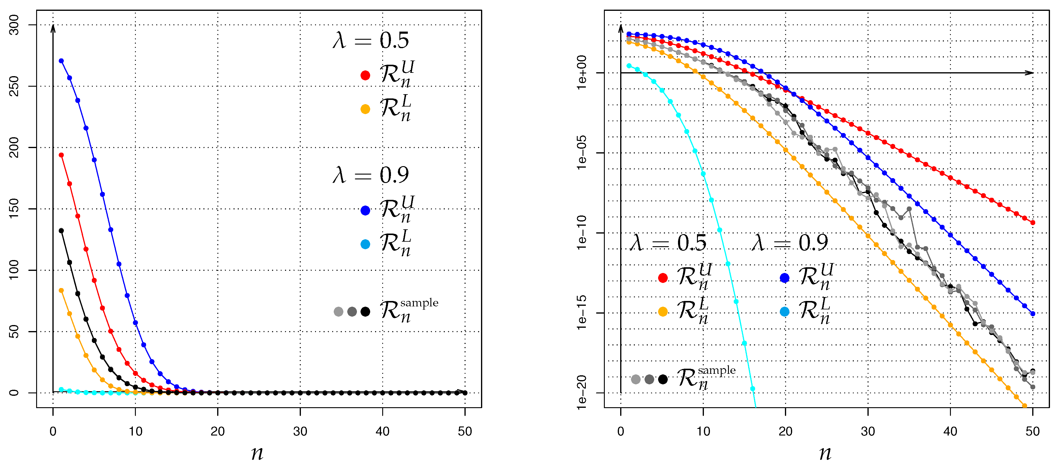
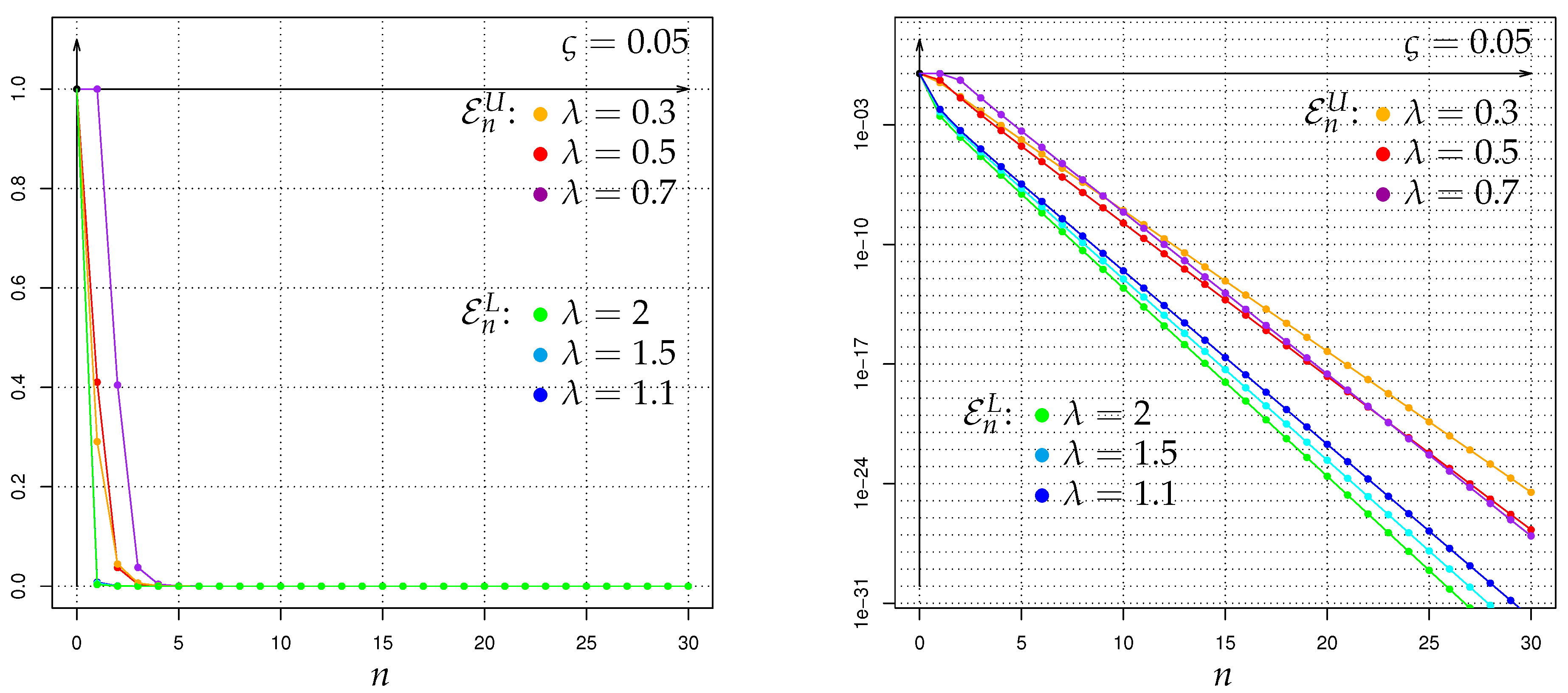
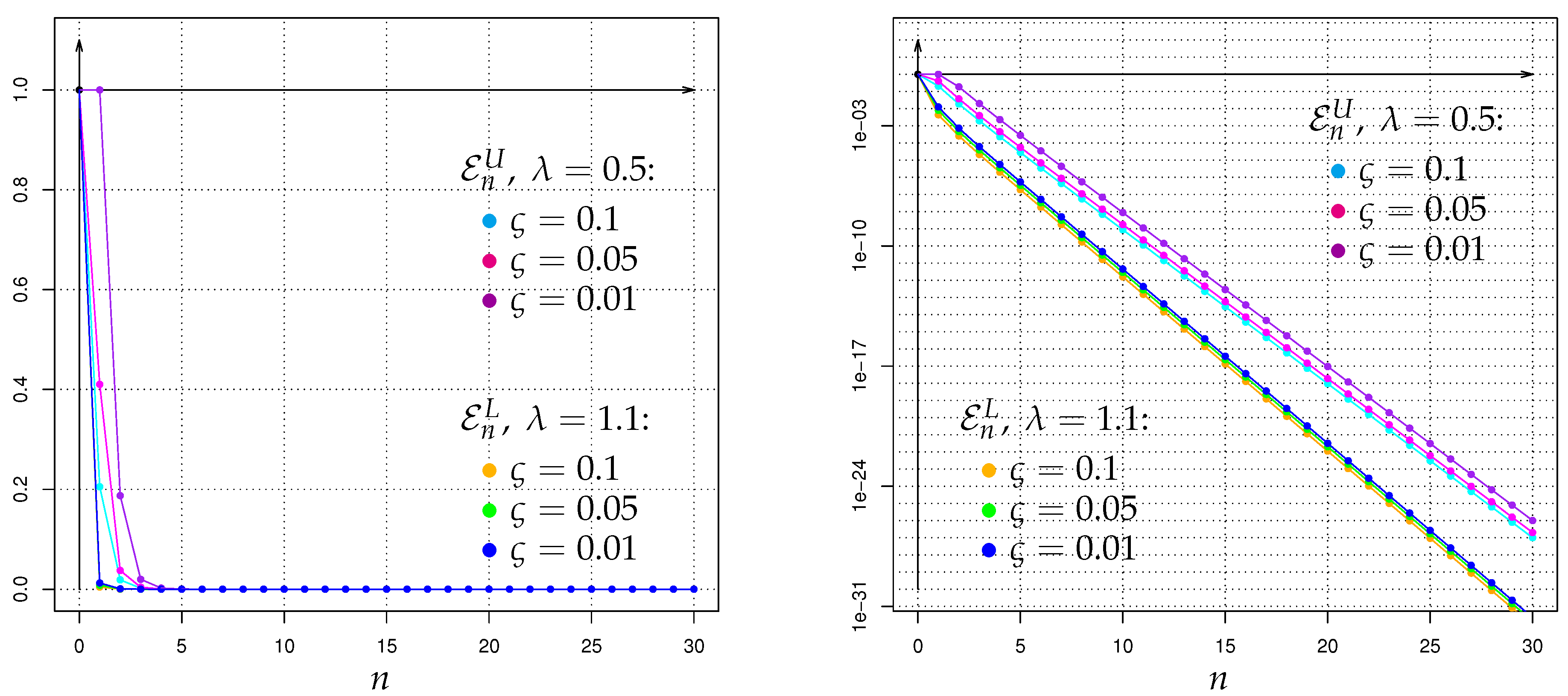
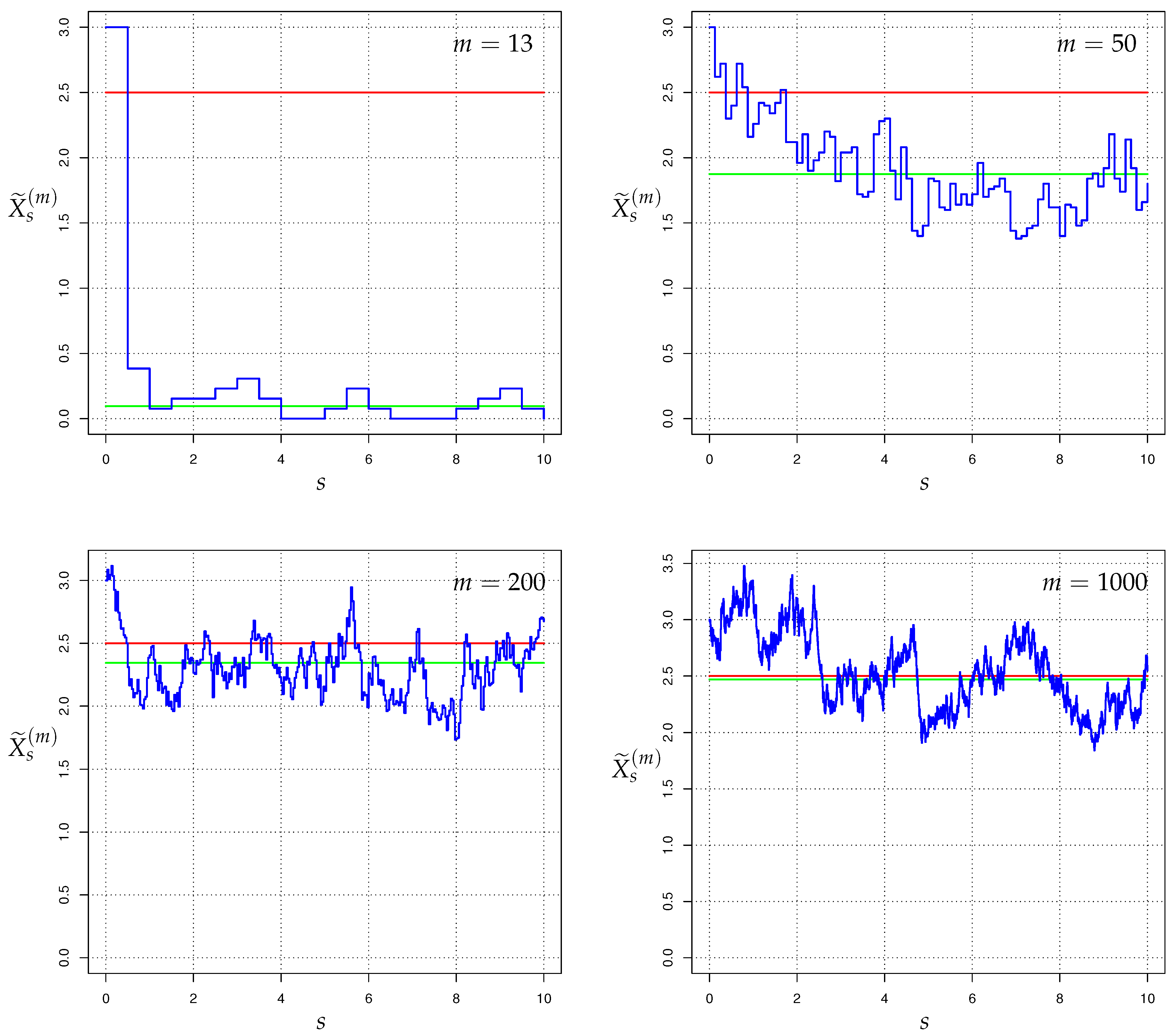


