Spectral-Based SPD Matrix Representation for Signal Detection Using a Deep Neutral Network


Abstract
1. Introduction
2. Spectral Image-Based Signal Detection with a Deep Neural Network
2.1. GoogLeNet
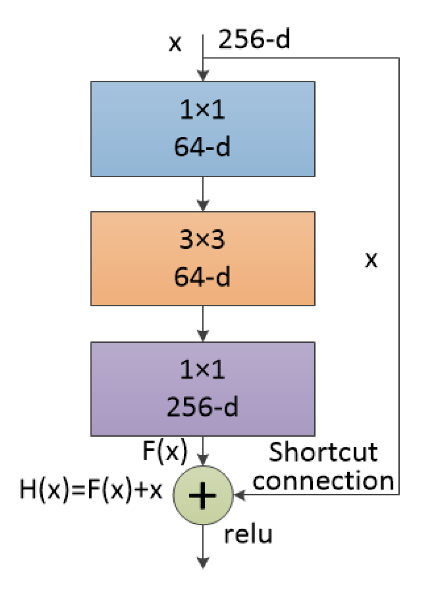
2.2. ResNet
3. Spectral-Based SPD Matrix for Signal Detection with a Deep Neural Network
3.1. Spectral-Based SPD Matrix Construction
3.1.1. SPD Matrix Construction Method Based on Spectrum Transformation
3.1.2. SPD Matrix Construction Method Based on Spectrum Covariance
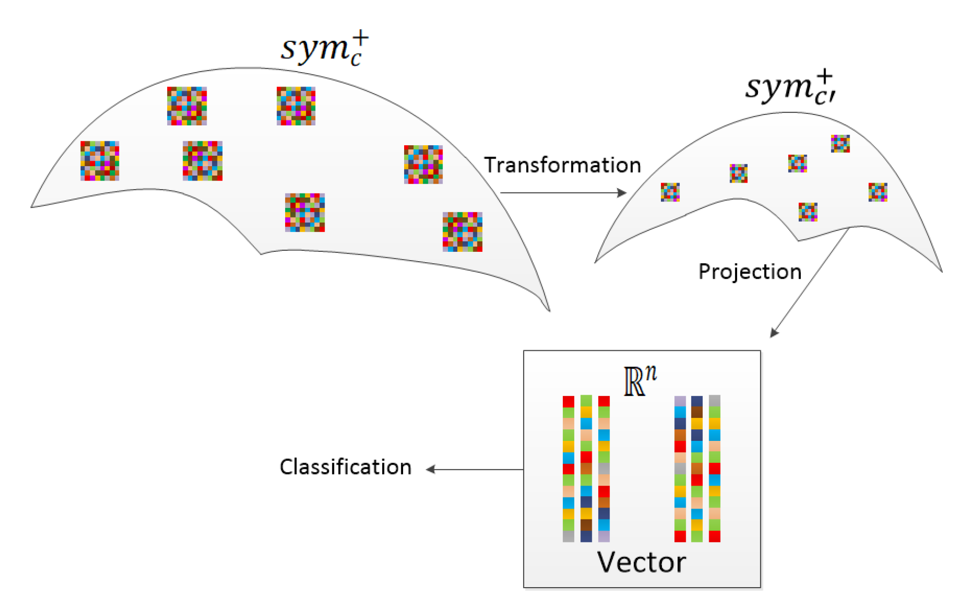
3.2. SPDnet
4. Results
4.1. Experimental Analysis of Simulation Data
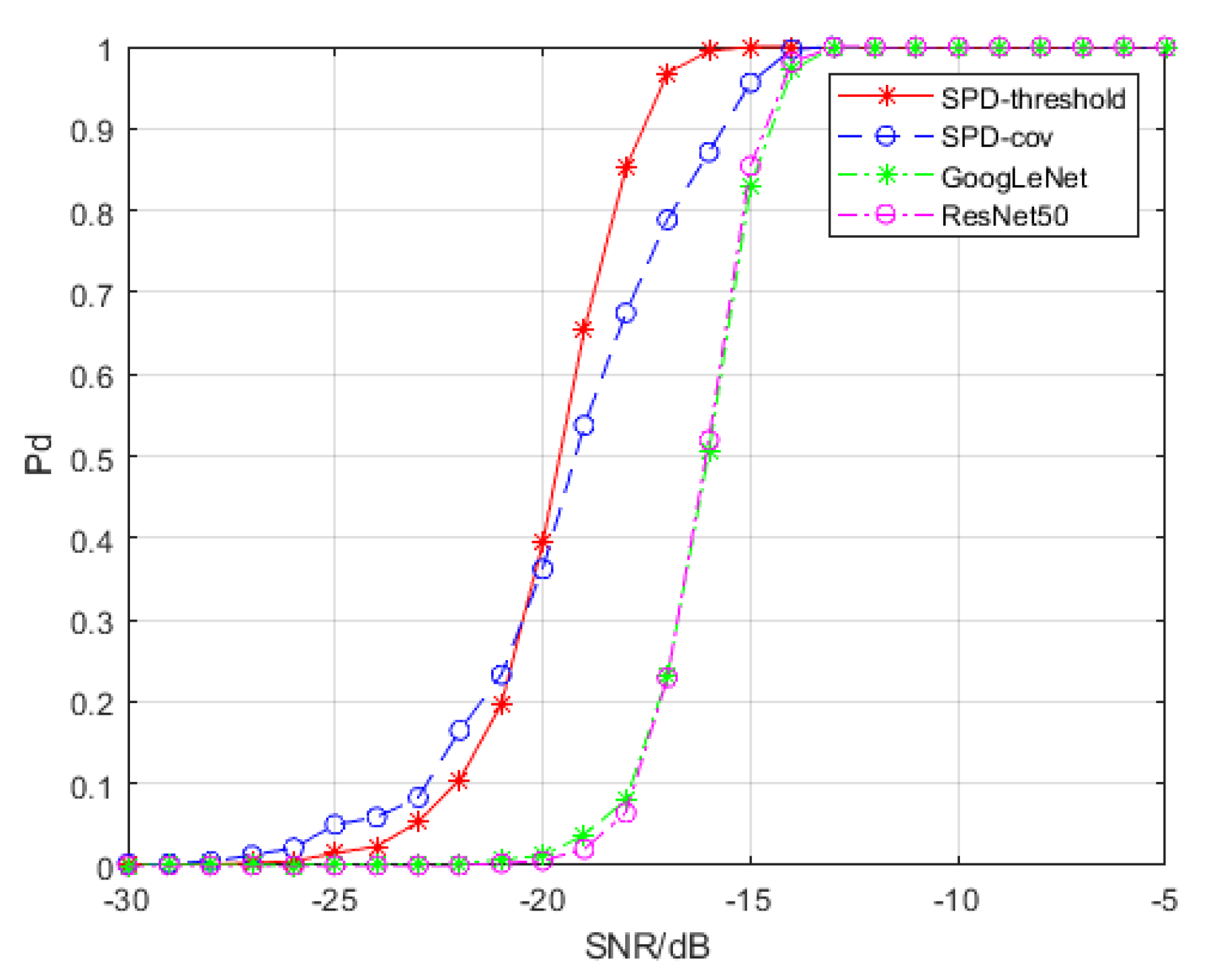
4.1.1. Comparison with Convolutional Neural Networks
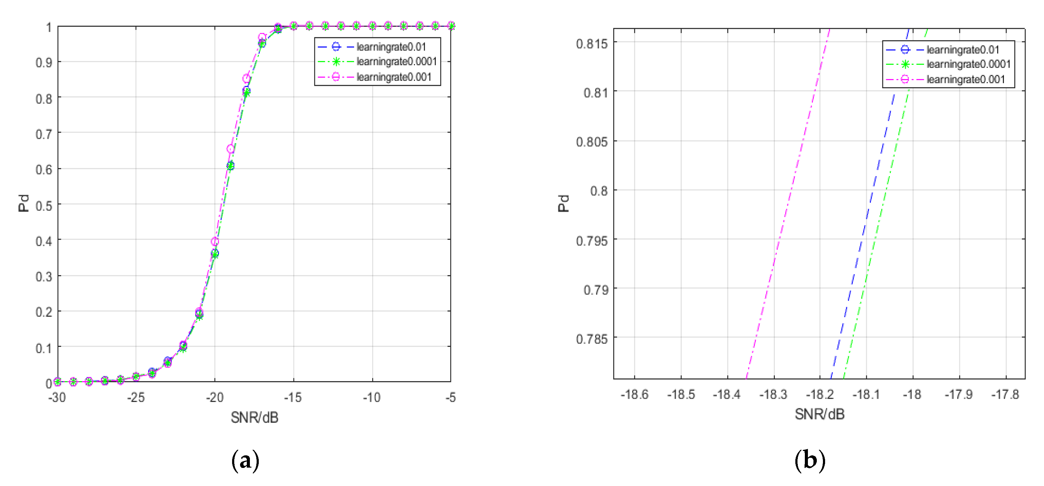
4.1.2. Comparison with Convolutional Neural Networks
4.2. Experimental Analysis of Semi-Physical Simulation Data
5. Conclusions
Author Contributions
Funding
Acknowledgments
Conflicts of Interest
References
- Nandi, A.; Azzouz, E. Algorithms for automatic modulation recognition of communication signals. IEEE Trans. Commun. 1998, 46, 431–436. [Google Scholar] [CrossRef]
- Hsue, S.Z.; Soliman, S.S. Automatic modulation classification using zero crossing. IEEE Proc. 1990, 137, 459–464. [Google Scholar] [CrossRef]
- Hameed, F.; Dobre, O.A.; Popescu, D. On the likelihood-based approach to modulation classification. IEEE Trans. Wirel. Commun. 2009, 8, 5884–5892. [Google Scholar] [CrossRef]
- Reichert, J. Automatic classification of communication signals using higher order statistics. In Proceedings of the IEEE International Conference on Acoustics, Speech, and Signal Processing, Philadelphia, PA, USA, 23–26 March 1992; pp. 221–224. [Google Scholar]
- Pennec, X.; Fillard, P.; Ayache, N. A Riemannian Framework for Tensor Computing. Int. J. Comput. Vis. 2006, 66, 41–66. [Google Scholar] [CrossRef]
- Huang, Z.; Wang, R.; Li, X.; Liu, W.; Shan, S.; Van Gool, L.; Chen, X. Geometry-Aware Similarity Learning on SPD Manifolds for Visual Recognition. IEEE Trans. Circuits Syst. Video Technol. 2018, 28, 2513–2523. [Google Scholar] [CrossRef]
- Harandi, M.; Salzmann, M.; Hartley, R. Dimensionality Reduction on SPD Manifolds: The Emergence of Geometry-Aware Methods. IEEE Trans. Pattern Anal. Mach. Intell. 2018, 40, 48–62. [Google Scholar] [CrossRef] [PubMed]
- Ionescu, C.; Vantzos, O.; Sminchisescu, C. Matrix backpropagation for deep networks with structured layers. In Proceedings of the IEEE International Conference on Computer Vision, Santiago, Chile, 13–16 December 2015; pp. 2965–2973. [Google Scholar]
- Herath, S.; Harandi, M.; Porikli, F. Learning an invariant hilbert space for domain adaptation. In Proceedings of the IEEE Conference on Computer Vision and Pattern Recognition (CVPR), Honolulu, HI, USA, 21–26 July 2017; pp. 3845–3854. [Google Scholar]
- Zhang, J.; Wang, L.; Zhou, L.; Li, W. Exploiting structure sparsity for covariance-based visual representation. arXiv 2016, arXiv:1610.08619. [Google Scholar]
- Zhou, L.; Wang, L.; Zhang, J.; Shi, Y.; Gao, Y. Revisiting metric learning for SPD matrix based visual representation. In Proceedings of the IEEE Conference on Computer Vision and Pattern Recognition (CVPR), Honolulu, HI, USA, 21–26 July 2017; pp. 3241–3249. [Google Scholar]
- Brooks, D.A.; Schwander, O.; Barbaresco, F.; Schneider, J.Y.; Cord, M. Exploring complex time-series representations for Riemannian machine learning of radar data. In Proceedings of the 2019 IEEE International Conference on Acoustics, Speech and Signal Processing, Brighton, UK, 12–17 May 2019; pp. 3672–3676. [Google Scholar]
- Hua, X.; Cheng, Y.; Wang, H.; Qin, Y. Robust Covariance Estimators Based on Information Divergences and Riemannian Manifold. Entropy 2018, 20, 219. [Google Scholar] [CrossRef]
- Hua, X.; Fan, H.; Cheng, Y.; Wang, H.; Qin, Y. Information Geometry for Radar Target Detection with Total Jensen–Bregman Divergence. Entropy 2018, 20, 256. [Google Scholar] [CrossRef]
- Wong, K.; Zhang, J.; Jiang, H. Multi-sensor signal processing on a PSD matrix manifold. In Proceedings of the 2016 IEEE Sensor Array and Multichannel Signal Processing Workshop, Rio de Janeiro, Brazil, 10–13 July 2016; pp. 1–5. [Google Scholar]
- Hua, X.; Shi, Y.; Zeng, Y.; Chen, C.; Lu, W.; Cheng, Y.; Wang, H. A divergence mean-based geometric detector with a pre-processing procedure. Measurement 2019, 131, 640–646. [Google Scholar] [CrossRef]
- Hua, X.; Cheng, Y.; Wang, H.; Qin, Y.; Li, Y. Geometric means and medians with applications to target detection. IET Signal Process. 2017, 11, 711–720. [Google Scholar] [CrossRef]
- Fathy, M.E.; Alavi, A.; Chellappa, R. Discriminative Log-Euclidean Feature Learning for Sparse Representation-Based Recognition of Faces from Videos. In Proceedings of the International Joint Conferences on Artificial Intelligence, IJCAI, New York, NY, USA, 9–15 July 2016; pp. 3359–3367. [Google Scholar]
- Zhang, S.; Kasiviswanathan, S.; Yuen, P.C.; Harandi, M. Online dictionary learning on symmetric positive definite manifolds with vision applications. In Proceedings of the Twenty-Ninth AAAI Conference on Artificial Intelligence, AAAI, Austin, TX, USA, 25–30 January 2015. [Google Scholar]
- Huang, Z.; Van Gool, L. A Riemannian Network for SPD Matrix Learning. In Proceedings of the Thirty-First AAAI Conference on Artificial Intelligence, AAAI, San Francisco, CA, USA, 4–9 February 2017. [Google Scholar]
- Dong, Z.; Jia, S.; Zhang, C.; Pei, M.; Wu, Y. Deep manifold learning of symmetric positive definite matrices with application to face recognition. In Proceedings of the Thirty-First AAAI Conference on Artificial Intelligence, AAAI, San Francisco, CA, USA, 4–9 February 2017. [Google Scholar]
- Zhang, T.; Zheng, W.; Cui, Z.; Zong, Y.; Li, C.; Zhou, X.; Yang, J. Deep Manifold-to-Manifold Transforming Network for Skeleton-based Action Recognition. IEEE Trans. Multimed. 2020, 1. [Google Scholar] [CrossRef]
- Gao, Z.; Wu, Y.; Bu, X.; Yu, T.; Yuan, J.; Jia, Y. Learning a robust representation via a deep network on symmetric positive definite manifolds. Pattern Recognit. 2019, 92, 1–12. [Google Scholar] [CrossRef]
- Bronstein, M.M.; Bruna, J.; LeCun, Y.; Szlam, A.; VanderGheynst, P. Geometric Deep Learning: Going beyond Euclidean data. IEEE Signal Process. Mag. 2017, 34, 18–42. [Google Scholar] [CrossRef]
- Krizhevsky, A.; Sutskever, I.; Hinton, G.E. Pdf ImageNet classification with deep convolutional neural networks. Commun. ACM 2017, 60, 84–90. [Google Scholar] [CrossRef]
- Szegedy, C.; Liu, W.; Jia, Y.; Sermanet, P.; Reed, S.; Anguelov, D.; Erhan, D.; Vanhoucke, V.; Rabinovich, A. Going deeper with convolutions. In Proceedings of the IEEE Conference on Computer Vision and Pattern Recognition, IEEE, Boston, MA, USA, 8–12 June 2015; pp. 1–9. [Google Scholar]
- He, K.; Zhang, X.; Ren, S.; Sun, J. Deep residual learning for image recognition. In Proceedings of the IEEE Conference on Computer Vision and Pattern Recognition, Las Vegas, NV, USA, 26 June–1 July 2016; pp. 770–778. [Google Scholar]
- Wang, R.; Guo, H.; Davis, L.S.; Dai, Q. Covariance discriminative learning: A natural and efficient approach to image set classification. In Proceedings of the 2012 IEEE Conference on Computer Vision and Pattern Recognition, Providence, RI, USA, 18–20 June 2012; pp. 2496–2503. [Google Scholar]
- The McMaster IPIX Radar Sea Clutter Database. Available online: http://soma.ece.mcmaster.ca/ipix/ (accessed on 20 April 2020).


| Model | Spectral Transformation SPD Matrix Network | Spectral Covariance SPD Matrix Network | GoogLeNet with Time-Frequency Spectra | ResNet50 with Time-Frequency Spectra | |
|---|---|---|---|---|---|
| SCR(dB) | |||||
| −5 | Less than 0.01 | Less than 0.01 | Less than 0.01 | Less than 0.01 | |
| −10 | Less than 0.01 | Less than 0.01 | Less than 0.01 | Less than 0.01 | |
| −15 | Less than 0.01 | 0.23 | 1.12 | 0.50 | |
| −20 | 2.47 | 2.22 | 32.97 | 25.95 | |
| −25 | 18.80 | 16.65 | 99.96 | 39.01 | |
| −30 | 29.80 | 14.00 | 99.98 | 49.15 | |
| Model | Spectral Transformation SPD Matrix Network | Spectral Covariance SPD Matrix Network | GoogLeNet with Time-Frequency Spectra | ResNet50 with Time-Frequency Spectra |
|---|---|---|---|---|
| Total Training Time(Min) | 67.6 | 69.5 | 2068.0 | 7083.3 |
| Total Number of Epochs | 500 | 500 | 2000 | 2000 |
| The Average Time per 100 Epochs(Min) | 13.5 | 13.9 | 103.4 | 354.2 |
| Model | Learning Rate 0.01 | Learning Rate 0.001 | Learning Rate 0.0001 | |
|---|---|---|---|---|
| SCR(dB) | ||||
| −5 | Less than 0.01 | Less than 0.01 | Less than 0.01 | |
| −10 | Less than 0.01 | Less than 0.01 | Less than 0.01 | |
| −15 | Less than 0.01 | Less than 0.01 | Less than 0.01 | |
| −20 | 8.02 | 2.50 | 12.42 | |
| −25 | 15.51 | 19.44 | 33.00 | |
| −30 | 26.38 | 29.98 | 37.00 | |
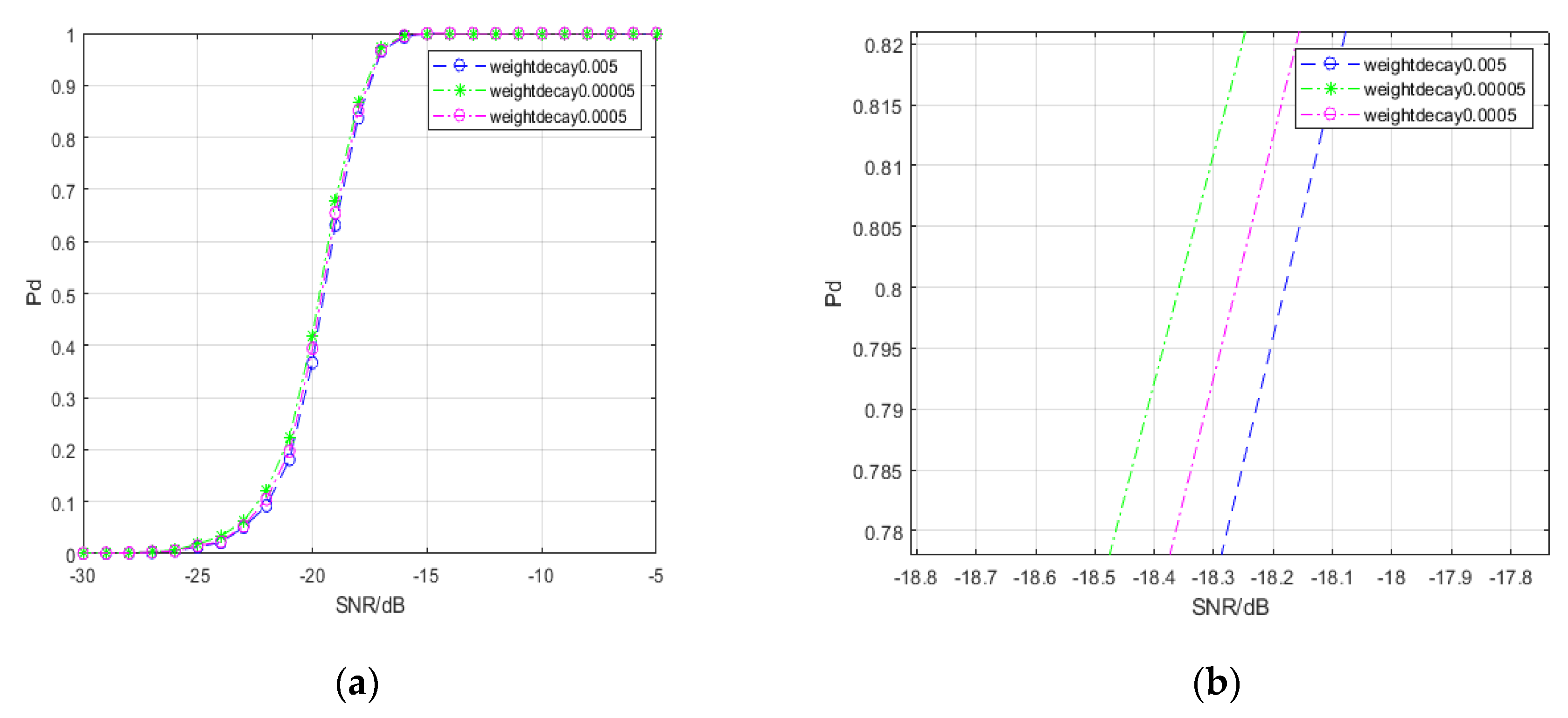
| Model | Weight Decay 0.005 | Weight Decay 0.0005 | Weight Decay 0.00005 | |
|---|---|---|---|---|
| SCR(dB) | ||||
| −5 | Less than 0.01 | Less than 0.01 | Less than 0.01 | |
| −10 | Less than 0.01 | Less than 0.01 | Less than 0.01 | |
| −15 | Less than 0.01 | Less than 0.01 | Less than 0.01 | |
| −20 | 9.94 | 2.50 | 9.93 | |
| −25 | 23.36 | 19.40 | 23.5 | |
| −30 | 27.28 | 29.98 | 27.28 | |
| Model | 6 Layers | 8 Layers | 10 Layers | |
|---|---|---|---|---|
| SCR(dB) | ||||
| −5 | Less than 0.01 | Less than 0.01 | Less than 0.01 | |
| −10 | Less than 0.01 | Less than 0.01 | Less than 0.01 | |
| −15 | 0.08 | Less than 0.01 | Less than 0.01 | |
| −20 | 4.82 | 2.51 | 6.13 | |
| −25 | 26.33 | 19.44 | 24.08 | |
| −30 | 28.10 | 30.10 | 28.42 | |
| Number | Name |
|---|---|
| 1 | 19980223_171533_ANTSTEP |
| 2 | 19980223_171811_ANTSTEP |
| 3 | 19980223_172059_ANTSTEP |
| 4 | 19980223_172410_ANTSTEP |
| 5 | 19980223_172650_ANTSTEP |
| 6 | 19980223_184853_ANTSTEP |
| 7 | 19980223_185157_ANTSTEP |
| Pulse Repetition Frequency | Carrier Frequency | The Length of the Pulse | Range Resolution | Polarization Mode |
|---|---|---|---|---|
| 1000 Hz | 9.39 GHz | 60,000 | 3 m | HH |
| Model | Spectral Transformation SPD Matrix Network | Spectral Covariance SPD Matrix Network | GoogLeNet with Time-Frequency Spectra | ResNet50 with Time-Frequency Spectra | |
|---|---|---|---|---|---|
| SCR(dB) | |||||
| −5 | Less than 0.01 | 0.25 | Less than 0.01 | Less than 0.01 | |
| −10 | Less than 0.01 | 0.42 | Less than 0.01 | Less than 0.01 | |
| −15 | 0.08 | 2.17 | 0.15 | Less than 0.01 | |
| −20 | 6.90 | 13.92 | 14.49 | 10.52 | |
© 2020 by the authors. Licensee MDPI, Basel, Switzerland. This article is an open access article distributed under the terms and conditions of the Creative Commons Attribution (CC BY) license (http://creativecommons.org/licenses/by/4.0/).
Share and Cite
Wang, J.; Hua, X.; Zeng, X. Spectral-Based SPD Matrix Representation for Signal Detection Using a Deep Neutral Network. Entropy 2020, 22, 585. https://doi.org/10.3390/e22050585
Wang J, Hua X, Zeng X. Spectral-Based SPD Matrix Representation for Signal Detection Using a Deep Neutral Network. Entropy. 2020; 22(5):585. https://doi.org/10.3390/e22050585
Chicago/Turabian StyleWang, Jiangyi, Xiaoqiang Hua, and Xinwu Zeng. 2020. "Spectral-Based SPD Matrix Representation for Signal Detection Using a Deep Neutral Network" Entropy 22, no. 5: 585. https://doi.org/10.3390/e22050585
APA StyleWang, J., Hua, X., & Zeng, X. (2020). Spectral-Based SPD Matrix Representation for Signal Detection Using a Deep Neutral Network. Entropy, 22(5), 585. https://doi.org/10.3390/e22050585