On Geometry of Information Flow for Causal Inference


Abstract
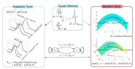
1. Introduction
- In traditional methods, causality is estimated by probabilistic terms. In this study, we present analytical and data driven approach to identify causality by geometric methods, and thus also a unifying perspective.
- We show that a derivative (if it exists) of the underlining function of the time series has a close relationship to the transfer entropy (Section 2.3).
- We provide a new tool called to identify the causality by geometric terms (Section 3).
- Correlation dimension can be used as a measurement for dynamics of a dynamical system. We will show that this measurement can be used to identify the causality (Section 3).
2. The Problem Setup
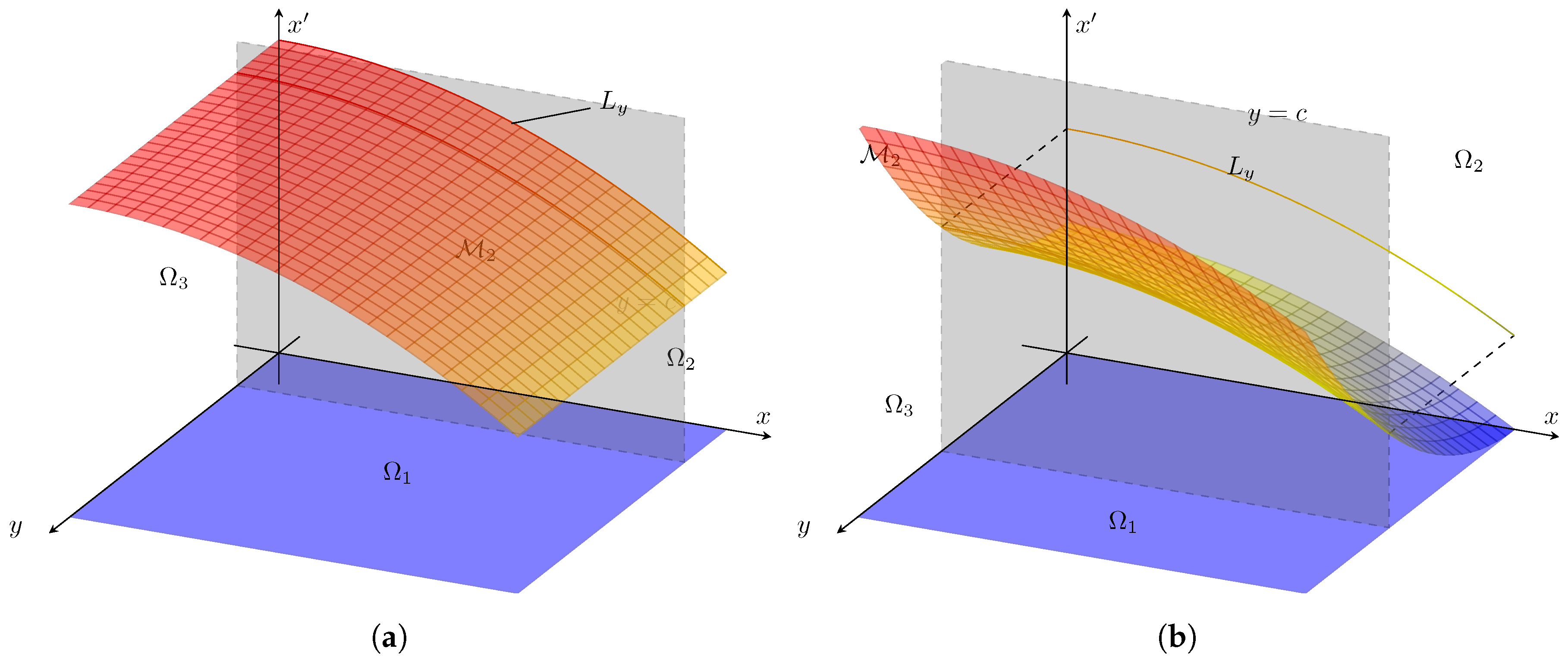
2.1. In Geometric Terms
- If for all , then for all .
- If for some , then for some , and then is not a sufficient description of what should really be written . We have assumed throughout.
2.2. In Probabilistic Terms
Relative Entropy for a Function of Random Variables
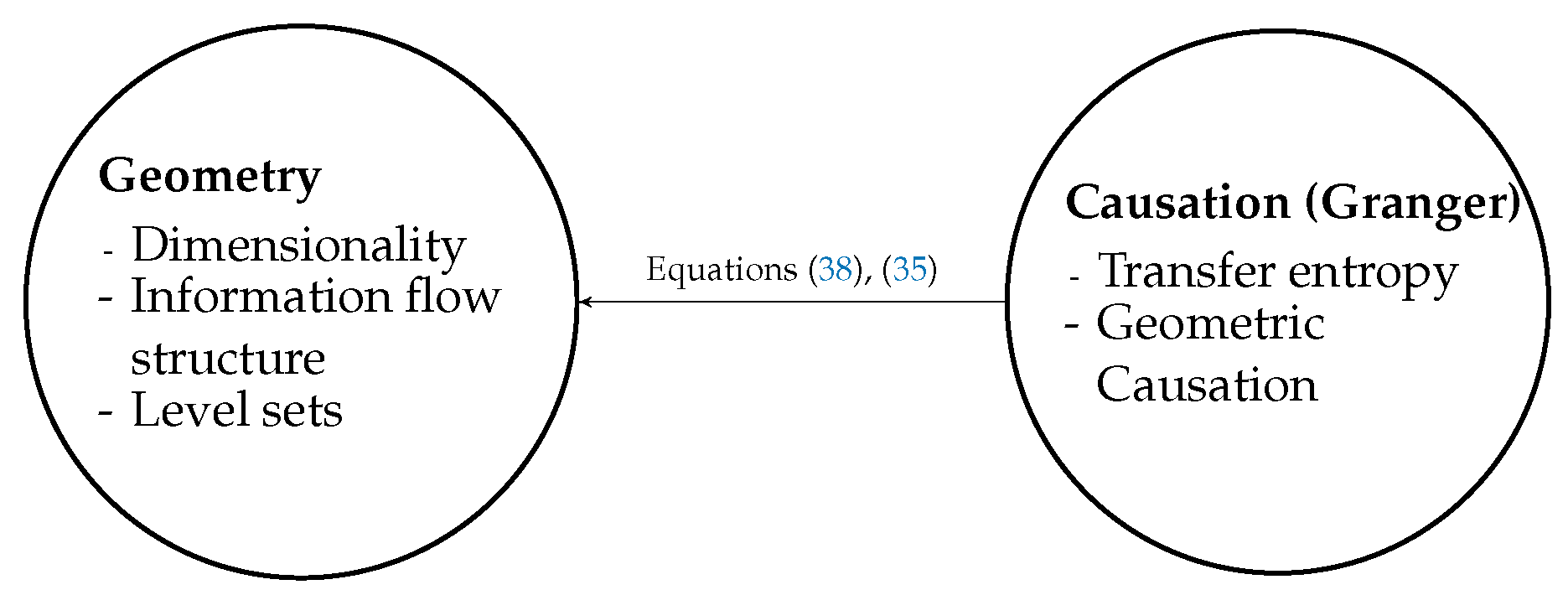
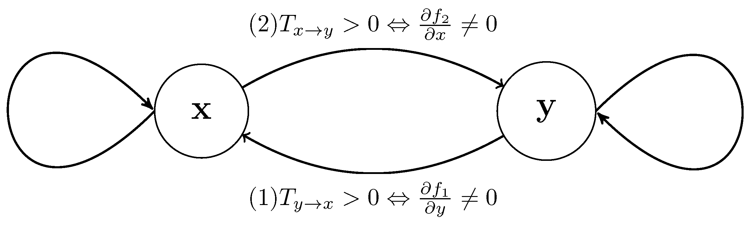
2.3. Relating Transfer Entropy to a Geometric Bound
3. Geometry of Information Flow
3.1. Relating the Information Flow as Geometric Orientation of Data
3.2. Measure Causality by Correlation Dimension
4. Results and Discussion
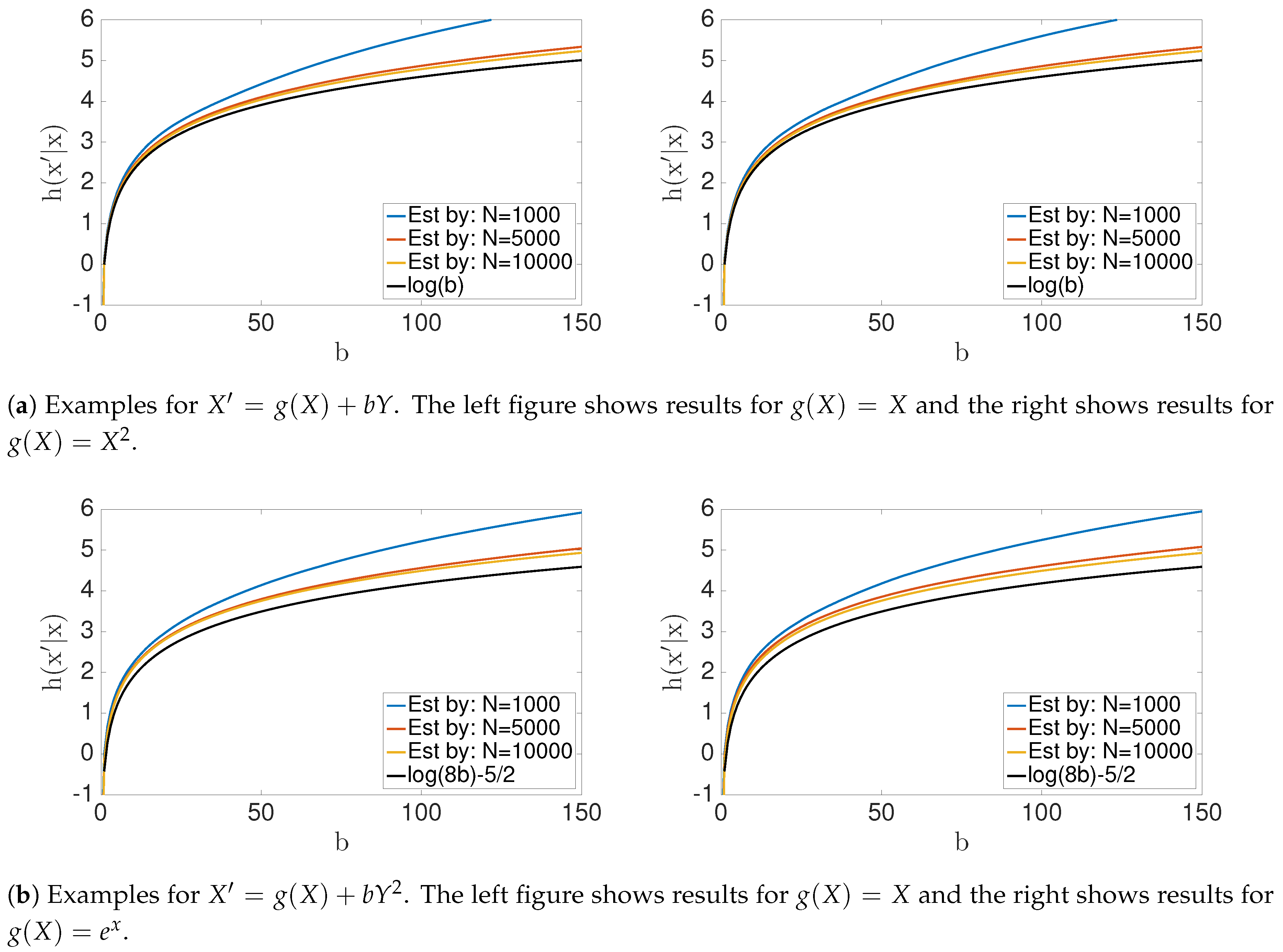
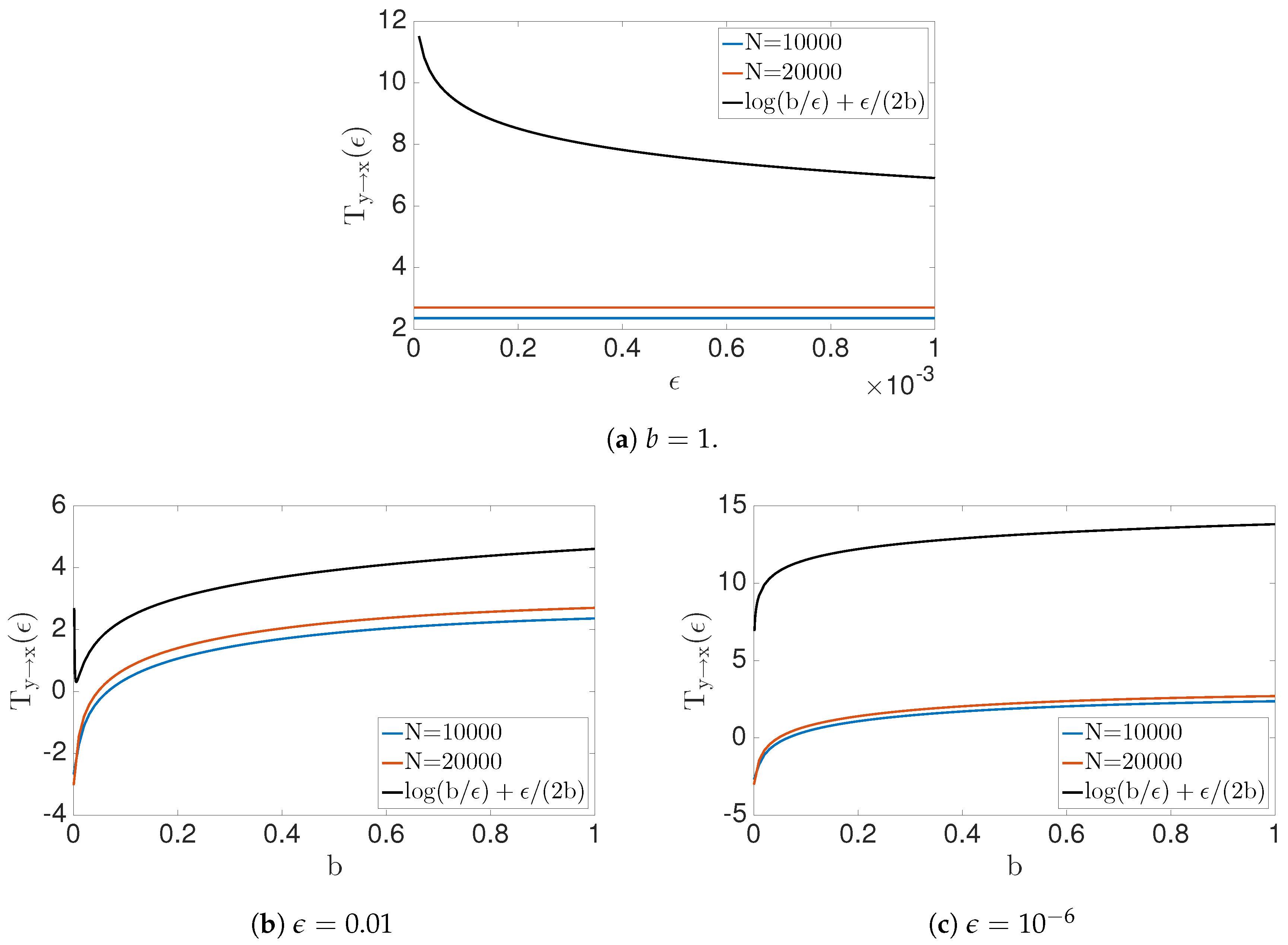
4.1. Transfer Entropy
4.2. Geometric Information Flow
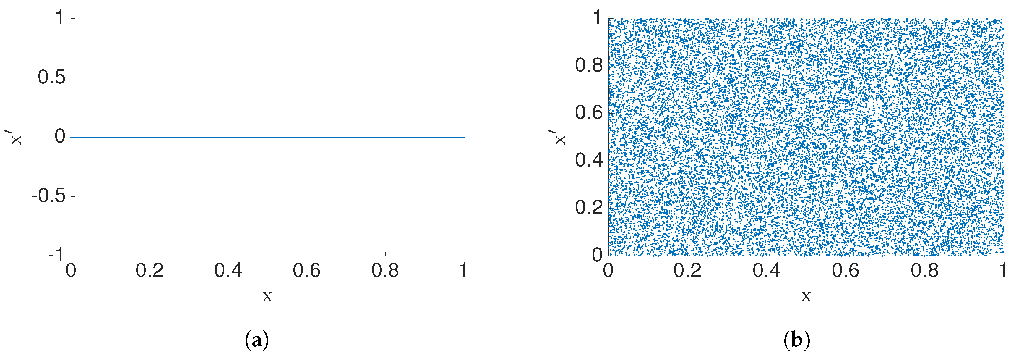
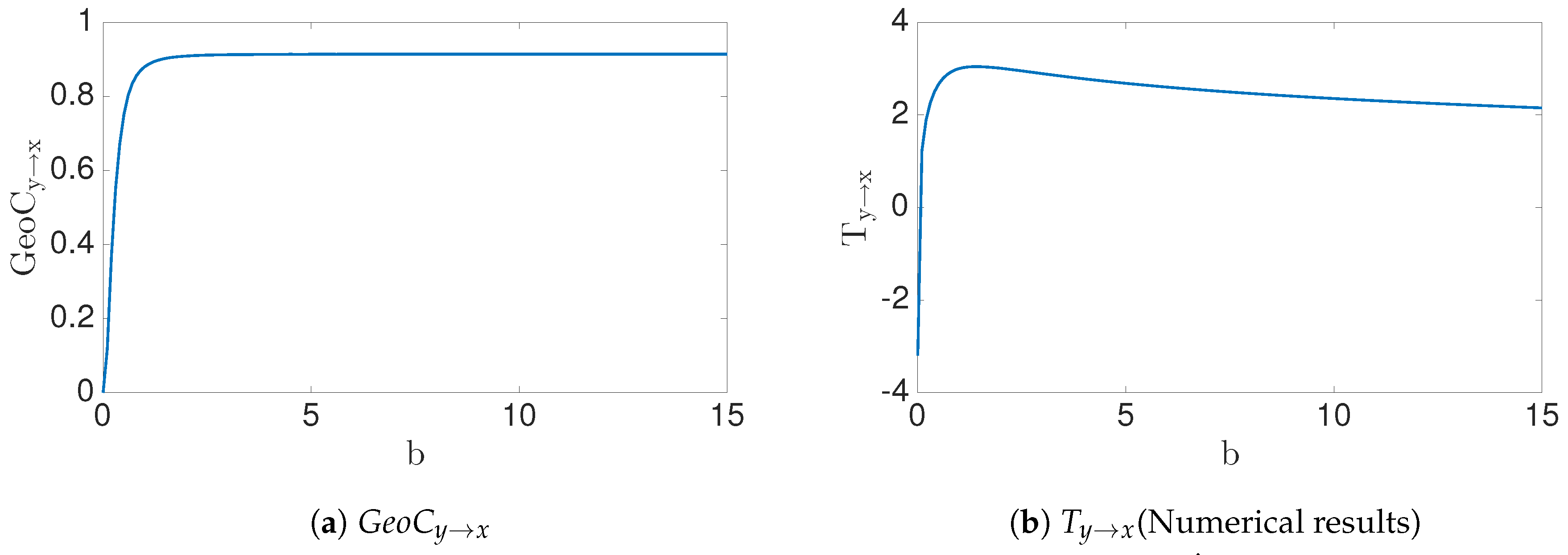
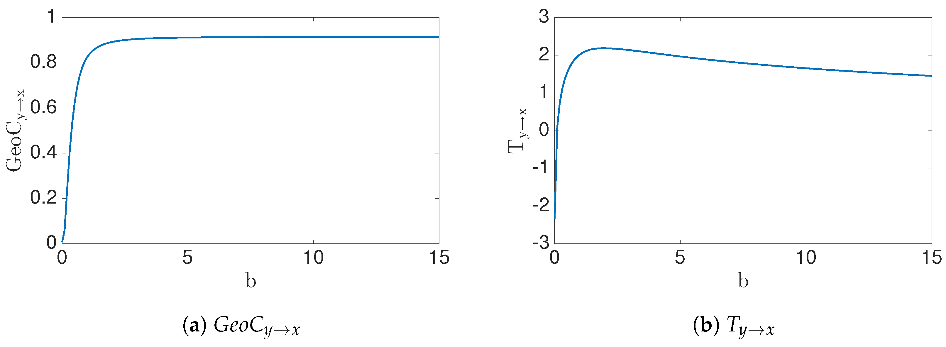
4.3. Synthetic Data: with
4.4. Synthetic Data: Nonlinear Cases
4.5. Application Data
5. Conclusions
Author Contributions
Funding
Acknowledgments
Conflicts of Interest
Appendix A. On the Asymmetric Spaces Transfer Operators
References
- Williams, C.J.F. “Aristotle’s Physics, Books I and II”, Translated with Introduction and Notes by W. Charlton. Mind 1973, 82, 617. [Google Scholar] [CrossRef]
- Falcon, A. Aristotle on Causality. In The Stanford Encyclopedia of Philosophy, Spring 2019 ed.; Zalta, E.N., Ed.; Metaphysics Research Lab, Stanford University: Stanford, CA, USA, 2019. [Google Scholar]
- Russell, B. I.—On the Notion of Cause. Proc. Aristot. Soc. 1913, 13, 1–26. [Google Scholar] [CrossRef]
- Bollt, E.M. Open or closed? Information flow decided by transfer operators and forecastability quality metric. Chaos Interdiscip. J. Nonlinear Sci. 2018, 28, 075309. [Google Scholar] [CrossRef] [PubMed]
- Hendry, D.F. The Nobel Memorial Prize for Clive W. J. Granger. Scand. J. Econ. 2004, 106, 187–213. [Google Scholar] [CrossRef]
- Wiener, N. The theory of prediction. In Mathematics for the Engineer; McGraw-Hill: New York, NY, USA, 1956. [Google Scholar]
- Schreiber, T. Measuring Information Transfer. Phys. Rev. Lett. 2000, 85, 461–464. [Google Scholar] [CrossRef] [PubMed]
- Bollt, E.; Santitissadeekorn, N. Applied and Computational Measurable Dynamics; Society for Industrial and Applied Mathematics: Philadelphia, PA, USA, 2013. [Google Scholar] [CrossRef]
- Barnett, L.; Barrett, A.B.; Seth, A.K. Granger Causality and Transfer Entropy Are Equivalent for Gaussian Variables. Phys. Rev. Lett. 2009, 103, 238701. [Google Scholar] [CrossRef]
- Sugihara, G.; May, R.; Ye, H.; Hsieh, C.h.; Deyle, E.; Fogarty, M.; Munch, S. Detecting Causality in Complex Ecosystems. Science 2012, 338, 496–500. [Google Scholar] [CrossRef] [PubMed]
- Sun, J.; Bollt, E.M. Causation entropy identifies indirect influences, dominance of neighbors and anticipatory couplings. Phys. D Nonlinear Phenom. 2014, 267, 49–57. [Google Scholar] [CrossRef]
- Sun, J.; Taylor, D.; Bollt, E. Causal Network Inference by Optimal Causation Entropy. SIAM J. Appl. Dyn. Syst. 2015, 14, 73–106. [Google Scholar] [CrossRef]
- Bollt, E.M.; Sun, J.; Runge, J. Introduction to Focus Issue: Causation inference and information flow in dynamical systems: Theory and applications. Chaos Interdiscip. J. Nonlinear Sci. 2018, 28, 075201. [Google Scholar] [CrossRef]
- Runge, J.; Bathiany, S.; Bollt, E.; Camps-Valls, G.; Coumou, D.; Deyle, E.; Glymour, C.; Kretschmer, M.; Mahecha, M.D.; Muñoz-Marí, J.; et al. Inferring causation from time series in Earth system sciences. Nat. Commun. 2019, 10, 1–13. [Google Scholar] [CrossRef] [PubMed]
- Lord, W.M.; Sun, J.; Ouellette, N.T.; Bollt, E.M. Inference of causal information flow in collective animal behavior. IEEE Trans. Mol. Biol. Multi-Scale Commun. 2016, 2, 107–116. [Google Scholar] [CrossRef]
- Kim, P.; Rogers, J.; Sun, J.; Bollt, E. Causation entropy identifies sparsity structure for parameter estimation of dynamic systems. J. Comput. Nonlinear Dyn. 2017, 12, 011008. [Google Scholar] [CrossRef]
- AlMomani, A.A.R.; Sun, J.; Bollt, E. How Entropic Regression Beats the Outliers Problem in Nonlinear System Identification. arXiv 2019, arXiv:1905.08061. [Google Scholar] [CrossRef] [PubMed]
- Sudu Ambegedara, A.; Sun, J.; Janoyan, K.; Bollt, E. Information-theoretical noninvasive damage detection in bridge structures. Chaos Interdiscip. J. Nonlinear Sci. 2016, 26, 116312. [Google Scholar] [CrossRef]
- Hall, N. Two Concepts of Causation. In Causation and Counterfactuals; Collins, J., Hall, N., Paul, L., Eds.; MIT Press: Cambridge, MA, USA, 2004; pp. 225–276. [Google Scholar]
- Pearl, J. Bayesianism and Causality, or, Why I Am Only a Half-Bayesian. In Foundations of Bayesianism; Corfield, D., Williamson, J., Eds.; Kluwer Academic Publishers: Dordrecht, The Netherlands, 2001; pp. 19–36. [Google Scholar]
- White, H.; Chalak, K.; Lu, X. Linking Granger Causality and the Pearl Causal Model with Settable Systems. JMRL Workshop Conf. Proc. 2011, 12, 1–29. [Google Scholar]
- White, H.; Chalak, K. Settable Systems: An Extension of Pearl’s Causal Model with Optimization, Equilibrium, and Learning. J. Mach. Learn. Res. 2009, 10, 1759–1799. [Google Scholar]
- Bollt, E. Synchronization as a process of sharing and transferring information. Int. J. Bifurc. Chaos 2012, 22. [Google Scholar] [CrossRef]
- Lasota, A.; Mackey, M. Chaos, Fractals, and Noise: Stochastic Aspects of Dynamics; Springer: New York, NY, USA, 2013. [Google Scholar]
- Pinsker, M.S. Information and information stability of random variables and processes. Dokl. Akad. Nauk SSSR 1960, 133, 28–30. [Google Scholar]
- Boucheron, S.; Lugosi, G.; Massart, P. Concentration Inequalities: A Nonasymptotic Theory of Independence; Oxford University Press: Oxford, UK, 2013. [Google Scholar]
- Sauer, T.; Yorke, J.A.; Casdagli, M. Embedology. Stat. Phys. 1991, 65, 579–616. [Google Scholar] [CrossRef]
- Sauer, T.; Yorke, J.A. Are the dimensions of a set and its image equal under typical smooth functions? Ergod. Theory Dyn. Syst. 1997, 17, 941–956. [Google Scholar] [CrossRef]
- Grassberger, P.; Procaccia, I. Measuring the strangeness of strange attractors. Phys. D Nonlinear Phenom. 1983, 9, 189–208. [Google Scholar] [CrossRef]
- Grassberger, P.; Procaccia, I. Characterization of Strange Attractors. Phys. Rev. Lett. 1983, 50, 346–349. [Google Scholar] [CrossRef]
- Grassberger, P. Generalized dimensions of strange attractors. Phys. Lett. A 1983, 97, 227–230. [Google Scholar] [CrossRef]
- Kraskov, A.; Stögbauer, H.; Grassberger, P. Estimating mutual information. Phys. Rev. E 2004, 69, 066138. [Google Scholar] [CrossRef]
- Rigney, D.; Goldberger, A.; Ocasio, W.; Ichimaru, Y.; Moody, G.; Mark, R. Multi-channel physiological data: Description and analysis. In Time Series Prediction: Forecasting the Future and Understanding the Past; Addison-Wesley: Boston, MA, USA, 1993; pp. 105–129. [Google Scholar]
- Ichimaru, Y.; Moody, G. Development of the polysomnographic database on CD-ROM. Psychiatry Clin. Neurosci. 1999, 53, 175–177. [Google Scholar] [CrossRef] [PubMed]


| Data | Transfer Entropy (Section 4.1) | Geometric Approach |
|---|---|---|
| Synthetic: f(x,y)=, | Theoretical issues can be noticed. Numerical estimation have boundedness issues when . | Successfully identify the causation for all the cases (). |
| Synthetic: f(x,y)=, | Theoretical issues can be noticed. Numerical estimation have boundedness issues when . | Successfully identify the causation for all the cases (). |
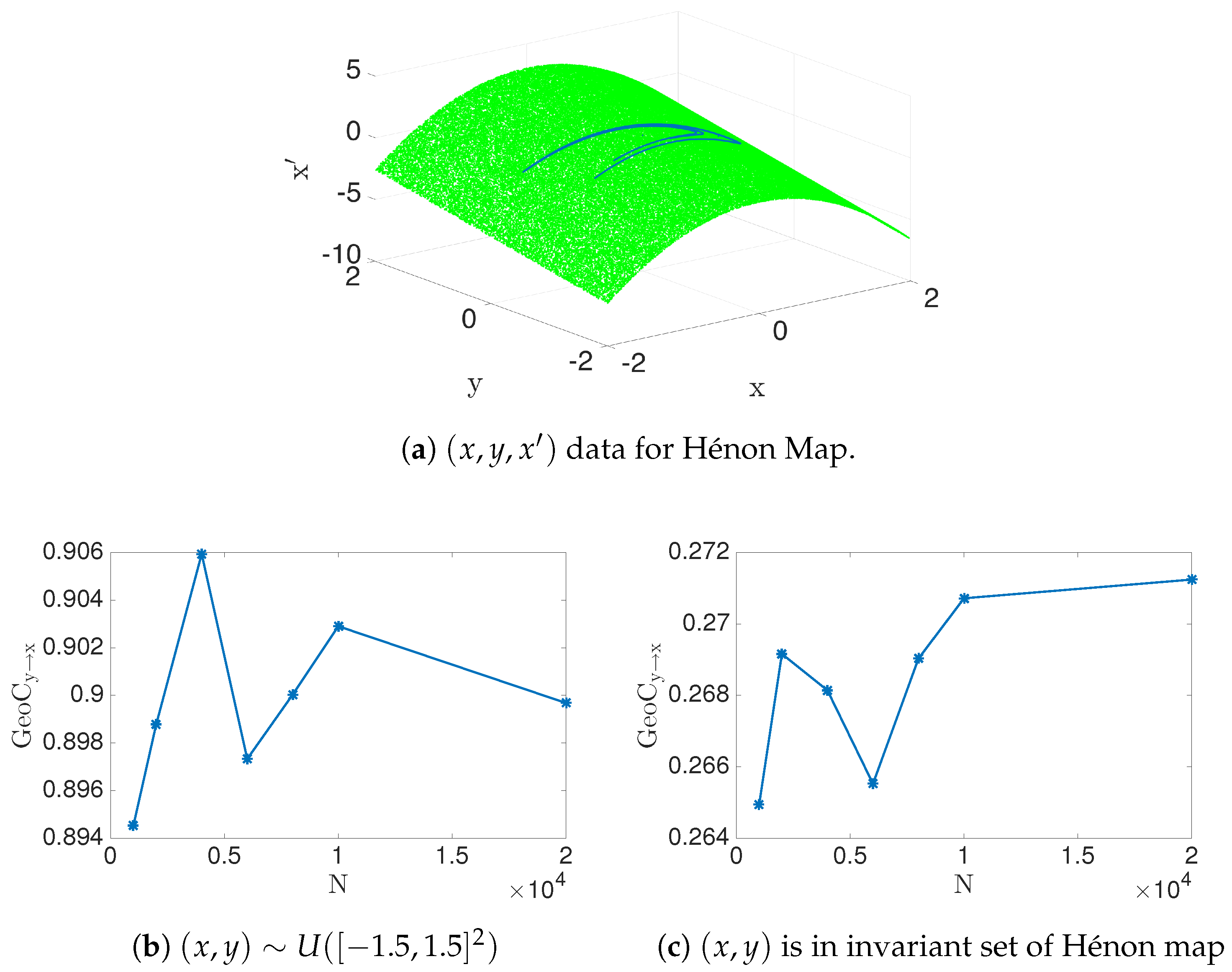
| Hénon map: use data set invariant under the map. | special case of with . Estimated transfer entropy is positive. | Successfully identify the causation. |
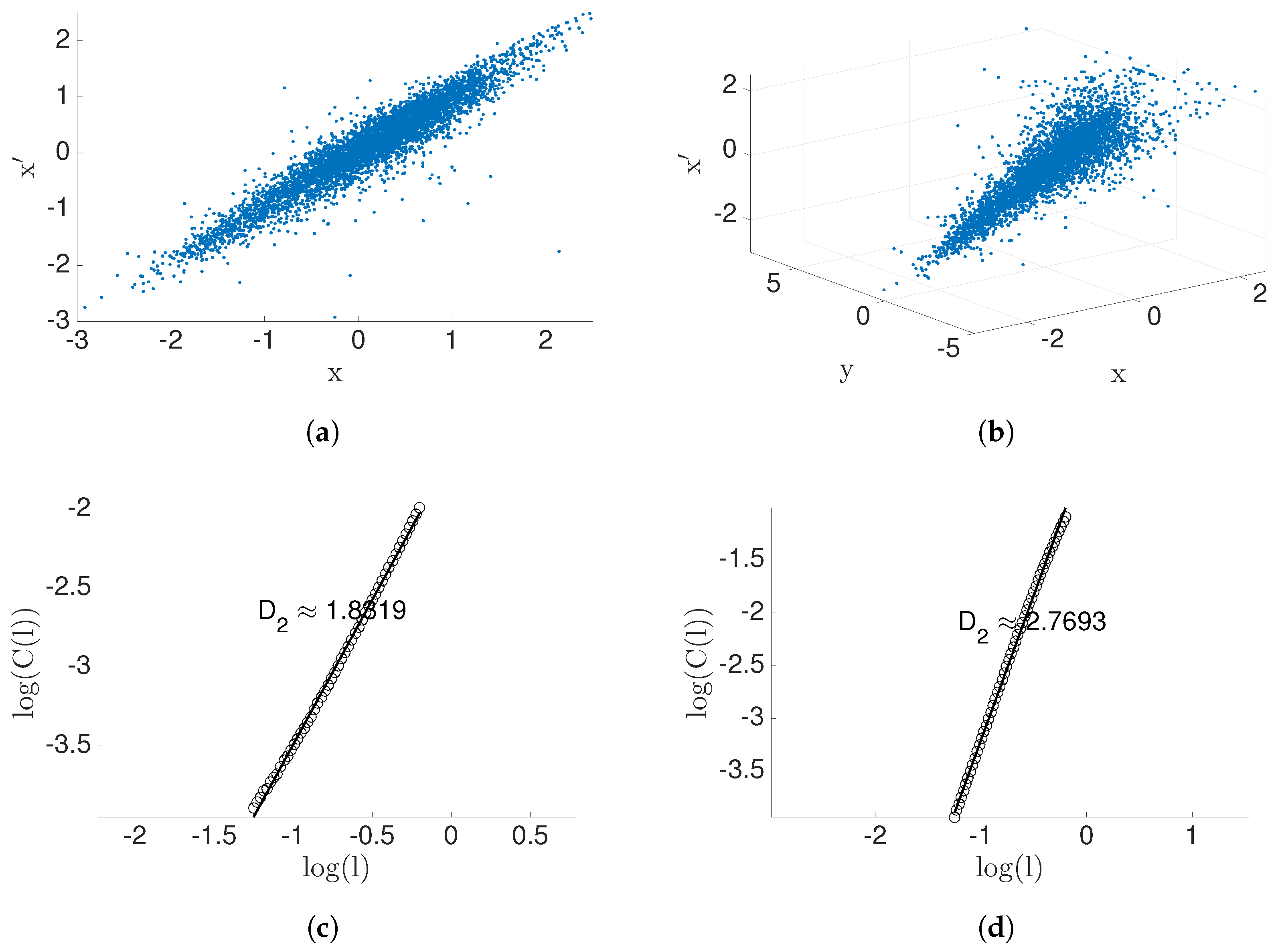
| Application: heart rate vs. breathing rate | Positive transfer entropy. | Identify positive causation. It also provides more details about the data. |
| Domain | ||
|---|---|---|
| 0.90 | 2.4116 | |
| Invariant Set | 0.2712 | 0.7942 |
| 0.0427 | 0.0485 |
© 2020 by the authors. Licensee MDPI, Basel, Switzerland. This article is an open access article distributed under the terms and conditions of the Creative Commons Attribution (CC BY) license (http://creativecommons.org/licenses/by/4.0/).
Share and Cite
Surasinghe, S.; Bollt, E.M. On Geometry of Information Flow for Causal Inference. Entropy 2020, 22, 396. https://doi.org/10.3390/e22040396
Surasinghe S, Bollt EM. On Geometry of Information Flow for Causal Inference. Entropy. 2020; 22(4):396. https://doi.org/10.3390/e22040396
Chicago/Turabian StyleSurasinghe, Sudam, and Erik M. Bollt. 2020. "On Geometry of Information Flow for Causal Inference" Entropy 22, no. 4: 396. https://doi.org/10.3390/e22040396
APA StyleSurasinghe, S., & Bollt, E. M. (2020). On Geometry of Information Flow for Causal Inference. Entropy, 22(4), 396. https://doi.org/10.3390/e22040396