1. Introduction
Deep neural networks (DNNs) have shown state-of-the-art performance in varied domains such as speech synthesis [
1], image recognition [
2,
3], and translation [
4]. These immense advances have been due to the introduction of deep learning techniques [
5] to artificial neural networks and the use of GPUs for high-speed computation [
6]. Yet the performance of DNNs remains mysterious in multiple ways. For instance, fundamental machine learning theory suggests that models with enough parameters to completely memorize large data sets of images should vastly overfit the training data and lead to poor generalization, especially in models that are not regularized [
7]. However, in practice, deep neural networks have good generalization performance, even when not explicitly regularized [
8]. While it is well known that artificial neural networks can approximate any given function [
9], how the functions they arrive at generalize beyond their training data is less well understood.
One promising approach to explaining the generalization capability of DNNs is the information bottleneck approach [
10,
11]. The information bottleneck approach conceives of DNNs as optimizing the trade-off between compression of input data into an internal representation and prediction of an output using this representation. Proponents of this approach analyze DNNs by their behavior in the “information plane”, composed of layer-to-input mutual information scores given a data set as input [
12]. While looking for information bottlenecks has been a rich research program, larger networks are still plagued by information estimation issues [
13], and there have been errors in predictions or deviations for certain network topologies and activation functions [
14]. More fundamentally, the information bottleneck approach is in its mathematical formulation data-dependent, that is, its mutual information scores vary with changes to input distributions. Yet generalizability exists for both within-distribution and out-of-distribution data and is definitionally a function of performance across different data sets with different frequencies of inputs, or even unknown and not-yet-defined future data sets. Therefore, to understand generalizability fully it is necessary to focus on what is invariant in DNNs across different data sets with different properties [
7].
Examining what is independent across differing data sets means investigating the causal structure of DNNs themselves. That is, uncovering the set of causal relationships (dependencies) between the nodes in the network using techniques from the field of causal analysis. As the causal relationships between nodes are a function of nodes’ mechanisms and connectivity and the dependencies those entail, these relationships are independent of any given data distribution. Information-theoretic techniques can then capture the information contained just in the causal relationships between the nodes (the full set of a layer’s relationships is what we refer to as the causal structure). Here, we introduce a perturbational approach that uses information theory to track the causal influences within a DNN in a layer-by-layer manner. Specifically, we introduce the
effective information (
), which captures the informativeness and therefore strength of a causal relationship. The
was originally introduced as a information-theoretic measure of the causal relationships between two subsets of a complex system [
15].
has already been shown to quantify the causal structure of Boolean networks [
16], and also graphs, by measuring the amount of information contained in the dynamics of random walkers [
17]. Notably,
has mathematical similarities to the information bottleneck approach, although it is focused on causation and therefore differs in key ways.
To measure the between feedforward layers of a DNN, we evenly bin the activation range of nodes, inject independent and simultaneous white noise (maximum entropy) into a layer, then calculate the transmitted mutual information to the downstream targets. This captures the total amount of information in the causal structure of that layer-to-layer connectivity. Looking across network architectures, tasks, and activation functions, we observe that steep changes in the loss curve are reflected by steep changes in the .
Additionally,
can be used to track how the causal structures of layers in DNNs change in characteristic ways during training. Specifically, we show how to track DNNs during training in the space of possible causal structures (the “causal plane”), such as whether the connectivity becomes more informationally degenerate or more sensitive. This allows us to show how DNNs develop specific layer-by-layer causal structures as they are trained. We hypothesize that the differentiation of layer-by-layer causal structure may assist generalizability, as networks trained on simpler tasks show less differentiation than those trained on complex tasks, differentiation ceases or slows after the network is fitted to its task, and redundant layers generally fail to differentiate in the causal plane. Additionally, we show how the
can be used to calculate the difference between the total joint effects and the total individual effects of nodes in a layer, allowing for the measuring of feedforward integrated information in a deep neural network [
18].
The tools put forward here to assist in analyzing the causal structures of DNNs using information theory should assist with another central problem of the field, which is that large parameterizations often make DNNs into “black boxes” with millions of fine-tuned weights that allow for successful performance but that are impenetrable in their operations and functions [
19]. A lack of explainability can mask other problems, such as biases in either datasets [
20] or model choice [
21], and is a serious problem for those who want to use DNNs to make life and death decisions, such as in the case of self-driving cars [
22], autonomous drones [
23], or medical diagnoses [
24]. Using this suit of techniques, researchers will be able to directly observe the process during training wherein the overall causal structure of a DNN changes, a key step to opening up the “black box” and understanding what does what in DNNs.
2. Quantifying the Causal Structure of DNNs
Interventions (also called “perturbations”) reveal causal relationships. The set of causal relationships (also called the“causal structure”) of a feedforward DNN is composed of layers, their respective connections, and the activation functions of the nodes. We introduce tools to explore the hypothesis that the generalizability of DNNs is a matter of how their causal structures differentiate to fit the tasks they are trained on (all code is publicly available, see
https://github.com/ei-research-group/deep-ei).
To investigate this issue, we make use of a formal approach widely used to study causation where interventions are represented as the application of a
operator [
25]. The
is normally used to set an individual variable in a given system, such as a directed acyclic graph, to a particular value (for instance, it has been used previously to apply individual interventions in DNNs [
26,
27]). Rather than tracking individual interventions, in order to generate an analytic understanding of the full causal structure of a DNN layer, we introduce here the use of an intervention distribution,
, which is a probability distribution over the
operator. The
is simply a mathematical description of a set of interventions. The application of an
over the inputs of a layer leads to some distribution of effects at the downstream outputs (the
) [
28].
The informativeness of a causal relationship can be measured via information theory using an
. More informative causal relationships are stronger. Here, we make use of
effective information (
), a measure of the informativeness of a causal relationship, to quantify and examine the causal structure of a layer. Specifically, the
is the mutual information between interventions and effects,
, when
, the maximum-entropy distribution. Put more simply, the
is the mutual information (
) following a noise injection in the form of randomization. Note that this randomization serves multiple purposes. First, unlike the standard
, which is explicitly a measure of correlation [
29], all mutual bits with a noise injection will necessarily be caused by that noise. Additionally, as the maximally-informative intervention (in terms of its entropy),
represents the information resulting from the randomization of a variable, which is the gold standard for causation in the sciences [
30], with the number of bits revealing the strength of the causal relationship. Additionally, it can also be thought of as an unbiased sampling of the state-space of an input, meaning that it reflects how the network transmits out-of-distribution data. Finally, the
can be thought of as measuring how well the image of the function can be used to recover the pre-image, and has important relationships to Kolmogorov Complexity and VC-entropy [
31]. Most notably, previous research has shown that
reflects important properties for causal relationships, capturing how informative a causal relationship is, such as their determinism (lack of noise) or degeneracy (lack of uniqueness) [
16], properties which the standard
does not measure.
First, we introduce a way to measure the
of layer-to-layer connectivity in a DNN, capturing the total joint effects of one layer on another. Therefore, we start with
, which is a set of nodes that have some weighted feedforward connection to
, and we assume that all nodes have some activation function such as a sigmoid function. In order to measure
,
is perturbed at maximum entropy,
, meaning that all the activations of the nodes are forced into randomly chosen states.
implies simultaneous and independent maximum-entropy perturbations for all nodes
i in
:
That is, the calculation is made by measuring the mutual information between the joint states of and under conditions of .
scales across different commonly-used activation functions.
Figure 1a–c shows the
of a single edge between two nodes,
A and
B, wherein
with increasing weight, with each panel showing a different activation function (sigmoid, tanh, ReLU). We can see that for each isolated edge with a given activation function there exists a characteristic
curve dependent on the weight of the connection from
A to
B, and that the shape of this curve is independent of the number of bins chosen (8, 16, 32, and 64). At low weights, the
shows that
B is not sensitive to perturbations in
A, although this sensitivity rises to a peak in all three activation functions. The curve then decays as the weight saturates the activation function, making
B insensitive to perturbations of
A.
Note that the characteristic peaks reveal which weights represent strong causal relationships (of a connection considered in isolation). For instance, a sigmoid activation function has the most informative causal relationship at a weight equal to Euler’s number e, a tanh activation function at weight , and a ReLU activation function at weight 1. This indicates that the most important weights in a DNN may be the most causally efficacious, not the highest in absolute value. For example, with sigmoid activation functions and an extremely high weight connecting , A’s activation is not very informative to perturb, as most perturbations will lead to a saturation of B’s output at 1.
In the case of multiple connections, the
curve becomes a higher-dimensional
manifold.
Figure 1d–f shows the
of a layer comprised of two nodes (
A,
B) each with a single connection to
C. As perturbations can interfere with one another, the
depends not only on the sensitivity of the relationships between nodes, but also the overlap, or
, of the network connectivity, thus creating a manifold. For instance, in sigmoid activation functions, the
manifold is roughly 2-fold symmetric, which is due to the symmetric nature of the sigmoid around positive and negative weights, combined with the symmetric nature of the network itself, as both neuron
A and
B only connect to
C.
Note that while the number of bins determines the amplitude of the curve, the rise/decay behavior is consistent across them, indicating that as long as bin size is fixed at some chosen value, ratios and behavior will be preserved (
Figure 1 uses 30,000 timesteps for the noise injection for panels (a–c) and 100,000 samples for panels (d–f)). That is,
values for a DNN layer converge to a particular value if the noise injection is long enough and the bin size is high enough, which contradicts the idea that mutual information in a deterministic system is always infinite ([
32]), as this infinity is based on the assumption of an infinite number of bins: given a finite number of bins the
appears to converge. Evidence for this and more information on
calculation can be found in the
Appendix A.1.
First, however, we assess how changes to occur during training networks on common machine learning tasks.
3. Information in the Causal Structure Changes During Training
To understand how the causal structures of DNNs change during learning, we tracked the
in networks trained on two benchmark classification tasks: Iris [
30] and MNIST [
33]. For Iris, we trained networks with three densely connected layers
, and for MNIST we used networks with four densely connected layers
, using sigmoid activation functions and no biases for both tasks. For MNIST, we reshaped the inputs from 28 × 28 down to 5 × 5 and removed examples of digits 5–9 from the dataset so that the final layer has only 5 nodes—this was necessary in order to reduce the computational cost of accurately computing
. Networks for both tasks were trained with MSE loss and vanilla gradient descent with a learning rate of
. We trained the Iris networks with a batch-size of 10 for 4000 epochs and the MNIST networks with a batch-size of 50 for 500 epochs. We initialized the weights by sampling from the uniform distribution
. For each task and architecture, we perform three runs with distinct initializations. Using the same respective network architectures, we also trained networks with tanh and ReLU activation functions—results can be found in
Appendix A.2. To compute
, we use a fixed noise injection length of
samples. We found that in our networks, an injection of this length was enough to ensure convergence (see
Appendix A.1). Note, however, that wider network layers may require many more samples.
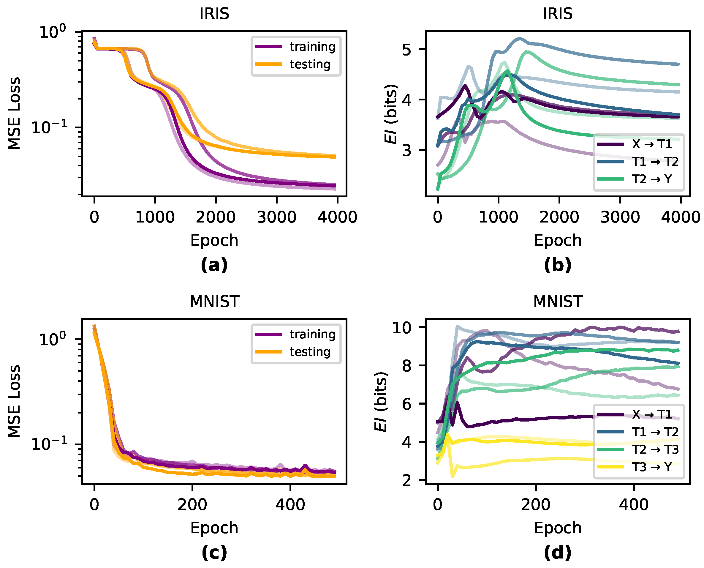
Qualitatively, we observe that the greatest changes in
significantly match the steepest parts of the loss curve during training and
is generally dynamic during periods of greatest learning (shown in
Figure 2). During the overfitting period when training performance dissociated from testing performance,
was generally flat across all layers, indicating that the information in the causal structure was unchanged during this period after the network had appropriately fitted.
4. Deep Neural Networks in the Causal Plane
As discussed in
Section 2,
depends both on the weight of connections as well as their degree of overlap, which together create the
manifold. This indicates that
can be decomposed into two properties: the
of the causal relationships represented by individual weights and the
of those relationships due to overlap in input weights. This mirrors previous decompositions of the
in Boolean networks or Markov chains into the determinism (here replaced with sensitivity, since neural networks are traditionally deterministic) and degeneracy [
16,
17]. This breakdown of
gives us more information than just whether
increases or decreases, but shows how the changes to its components lead to changes in the
, and how
reveals key properties of a DNN’s causal structure.
In DNNs, the of a layer measures how well the input transmits perturbations to the output nodes, while the of a layer measures how well the source of input perturbations can be reconstructed by examining the layer output. If the source of a perturbation cannot be reconstructed well the network is said to be degenerate. Together, these two dimensions of causal relationships form a “causal plane” which all DNN layers occupy. As layers differentiate via learning, their causal structures should occupy unique positions in the causal plane reflecting their contribution to the function of the DNN by becoming more sensitive or more degenerate.
To identify the position or trajectory of a DNN layer in the causal plane, both
and
are explicitly calculated based on the components of
. The
is calculated by summing the total contribution of each edge individually, in the absence of interaction effects between parameters. Therefore, the total
from layer
to the next layer
is
This is the same as calculating the of each (i,j) pair, but done independently from the rest of the network. Note that in a layer wherein each node receives only one unique input (i.e., no overlap) the is equal to the .
The
of a layer measures how much information in the causal relationships is lost from overlapping connections, and is calculated algebraically as
, as
measures the information contribution from non-overlapping connections in the network.
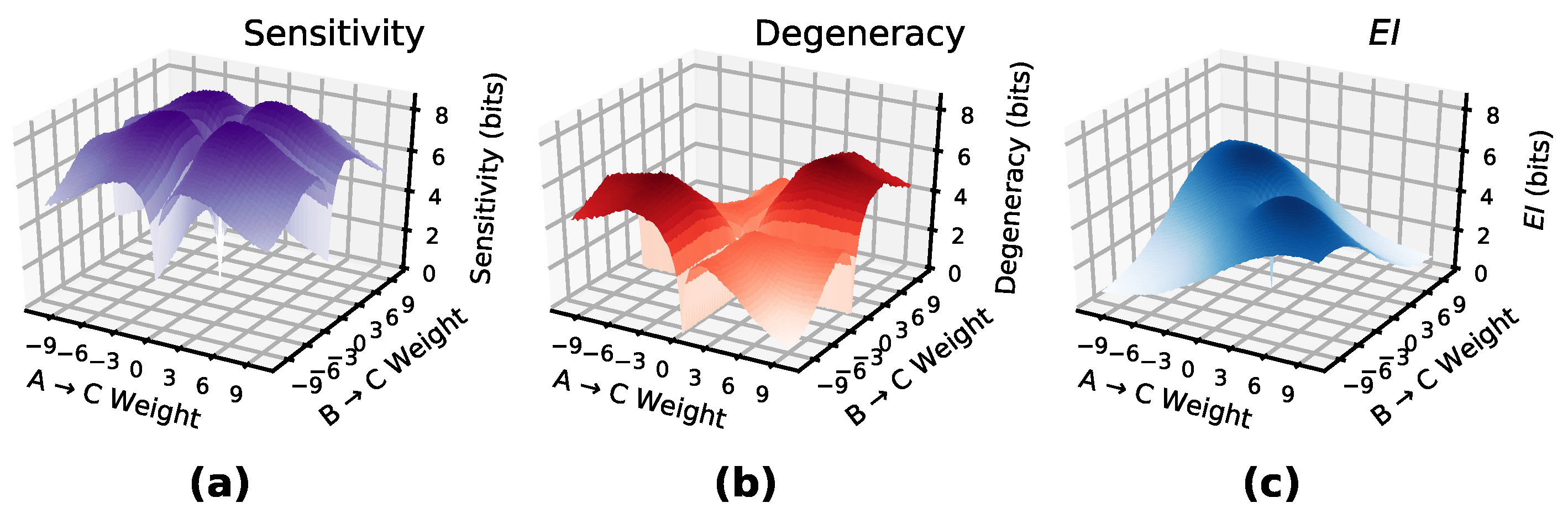
Figure 3 shows
and
manifolds for a layer of two input nodes and one output node (with sigmoid activations) with varying connection weights. The difference between them creates the
manifold.
Previous research investigating the
of graphs (based on random walk dynamics) has led to a way to classify different canonical networks, such as Erdős-Rényi random graphs, scale-free networks, and hub-and-spoke models, based on where they fall in terms of the determinism and degeneracy of random walkers [
17]. For
in DNNs a
term takes the place of determinism.
In order to visualize layer shifts between and we introduce the “causal plane” of a DNN, wherein the two dimensions of the plane represent the two respective values. The causal plane makes use of the fact that, as , if both increase equally, the itself is unchanged. When vs. is plotted, points on the line represent zero , and we refer to this line as the “nullcline” of the . Paths that move more towards sensitivity will increase , and paths that move more towards degeneracy will decrease , while paths along the nullcline will not change .
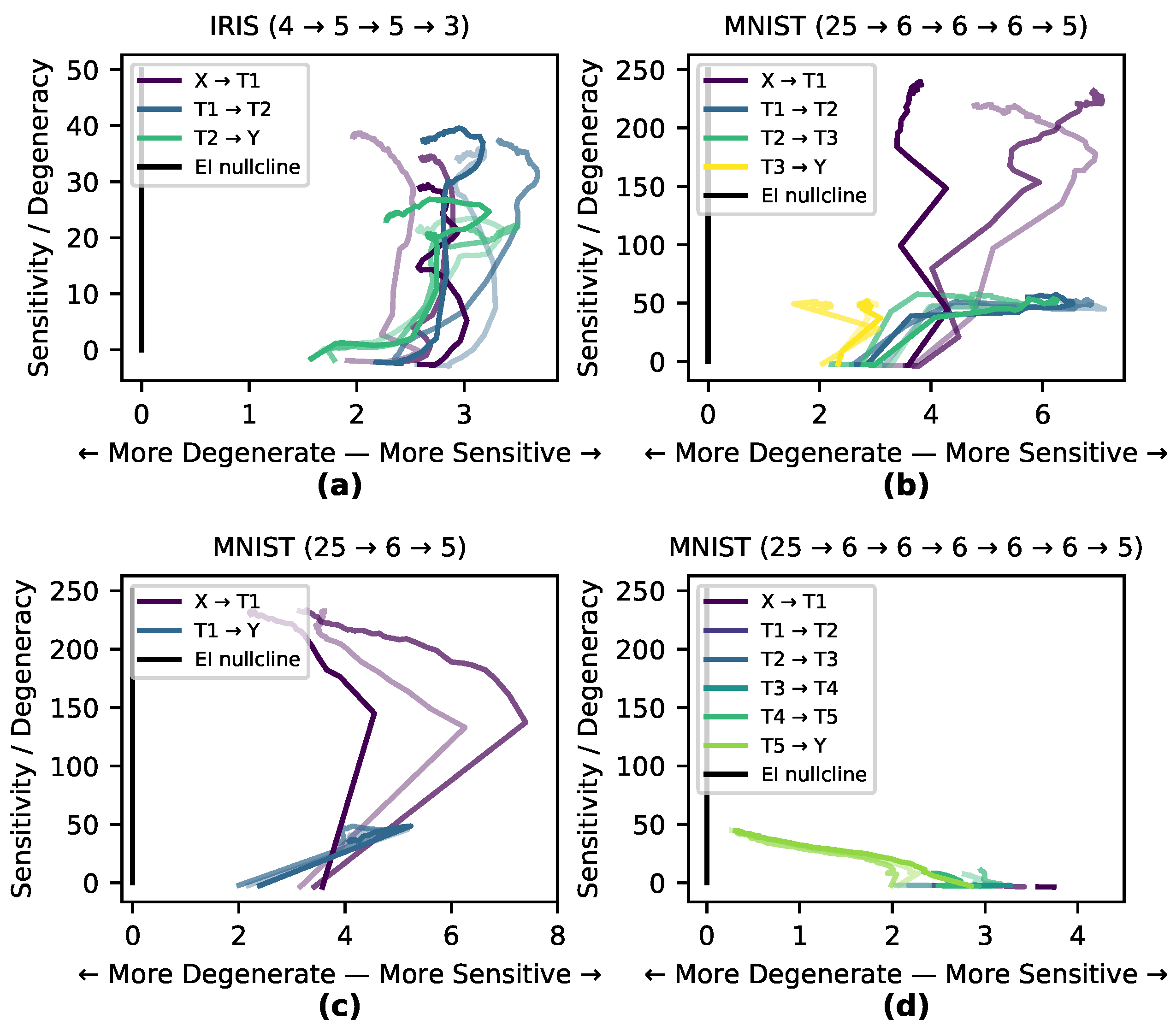
Here, we explore the hypothesis that the internal causal structure of a DNN shifts to match the task it is trained on, and that this happens in specific stages throughout the training process. To investigate this, we measured the paths of three runs on the Iris and MNIST data sets through the causal plane during training (shown in
Figure 4a–b). Of the two tasks, classifying MNIST digits is more degenerate and complex, as the network must transform a manifold in a high-dimensional space into only 10 distinct output classes (or rather 5 for our reduced version of MNIST here). The task of classifying Iris flowers is not as degenerate nor complex, as the network must transform a 4-dimensional space into three (mostly) linearly separable classes. If a network learns by matching its internal causal structure to the data set a network trained on MNIST would shape itself to a greater degree than one trained on Iris. This is precisely what we observe in
Figure 4 wherein the MNIST-trained network shows much greater differentiation and movement within the causal plane, while there is less differentiation in the causal structure of the Iris-trained network as it follows the
nullcline. In many cases, particularly for hidden and output layers, the runs first demonstrate an increase in sensitivity (increasing the
), and then later an increase in degeneracy (decreasing the
).
In order to examine the hypothesis that the causal structure of layers necessarily differentiate in response to training, the MNIST-trained network with sigmoid activation functions was modified in two ways: in one case a hidden layer was removed, and in the other case a number of redundant hidden layers were added (
Figure 4c–d). Both modifications of the network trained as accurately as the previous network. In the causal plane the added redundant layers moved very little, indicating a net-zero contribution to the
during training (for movie see
https://github.com/ei-research-group/deep-ei). This shows how redundant layers that don’t contribute to the network’s causal structure cluster along the
nullcline and move little, compared to more dynamic layers.
5. Measuring Joint Effects of Layer-to-Layer Connectivity
Integrated Information Theory (IIT) has been used to assess the total information contained in joint effects versus their independent effects in systems [
34]. It is a useful tool for causal analysis, analyzing the amount of information being integrated in a network’s causal structure [
35,
36]. Previously, the integrated information has been measured as the loss in
given a partition [
37], making
the upper bound for integrated information. However, there is no one accepted and universal measure of integrated information [
18,
38]. Instead, various measures for integrated information have been put forward in different systems [
39,
40]. Traditionally, the amount of integrated information in a feedfoward network is zero as there is no reentrant connectivity, as it is based on finding the minimum information partition across all possible subsets of a system. However, even in a feedforward network a layer’s nodes can still contain irreducible joint effects on another layer, and therefore we introduce a measure, feedforward integrated information, to apply in DNNs.
Normally calculating the integrated information requires examining the set of all possible partitions, which prohibits this method for systems above a small number of dimensions. Alternatively, in order to assess the synergistic contribution to
of individual edges, one would likely need to use multivariate information theory, such as the partial information decomposition, which grows at the sequence of Dedekind numbers as sources are included [
41].
In order to avoid these issues we introduce a measure,
, which is calculated based on contributions of each edge. That is, for each node
a sample
of its activation function under a maximum-entropy perturbation is recorded, along with that of each node
. To calculate
, each sample of each node is discretized into some shared chosen bin size, and the
of each (
i,
j) pair is calculated and summed:
Note that for a layer with a single node,
and
are identical. The same is true when each node of the network only receives a single edge. However,
measure will necessarily miss certain positive joint effects. Importantly, the difference between
and
measures can capture the amount of joint effects, and therefore the amount of information the layer-to-layer is integrating in a feedforward manner. Specifically, we compare
, the upper bound for integrated information, to
as defined in
Section 3, that is
. It should be noted that
, while designed to capture total joint effects of one layer to another, is not bounded by zero and can be negative. The sign of
determines if a network’s higher-order joint effects are informative or noisy. A network with a positive value of
will contain mostly informative joint effects, while a network with a negative value of
will contain mostly noisy joint effects. Note that its possible negative value makes it conceptually similar to the Interaction Information based on information decomposition [
42].
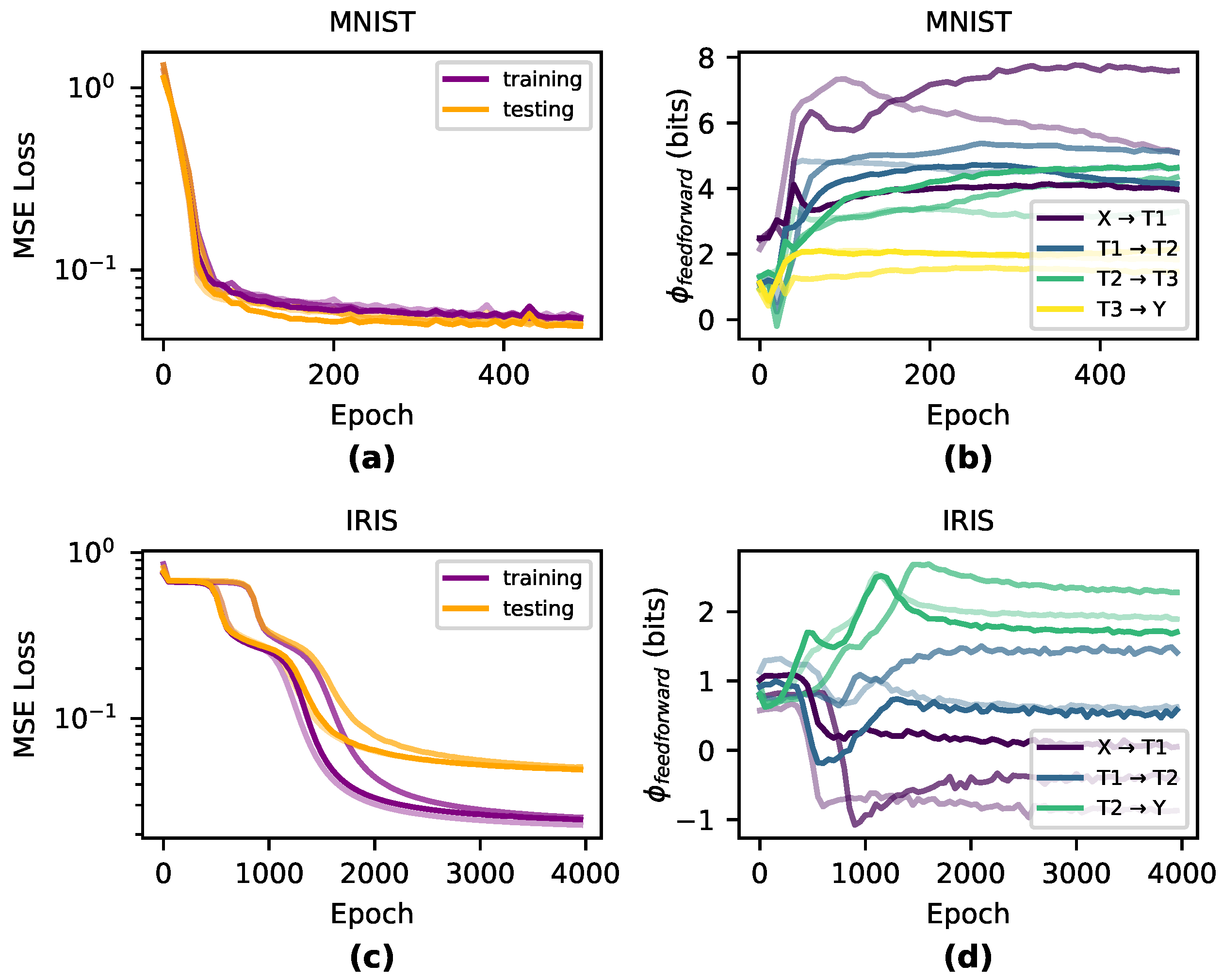
To understand how layer-to-layer joint effects change during training of a DNN, we analyzed how
changes during training across both Iris and MNIST data sets (see
Appendix A.1 for details on our methodology for measuring
). We observe that MNIST-trained networks have higher
than Iris-trained networks, indicating that the causal structure has indeed differentiated in accordance with the complexity of the task and requires more joint effects to learn (
Figure 5). This is likely because MNIST requires a more complex network than Iris and requires learning joint effects instead of the more linear learning for Iris.
6. Discussion
Here, we have introduced information-theoretic techniques to categorize and quantify the causal structures of DNNs based on information flows following perturbations. These techniques are built around the effective information (), which we adapted to apply to DNNs. It is defined as the mutual information following a set of perturbations of maximum entropy, and it reveals the information contained in the causal structure of a layer. For networks trained on both Iris and MNIST tasks, changed during the training period, particularly when learning actually occurred (as reflected by step changes in the loss function).
depends on both the and of a network. The between two nodes reflects the strength of causal relationships in isolation and peaks at particular characteristic weights for different activation functions (e.g., in sigmoid activation functions it peaks at e). The of a layer reflects the difficulty of downstream reconstruction of an upstream perturbation due to overlap of edge weights. Analyzing the reveals where networks lie on sensitivity/degeneracy space, which we call the “causal plane.” The ability to place network architectures in this plane means we can track how any given DNN’s causal structure evolves during its training as it moves through the space. Our results indicate that the causal structure of an DNN reflects the task it is trained on. For instance, in the MNIST task, different layers have a clear task in the causal structure of the DNN, reflected by each layer’s different trajectory in the causal plane, and adding new redundant layers added no new information to the causal structure by not contributing to the .
These techniques offer a different approach than work on information bottlenecks [
43], which is focused on using the mutual information to measure correlations between inputs and node activity. Both approaches have a similar goal to explain DNN generalizability and both share formal similarities, although here the focus is on the layer-by-layer causal structure itself rather than the input of DNNs. In the future, this work can be extended to different activation functions beyond the three considered here [
44,
45], unsupervised tasks [
46], recurrent neural networks such as LSTMs [
47], and convolutional neural networks [
2].
These techniques open up the possibility of assessing decompositions and expansions of the
, such as the integrated information of DNNs (as integrated information can be calculated using the minimum of
between subsets of a network [
15]), and integrated information is also decomposable into properties similar to
and
[
48]. Here, a measure of integrated information,
, is outlined that measures the irreducible joint effects in feedforward layer connectivity.
All of these may help understand why certain network architectures generalize and why some do not. In the future, these techniques also open the possibility for direct measurement of individual instances of causation in DNNs [
36].


