1. Introduction
The Pauli problem [
1] questions the possibility of deducing the theoretical quantum state (wave function) from the observed statistics of quantum measurements. The measurements are assumed to be ideal (i.e., infinitely accurate), and a reconstruction of the state, if at all possible, requires measuring several non-commuting operators (see for example [
2,
3,
4,
5,
6,
7] and Refs. therein).
Below we will consider the problem in a somewhat broader context. Quantum mechanics predicts probabilities of the outcomes of series of consecutive measurements by defining probability amplitudes for virtual histories (Feynman paths), followed by the system. The path amplitudes are then added, as appropriate, and the absolute square of the sum gives the probability of a particular scenario to occur [
8]. The measurements usually considered in connection with the Pauli problem are, in fact two-step sequences, consisting of preparing the system in an initial state and measuring the chosen variable later. The case of a preparation followed by two or more measurements made on the system is richer, since it allows for a different type of interference not available to the two-step histories.
In this paper we consider a different “Pauli problem”, namely the possibility of recovering the system’s path amplitudes from the results of intermediate fuzzy measurements, and discuss how it can be done in practice. The rest of the paper is organised as follows. In
Section 2 we revisit the basic rules for constructing probabilities with the help of virtual (Feynman) paths. In
Section 3 we apply the recipe of
Section 2 to a composite
system +
probe, and explain why the two-step histories are insufficient for our purpose. In
Section 4 we extend the approach to three-step histories where a system is “pre- and post-selected” in known initial and final states. In
Section 5 and
Section 6 we apply the method to the simplest case of a two-level system (a qubit), and in
Section 7 provide a numerical simulation.
Section 8 discusses the “strong” and “weak” limiting cases where the approach of
Section 4,
Section 5,
Section 6 and
Section 7 fails, and analyses the reason for the failure. In
Section 9 we evaluate the “strong” and “weak” averages of the pointer’s readings, and briefly comment on the popular subject of the so-called “weak measurements” [
9]. Usefulness of the paths amplitudes for predicting the outcomes of future measurements, and making statements about the system’s past is analysed in
Section 10.
Section 11 contains our conclusions.
2. From Amplitudes to Probabilities
We start by recalling the rules for evaluating the probabilities of three consecutive measurements, given in [
8], and recently revisited in [
10,
11,
12]. Consider such measurements performed on a quantum system (
s), with which one associates a
N-dimensional Hilbert space,
. Three quantities, represented by operators
,
, are measured at
,
, and
, respectively. Each operator has
possibly degenerate eigenvalues,
,
, and can be written as
where
,
form a suitable orthonormal basis, and
for
, and 0 otherwise.
To be able to define a statistical ensemble, one needs the first measurement to yield a non-degenerate eigenvalue
, which prepares the system in the corresponding state
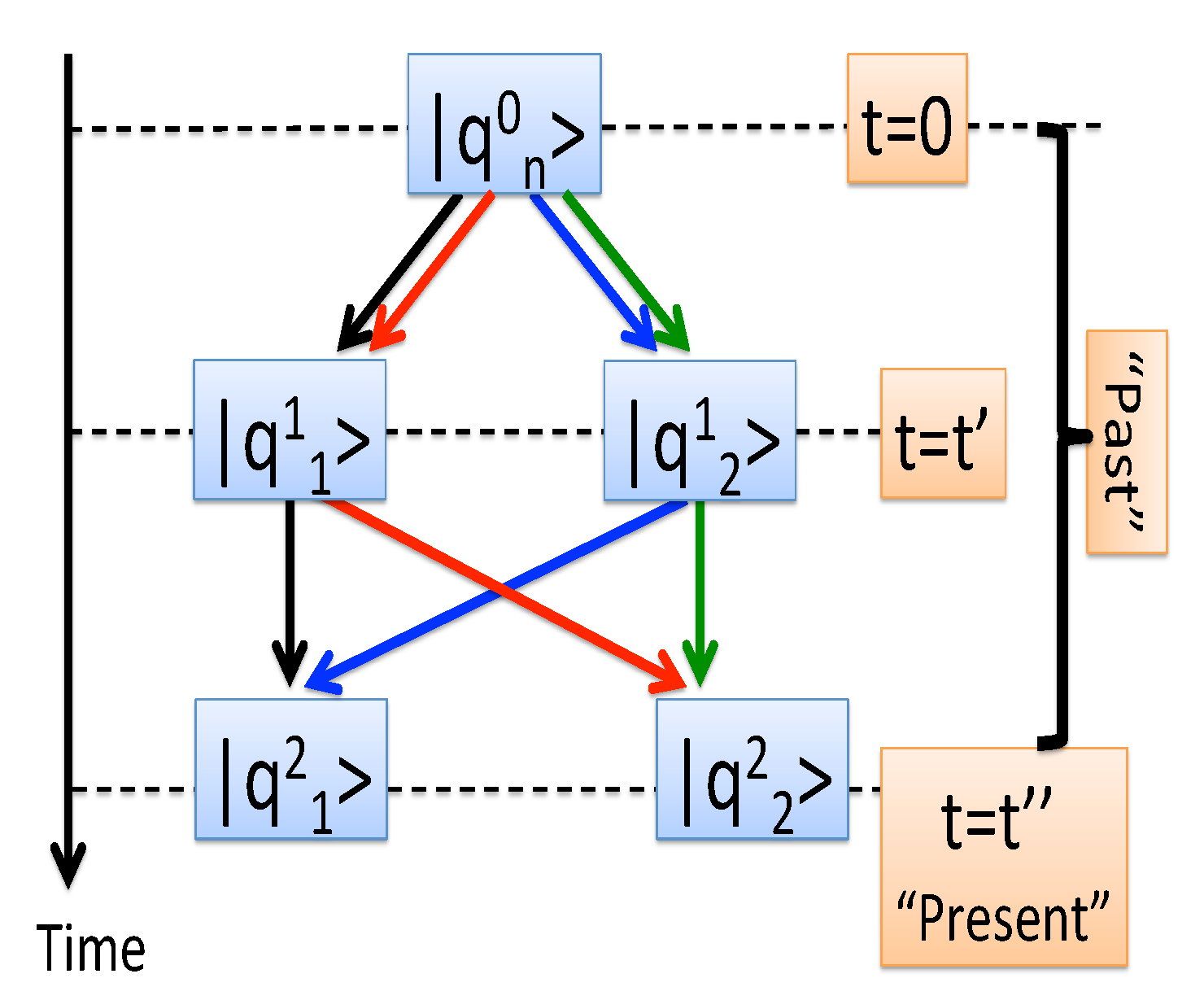
. The next step consists of evaluating the
probability amplitudes for all virtual (Feynman) paths,
, starting at
and passing through all possible states at
and
(see
Figure 1),
where
is the system’s evolution operator. An amplitude for obtaining at
a value
is found by summing (
2) over all states
, consistent with
,
,
Finally the
probability for having a sequence of observed outcomes
is found by summing absolute squares of the amplitudes (
3) over the degeneracies of the last eigenvalue
,
Two relevant observations can be made here. Firstly, the scheme is explicitly causal in the sense that future observations cannot affect the statistics of the ones already made. In particular, summing (
4) over all outcomes
restores the probabilities for the experiment in which only
and
are measured,
For someone interested in the statistics of only the first two measurements it does not, therefore, matter what would be measured at , or if anything would be measured in the future at all.
Secondly, the scheme treats the “past” (any
) and the “present” (at
) differently. If the measured eigenvalue is degenerate, in the “past” one sums the amplitudes, as in Equation (
3). At “present”, the probabilities
are added, as in Equation (
4). The latter rule [
8] can be traced to the need to ensure causality in the case an operator commuting with
and having
N distinct eigenvalues is measured in the immediate future at
,
[
10].
The rules, although formulated for systems in a finite-dimensional Hilbert space are readily generalised to the case where the measured operators have continuous spectra. Note also that they can be used to obtain more compact expressions for the probabilities (
5) in terms of the projectors onto the eigen-subspaces of the chosen operators (see, e.g., Section 2.2 of [
12]).
3. Von Neumann Measurements and the Two-Step Histories
The standard approach to quantum measurements involves coupling the system of interest to another degree of freedom (a probe), and deducing the system’s properties from the probe’s statistics. One choice of a probe is a von Neumann pointer (
p) [
13], a one dimensional free particle of a mass
M with a coordinate
f and a momentum
. The pointer is briefly coupled to the system (
s) at some
, so that the full Hamiltonian is given by
where
refers to the system, the operator
represents the system’s variable to be measured, and
is the Dirac delta. We will start by assuming that all eigenvalues of
,
,
are different, and return to degenerate
’s at the end of the next Section.
A possible experiment consists of preparing the composite
{system+
pointer} in a known initial state measuring
, applying the coupling (
6), and then making a measurement on the pointer,
. The purpose of the experiment is to learn something about the system in the absence of the probe. We, therefore, have a two-step history, which can be treated by the method of
Section 2. At
the system and the pointer are prepared in states
and
, respectively. In particular, we suppose that the outcome of
is
, so
with
and
acts only on the pointer.
Thus, obtaining an outcome
one prepares the composite in an initial state
In what follows, we will assume
to be a real symmetric Gaussian,
where the width
determines the uncertainty in the pointer’s
initial position and, therefore, affects the accuracy of the measurement.
To describe the pointer at we will use a continuous basis , , and the measured operator, , with a discrete spectrum , . Thus, after observing an outcome one knows that the (yet undefined) variable has a value in an interval . The newly introduced parameter determines the accuracy with which the pointer is read. Note that an eigenvalue is highly degenerate, since , for any , and .
The evolution operator for the composite {
system +
pointer} is a product
where
, and
.
Following the recipe of
Section 2 we write down the probability amplitudes for all virtual (Feynman) paths
in the composite’s Hilbert space,
,
where
is the systems transition amplitude [
8] between the states
and
, defined in the absence of the pointer, and the factor
can be written as
since
.
With only two measurements, all paths
lead to distinguishable (orthogonal) final states, and the probability to have a pointer reading
is found by adding absolute squares of the amplitudes (
13)
Therefore, regardless of how accurately the meter was prepared and read, all information about the phases of the amplitudes
is lost. This is because, according to the rules of
Section 2 none of the virtual paths are allowed to interfere. For someone still wishing to determine the system’s initial state
, the standard way to proceed is to choose a different operator
,
repeat the measurement, and use the obtained data [
2,
3,
4,
5,
6,
7]. We will, however, consider a different problem, in order to exploit the interference associated with the measurements made in the “past”.
4. From Probabilities to Amplitudes. Three-Step Histories
Suppose next that an additional measurement is made on the system at a . Now the measurement made on the pointer at belongs to the past, and a different rule will apply.
The new experiment is as follows. At
the system and the pointer are prepared in a state
, and coupled according to (
6) just before
. At
, a measurement made on the pointer yields an outcome
. At
the outcome
is recorded, but only if a measurement
made on the system at
yields a particular outcome
. The three steps are repeated enough times to evaluate the probabilities of having an outcome
, given a later outcome
. The purpose of the experiment is to recover the values of the system’s amplitudes, defined in the absence of the pointer.
This is a three-step measurement, for which we have
We will assume the eigenvalues
to be non-degenerate provided
is acting in the Hilbert space
of the system. They are, however, highly degenerate, if
acts the
, since
, for any
.
Next we apply the rules of
Section 2. Evaluating the amplitudes for all virtual paths in
, connecting
with
, and
with
[cf. Equation (
2)], we find
where
is the amplitude for the system to follow a path
in
.
Summing the amplitudes over the degeneracies of the operator
acting in the
[cf. Equation (
3)], yields
Finally, summing over the degeneracies of
in the
[cf. Equation (
4)], we have
where
is the overlap matrix of the pointer’s states,
and
is the probability density of the pointer’s readings, obtained for a system ending up in
at
(see
Appendix A).
The measured system contributes to
with the path amplitudes given in (
21), whose values can, in principle, be determined by rewriting Equation (
23) in an equivalent form,
where
The system of linear equations (
25) can be solved if the probabilities
have been measured for
different intervals
,
. Solving Equation (
26) for
and
,
, one will be able to determine the values of all amplitudes
up to an unimportant overall phase.
To conclude the Section, we note that the measured operator
may have
degenerate eigenvalues,
where
projects onto its
j-th eigen-subspace. In this case the analysis remains the same, except that
N is replaced by
J, and the
J amplitudes to be determined,
result from the interference between the virtual paths (
21) not distinguished by a measurement of
.
Next we see how the scheme would work in the simplest case of a two-level system, .
5. An Inverse Measurement Problem
We can write Equation (
23) as
where
is a complex “vector” with the components
,
, and
is an “operator” with matrix elements
,
, and the subindex
accounts for the specific subset of intervals used. The problem now takes a more familiar form. One needs to find the components of a (fictitious) state
, given the expectation values of the hermitian operators
,
.
Equationation (
29) is particularly useful in the case
, where
can be seen as an unnormalised state of a fictitious “spin”, and
can be expanded in terms of the Pauli matrices (
,
,
, and
),
with four intervals
corresponding to the pointer’s readings
, chosen at one’s convenience. The resulting four equations (
29) determine the “spin”’s projections
onto the three spatial axes, as well as the state’s norm,
,
The polar angles
and
of the axis along which the “spin” is polarised,
determine the “spin”’s state
up to an arbitrary overall phase and, returning to our original notations, we have the desired result,
Next we see how the scheme will work in practice.
6. Double-Slit Interference
It is natural to start with the simplest case, where one measures the final position of a massive pointer,
, and
which moves only when it interacts with the system, and whose state remains the same once this interaction is over [
13]. If so, the matrices
are real,
and the coefficient multiplying
in Equation (
30) vanishes,
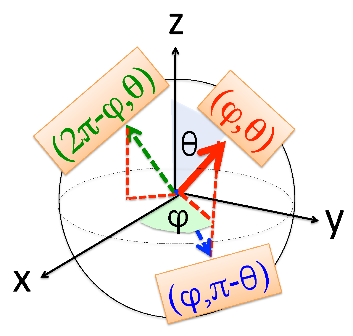
. One can still solve any three of Equation (
31) for
,
, and
but would be unable to decide between
and
, as illustrated in
Figure 2. (Note that the problem is exacerbated for
where
signs would remain indeterminate when calculating the relative phases.)
Measuring instead the final pointer’s momentum
,
, one encounters a similar difficulty. In this case we have
so that
, and having solved the three remaining equations one will not be able to decide between
and
(see
Figure 2).
However, provided both
and
have been measured independently in two different experiments, one can combine the results to obtain the four Equation (
31). For example, choosing any three equations employing
and
, and one using
and
, will determine the two amplitudes (
33) unambiguously (up to a global phase).
Finally we note that the case of a two-level system is conceptually similar to a Young’s double-slit experiment. Here the two states and play the roles of the two holes, and the target state , together with its orthogonal companion, , are the “points on the screen”. Unperturbed probabilities and correspond to having an “interference pattern on the screen”. Thus, if a von Neumann measurement perturbs the interference pattern (the probability to be detected in is ), yet does not destroy it completely, and the values of the path amplitudes can be deduced from the measurement’s statistics.
7. A Simple Example
To see the efficiency of the proposed scheme, we first change it a little. It is possible to avoid mixing the results of measuring the pointer’s position and momentum, if the condition (
34) is relaxed, and the pointer’s initial state
is allowed to spread in the coordinate space. Choosing
, from (
15) we have
The appearance of a “complex width”
allows one to determine all coefficients
in Equation (
30) from the statistics of the final pointer’s positions. Explicitly, from (
24) we have
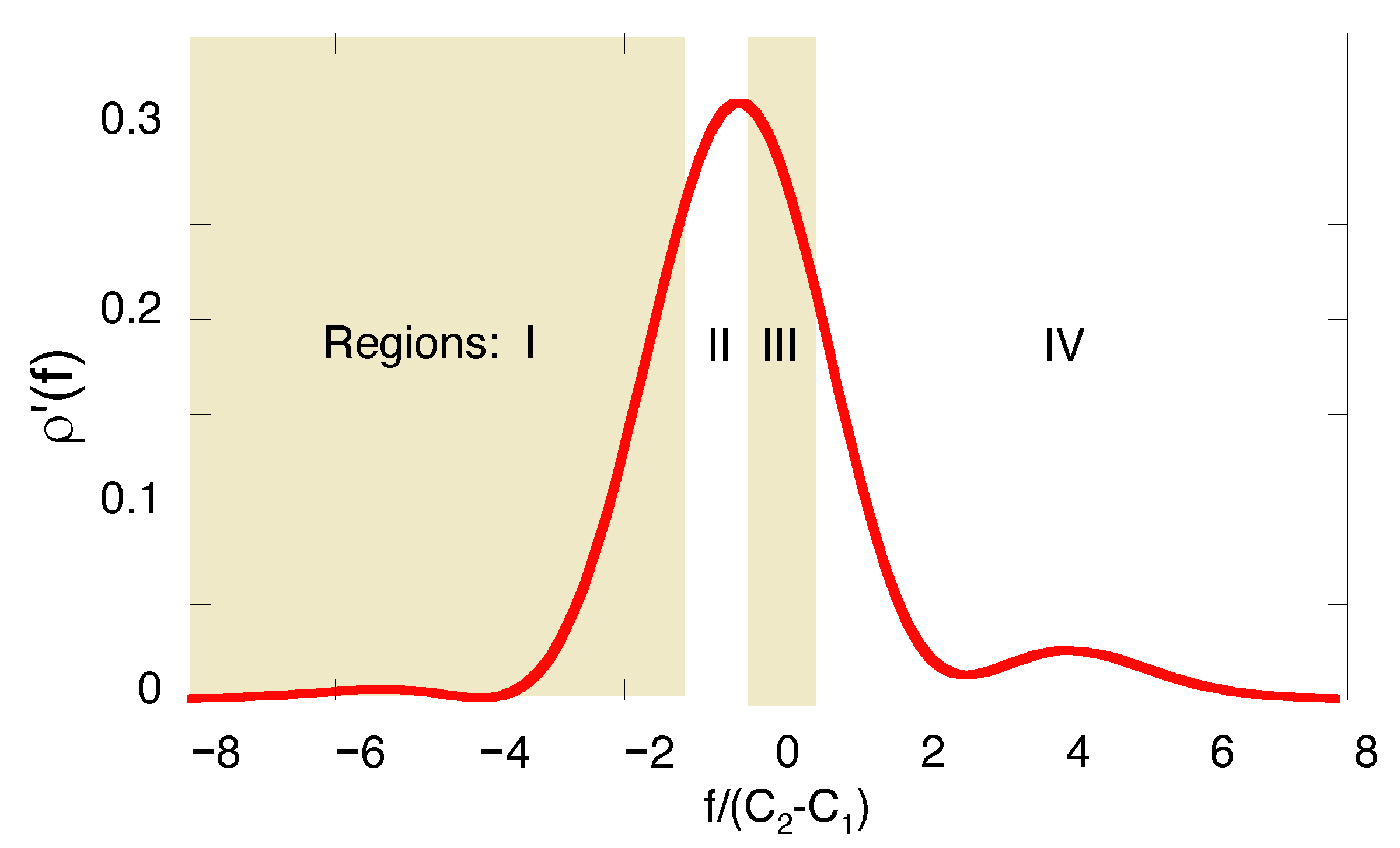
In an actual experiment set-up to evaluate the amplitudes
a successful post-selection of the system in the final state,
, will occur
K times out of the total number of trials,
. It is convenient to divide the full range of
f into four regions,
,
, each containing a quarter of all cases,
(see
Figure 3). To simulate the measurements, we use a random number generator, obtain four numbers
,
,
, and
,
, replace the probabilities in the r.h.s. of Equation (
31) by their estimates,
and solve Equation (
39) for different values of
.
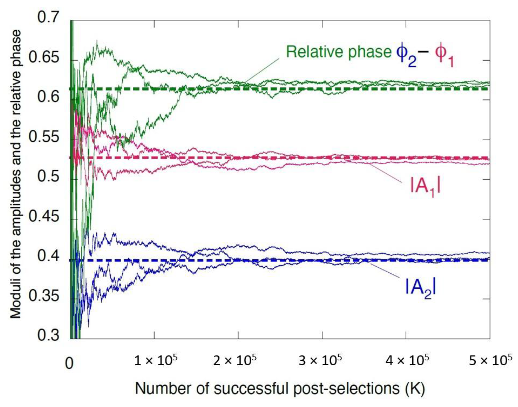
The results of three simulations for
arbitrarily chosen (unnormalised) initial and final states,
and
are shown in
Figure 4. It takes approximately
successful post-selections in order to recover the amplitudes of
, given the values in Equation (
42). Next we discuss the two limiting cases, in which the method of this Section will fail.
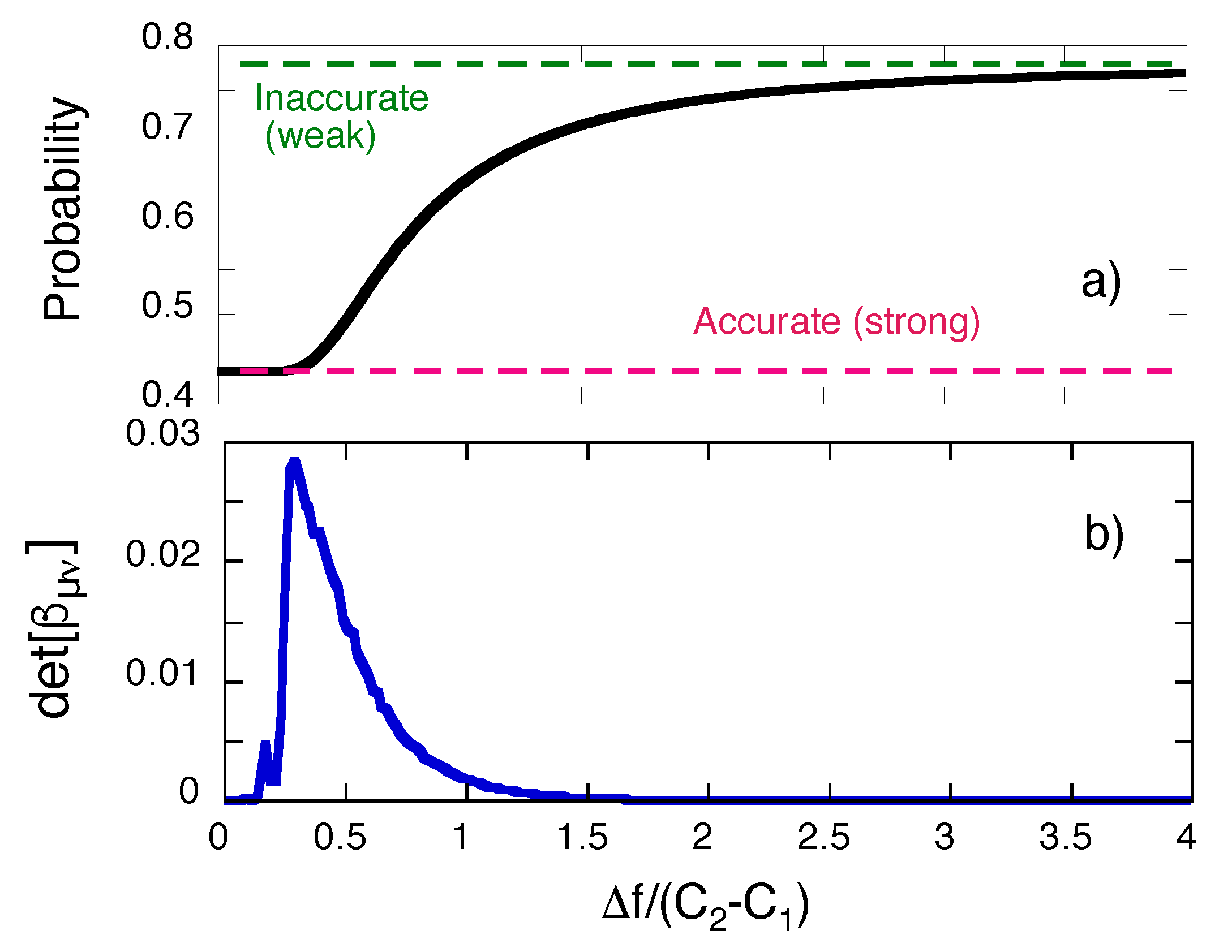
8. Accurate (Strong) and Inaccurate (Weak) Limits
The method of
Section 8 fails, or at least becomes impractical as
or
. The uncertainty in the initial pointer’s position determines the perturbation suffered by the measured system, as shown in
Figure 5a, where the probability of detecting the system in the final state
,
is seen to vary from
to
, as
increases from 0 to ∞. In both limits the matrix in the l.h.s. of Equation (
39) becomes singular, as shown in
Figure 5b.
In particular, if the initial position of the pointer is highly uncertain,
, from (
23) we have
The pointer decouples from the system, and the interference between the two virtual paths is preserved,
Note that the same effect can be achieved by leaving the width
constant, and multiplying the coupling term in Equation (
6),
, by a constant
. Indeed, scaling the pointer’s coordinate by choosing
, would result in
If, on the other hand, the initial position of the pointer is known accurately,
, Equation (
23) yields
since by (
15)
Thus, an accurately set pointer strongly perturbs the system by completely destroying interference between the virtual paths, even when the spreading of its initial state is taken into account.
9. Averages and the “Weak Measurements”
Another possibility to explore the limits
and
is to evaluate the moments of the distribution of the pointer’s readings (
23),
These are, of course, also expressed in terms of the system’s path amplitudes
, and we will look at the
’s first moments in the “strong” and the “weak” limits. For simplicity, we will restore the condition (
34) or, what is the same, assume that the times
and
are so short that
.
Expansions around
are not particularly interesting. Bearing in mind that
, in the two-level case of
Section 6, for
we have
where
is the average, obtained in a highly accurate measurement, and the factors
and
, which only depend on the parameters of the pointer and the eigenvalues
, rapidly decrease for
(See
Appendix B).
Similarly, since
, for the mean pointer’s momentum,
we obtain
where
is given in the Appendix B. Thus, some information about the relative phase of the two path amplitudes can be obtained from accurate yet not too accurate measurements. However, the expressions (
50) and (
51) are cumbersome and, as we already said, not particularly interesting.
The opposite limit
is involved in the controversy surrounding the so-called “weak measurements”. Returning to the notations of
Section 3 and noting that
, for the pointer’s mean position we have
Similarly, for the mean pointer’s momentum we find
where
is the variance of the distribution of the momenta in the initial pointer’s state
,
which vanishes when
becomes very broad in the coordinate space, and
.
Equationations (
50)–(
53), although different, illustrate the same point. Any average, evaluated for a pointer coupled, as in Equation (
6), to a system making a transition between initial and final states will have to be expressed in terms of certain combinations of the system’s transition amplitudes, defined in the absence of the pointer. Transition amplitudes are the basic elements of the description of quantum motion [
8], and this is really all that can be said about this matter.
The above analysis relates to the so called “weak values” WV(for a recent review see [
9]). For short enough
and
,
, the quantity in the square brackets in Equations (
52) and (
53) reduces to a ratio of matrix elements
Presented in this manner in [
14], the r.h.s of Equation (
55) was dubbed “the weak value of
for a system pre- and post-selected in its initial and final states”, which be can obtained in a particular kind of “weak quantum measurements”. Various weak values have been measured experimentally, yet their place and status within conventional quantum mechanics remain unclear. We have long advocated the interpretation of the “weak measurements” in terms of Feynman’s transition amplitudes, and refer the reader to [
15,
16,
17,
18] for an analysis of the role of the Uncertainty Principle and the significance of “anomalous weak values”. Here we further support this view by placing the “weak measurements” within a broader context of measuring the transition amplitudes, absent in the simple two-step histories of
Section 2.
10. Prediction and Retrodiction
Having recovered the transition amplitudes
, it is reasonable to question the usefulness of what has been found. If the amplitudes are known for all
,
, they can be used to predict the results of other measurements made on the same system staring in the same
, and ending in the same
, provided the new operator
commutes with
,
. Indeed, their values is all that required to compute the probabilities
in Equation (
23), for any choice of
,
,
and
, even if the Hamiltonian of the system,
, is not known. The task is not entirely trivial for
, where
can have degenerate eigenvalues, and the corresponding amplitudes must be added, as described in
Section 2.
On the other hand, little can be learnt about an intermediate measurement of a
which does not commute with the
. This is seen already from the
example, discussed in the previous Section. Suppose one replaces
with a
, so that now
and
Of the four quantities in the r.h.s. of Equation (
57) needed to evaluate
, only the first two are known from measuring the
, and this is clearly not enough.
Another use of the path amplitudes (
21) and (
28) is retrodictive reconstruction of the system’s past. Classically, the knowledge of a system’s current position, velocity, and its Lagrangian is sufficient for predicting its position in the past. Quantally, one may wish to determine the system’s initial state,
, from the values of the path amplitudes. The state is fully determined by the coefficients
of its expansion in some known basis
,
. If the system’s Hamiltonian
is known, the operator
has non-degenerate eigenvalues [cf. Equation (
7)], and the values of
have been measured, the problem is easily solved. Indeed, using (
21) we obtain
and with
thus determined, the results of other possible measurements can be predicted.
However, if some of the
’s eigenvalues are degenerate [cf. Equation (
27)], full reconstruction of the initial state is not possible, since important information is lost to interference. From (
28) we have
so that the values of
cannot be recovered from the known values of
.
11. Conclusions
In summary, we have shown that the values of system’s transition amplitudes can be deduced from the statistics of an intermediate measurement. The deduction is possible provided the measurement is “fuzzy”, and does not destroy interference between the system’s virtual paths. What distinguishes our method from usual approach to the “Pauli problem” [
2,
3,
4,
5,
6,
7] is its reliance on a type of interference, absent in two-step histories, consisting only of preparation and the actual measurement. With the post-selection step added, the situation is conceptually similar to a double-(multiple-) slit experiment [
8], in which a probe, designed to determine the path taken by the system, does its job imperfectly, so a vestige of the interference pattern is retained on the screen. There is a two-way relationship between a result of observation and what can be considered a computational tool, although it is typically more difficult to deduce amplitudes from the probabilities than to construct the probabilities from the known amplitudes.
Finally, it is worth noticing that neither reconstructing the amplitudes as in
Section 7, nor evaluating their combinations by measuring the “weak values” of
Section 9, would serve to provide a deeper insight into quantum mechanical formalism. If asked “what has been evaluated?” one can only answer “amplitudes”. Moreover, if asked further “what are these amplitudes?” one can only reply “something quantum theory uses to predict the observable probabilities”.


