Transitional Channel Flow: A Minimal Stochastic Model


Abstract
1. Context
1.1. Physical Context: Plane Channel Flow
1.2. Modeling Context: Directed Percolation, Probabilistic Cellular Automata, and Criticality Issues
2. Description of the Model
2.1. Context
2.2. Design of the Model
- 1.
- corresponds to the natural propagation of the active state along its own motion direction. Accordingly, the active site B at is expected to be found at and time with a high probability, , which corresponds to the near-deterministic propagation of an active state as observed for . With probability , site will not turn active, which means that the LTB has decayed or experienced a speed fluctuation that delayed its propagation. The corresponding R configuration is .
- 2.
- Configuration corresponds to an active site B at that is not supposed to stay in place but move to with probability and leave site empty at time . The probability that is still active at time , therefore, generally corresponds to the creation of a novel active state by in-line longitudinal splitting at the rear of the active state that has effectively moved. Persisting activity at and time can also be the result of state at and time t experiencing a speed fluctuation leaving it stuck at the same place with probability as argued above for configuration . The presence of parameter undoubtedly makes the dynamics richer. The corresponding R-configuration is .
- 3.
- Configuration corresponds to an active state B at site that contaminates backwards and laterally upstream the site at in addition to its likely propagation to with probability . This is precisely what is sometimes observed for longitudinal splitting, where the daughter follows a track parallel to that of the mother but slightly shifted upstream, i.e., off-aligned. Configurations and both account for longitudinal splitting but the latter hence introduces some lateral diffusion. Along this line of thought, numerical simulation results in [14], illustrated in Figure 4, suggest that probability is tiny close to but increases with . The corresponding R-configuration is .
- 4.
- In configuration , the active site B at is supposed to advance further at with probability . Persisting activity at , therefore, means longitudinal splitting ahead but now with the opening of a wide laminar gap between the offspring left behind at and the parent that has advanced, with probability , at . Else, activity at and could result from activity at and time t propagating backwards to at time . These circumstances have not been observed and appears unlikely or impossible, which suggests to take . The corresponding R-configuration is .
- 5.
- In configuration , the state B at and time t is expected to be at at time . State at being active at means contamination backwards and laterally downstream, which is never observed in the simulations; hence, . The corresponding R-configuration is .
- 6.
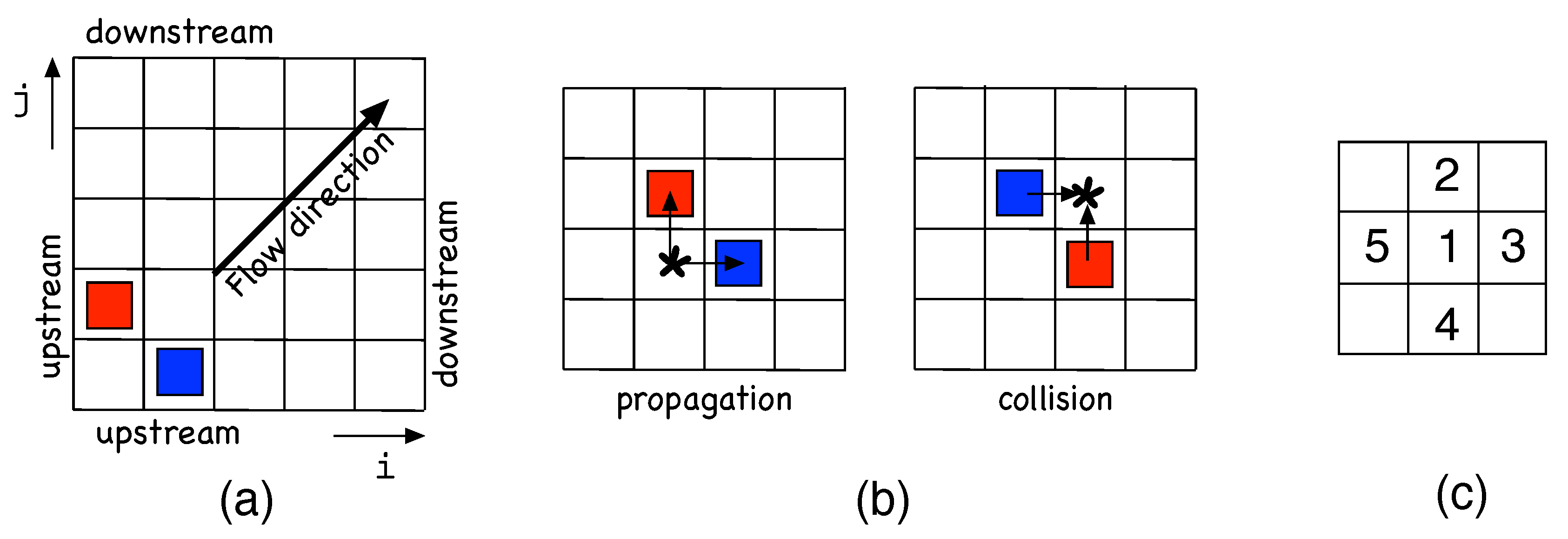
- Still about configuration , the situations described in the previous items all imply single-colored evolution, which is guaranteed below the onset of transversal splitting, i.e., . When , as illustrated in Figure 3, this splitting produces an R offspring at out of a B parent at or B offspring from an R parent at , as sketched in Figure 7 (left). A probability will be associated with it, where the prime is meant to recall that it involves states of different colors.
- 7.
- When the general expression (3) gives non-zero probabilities to and the resulting superposition of states is not allowed and a choice has to be made. It might seem natural to keep the state with the maximum probability but, depending on circumstances hard to decipher, collisions sometimes appear to cause the decay of both protagonists or else reinforce the dominance of one color in a given region of space. A similar bias can affect transversal splitting. These peculiarities are not taken into account here: for simplicity, in all conflicting cases, we make the assumption that the result is non-empty and random with probability .
2.3. Mean-Field Approach
2.4. Numerical Simulations
3. Before Onset of Transversal Splitting,
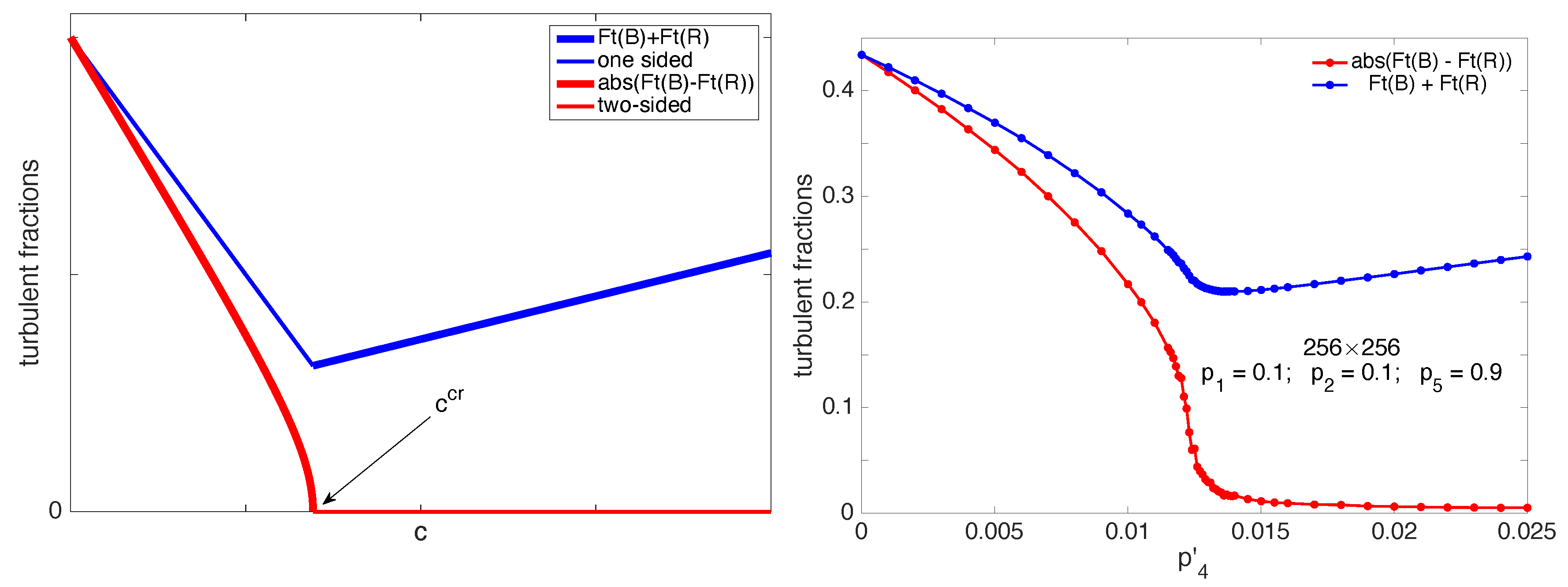
3.1. Coarsening from Two-Sided Initial Conditions
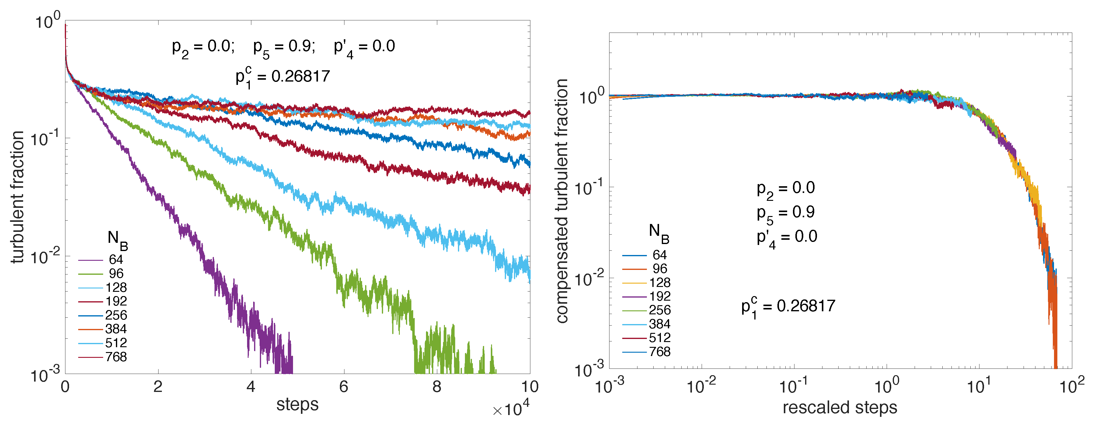
3.2. Decay: 1D vs. 2D
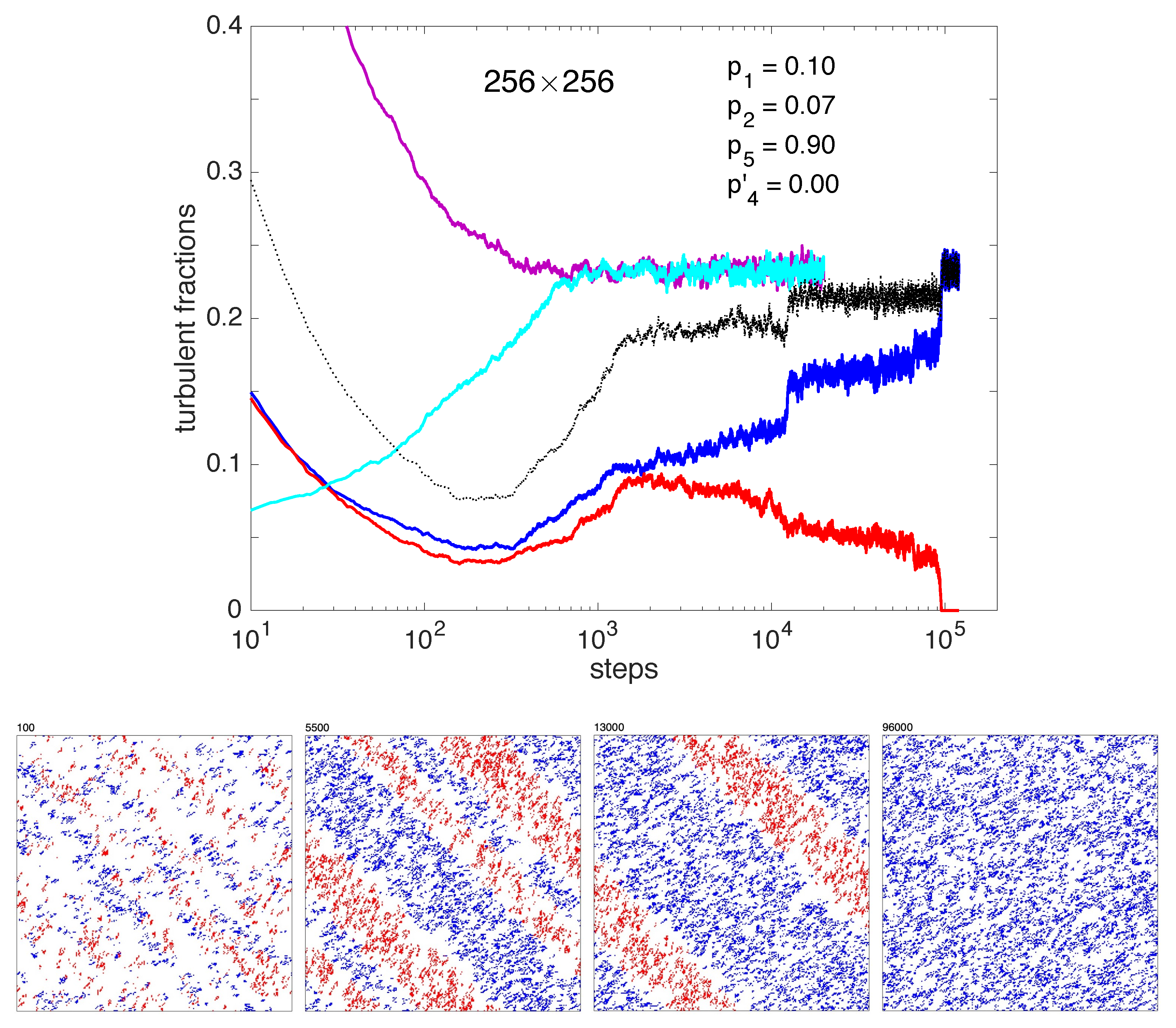
4. Beyond Onset of Transversal Splitting,
5. Discussion and Concluding Remarks
Author Contributions
Funding
Acknowledgments
Conflicts of Interest
Abbreviations
| 1D/2D/3D | One/two-dimensional (depending on 1/2 space coordinates) |
| DP | Directed percolation (stochastic competition between decay and contamination) |
| LTB | Localized turbulent bands |
| DAH | downstream active head (part of an LTB controlling its propagation) |
| PCA | Probabilistic cellular automata |
| CML | Coupled map lattice (spatially-discrete iterative model) |
References
- Pomeau, Y. Front motion, metastability and subcritical bifurcations in hydrodynamics. Phys. D 1986, 23, 3–11. [Google Scholar] [CrossRef]
- Hinrichsen, H. Non-equilibrium critical phenomena and phase transitions into absorbing states. Adv. Phys. 2000, 49, 815–958. [Google Scholar] [CrossRef]
- Manneville, P. Transition to turbulence in wall-bounded flows: Where do we stand? Mech. Eng. Rev. Bull. JSME 2016, 3. [Google Scholar] [CrossRef]
- Tuckerman, L.S.; Chantry, M.; Barkley, D. Patterns in Wall-Bounded Shear Flows. Annu. Rev. Fluid Mech. 2020, 52, 343–367. [Google Scholar] [CrossRef]
- Lemoult, G.; Shi, L.; Avila, K.; Jalikop, S.V.; Avila, M.; Hof, B. Directed percolation phase transition to sustained turbulence in Couette flow. Nat. Phys. 2016, 12, 254–258. [Google Scholar] [CrossRef]
- Chantry, M.; Tuckerman, L.S.; Barkley, D. Universal continuous transition to turbulence in a planar shear flow. J. Fluid Mech. 2017, 824, R1. [Google Scholar] [CrossRef]
- 73rd Annual Meeting of the APS Division of Fluid Dynamics. Sessions Y03 and Z10. 2020. Available online: https://dfd2020chicago.org/ (accessed on 27 November 2020).
- Waleffe, F. On a self-sustaining process in shear flows. Phys. Fluids 1997, 9, 883–900. [Google Scholar] [CrossRef]
- Kaneko, K. Overview of coupled maps. Chaos 1992, 2, 279–283. [Google Scholar] [CrossRef]
- Bottin, S.; Chaté, H. Statistical analysis of the transition to turbulence in plane Couette flow. Eur. Phys. J. B 1998, 6, 143–155. [Google Scholar] [CrossRef]
- Vanag, V.K. Study of spatially extended dynamical systems using probabilistic cellular automata. Phys. Uspekhi 1999, 42, 413–434. [Google Scholar] [CrossRef]
- Kashyap, P.V.; Duguet, Y.; Dauchot, O. Flow Statistics in the Transitional Regime of Plane Channel Flow. Entropy 2020, 22, 1001. [Google Scholar] [CrossRef]
- Gomé, S.; Tuckerman, L.S.; Barkley, D. Statistical transition to turbulence in plane channel flow. Phys. Rev. Fluids 2020, 5, 083905. [Google Scholar] [CrossRef]
- Shimizu, M.; Manneville, P. Bifurcations to turbulence in transitional channel flow. Phys. Rev. Fluids 2019, 4, 113903. [Google Scholar] [CrossRef]
- Manneville, P.; Shimizu, M. Subcritical Transition to Turbulence in Wall-Bounded Flows: The Case of Plane Poiseuille Flow. Rencontre du Non-Linéaire, Paris. 2019. Available online: http://nonlineaire.univ-lille1.fr/SNL/media/2019/CR/ComptesRendusRNL2019.pdf (accessed on 27 November 2020).
- Shimizu, M.; Manneville, P. Onset of sustained turbulence and (1+1)D directed percolation in channel flow. In Proceedings of the Annual Meeting of Fluid Mechanics Society of Japan, Tokyo, Japan, 13–15 September 2019. [Google Scholar]
- Seshasayanan, K.; Manneville, P. Laminar-turbulent patterning in wall-bounded shear flow: A Galerkin model. Fluid Dyn. Res. 2015, 47, 035512. [Google Scholar] [CrossRef]
- Chantry, M.; Tuckerman, L.S.; Barkley, D. Turbulent–laminar patterns in shear flows without walls. J. Fluid Mech. 2016, 791, R8. [Google Scholar] [CrossRef]
- Barkley, D. Theoretical perspective on the route to turbulence in a pipe. J. Fluid Mech. 2016, 803, P1. [Google Scholar] [CrossRef]
- Allhoff, K.T.; Eckhardt, B. Directed percolation model for turbulence transition in shear flows. Fluid Dyn. Res. 2012, 44, 031201. [Google Scholar] [CrossRef]
- Sano, M.; Tamai, K. A universal transition to turbulence in channel flow. Nat. Phys. 2016, 12, 249–253. [Google Scholar] [CrossRef]
- Kreilos, T.; Khapko, T.; Schlatter, P.; Duguet, Y.; Henningson, D.S.; Eckhardt, B. Bypass transition and spot nucleation in boundary layers. Phys. Rev. Fluids 2016, 1, 043602. [Google Scholar] [CrossRef]
- Domany, E.; Kinzel, W. Equivalence of cellular automata to Ising models and directed percolation. Phys. Rev. Lett. 1984, 53, 311–314. [Google Scholar] [CrossRef]
- Bagnoli, F.; Boccara, N.; Rechtman, R. Nature of phase transitions in a probabilistic cellular automaton with two absorbing states. Phys. Rev. E 2001, 63, 046116. [Google Scholar] [CrossRef] [PubMed]
- Takeda, K.; Duguet, Y.; Tsukahara, T. Intermittency and Critical Scaling in Annular Couette Flow. Entropy 2020, 22, 988. [Google Scholar] [CrossRef]
- Stanley, H.E. Introduction to Phase Transitions and Critical Phenomena; Oxford University Press: Oxford, UK, 1988. [Google Scholar]
- Marcq, P.; Chaté, H.; Manneville, P. Universality in Ising-like phase transitions of lattices of coupled maps. Phys. Rev. E 1997, 55, 2606–2627. [Google Scholar] [CrossRef]
- Privman, V. (Ed.) Finite-Size Scaling and Numerical Simulation of Statistical Systems; World Scientific: Singapore, 1990. [Google Scholar]
- Kawahara, G.; Uhlmann, M.; van Veen, L. The significance of simple invariant solutions in turbulent flows. Annu. Rev. Fluid Mech. 2012, 44, 203–225. [Google Scholar] [CrossRef]
- Rolland, J. Extremely rare collapse and build-up of turbulence in stochastic models of transitional wall flows. Phys. Rev. E 2018, 97, 023109. [Google Scholar] [CrossRef]
- Manneville, P. Laminar-Turbulent Patterning in Transitional Flows. Entropy 2017, 19, 316. [Google Scholar] [CrossRef]


| p2 | 0.0 | 0.0001 | 0.0002 | 0.0005 | 0.001 | 0.002 | 0.005 | 0.01 | 0.02 | 0.05 | 0.1 |
| 0.2682 | 0.2585 | 0.2548 | 0.2476 | 0.2404 | 0.2302 | 0.2111 | 0.1907 | 0.1629 | 0.1109 | 0.0584 |
Publisher’s Note: MDPI stays neutral with regard to jurisdictional claims in published maps and institutional affiliations. |
© 2020 by the authors. Licensee MDPI, Basel, Switzerland. This article is an open access article distributed under the terms and conditions of the Creative Commons Attribution (CC BY) license (http://creativecommons.org/licenses/by/4.0/).
Share and Cite
Manneville, P.; Shimizu, M. Transitional Channel Flow: A Minimal Stochastic Model. Entropy 2020, 22, 1348. https://doi.org/10.3390/e22121348
Manneville P, Shimizu M. Transitional Channel Flow: A Minimal Stochastic Model. Entropy. 2020; 22(12):1348. https://doi.org/10.3390/e22121348
Chicago/Turabian StyleManneville, Paul, and Masaki Shimizu. 2020. "Transitional Channel Flow: A Minimal Stochastic Model" Entropy 22, no. 12: 1348. https://doi.org/10.3390/e22121348
APA StyleManneville, P., & Shimizu, M. (2020). Transitional Channel Flow: A Minimal Stochastic Model. Entropy, 22(12), 1348. https://doi.org/10.3390/e22121348