Article

The Topp-Leone Generalized Inverted Exponential Distribution with Real Data Applications

by
Zakeia A. Al-Saiary
* and
Rana A. Bakoban
Department of Statistics, College of Science, University of Jeddah, Jeddah 22254, Saudi Arabia
*
Author to whom correspondence should be addressed.
Entropy 2020, 22(10), 1144; https://doi.org/10.3390/e22101144
Submission received: 19 September 2020 / Revised: 30 September 2020 / Accepted: 7 October 2020 / Published: 11 October 2020
(This article belongs to the Section Information Theory, Probability and Statistics)

Abstract

:
In this article, a new three parameters lifetime model called the Topp-Leone Generalized Inverted Exponential (TLGIE) Distribution is introduced. Various properties of the model are derived, including moments, quantile function, survival function, hazard rate function, mean deviation and mode. The method of maximum likelihood is used to estimate the unknown parameters. The properties of the maximum likelihood estimators using Fisher information matrix are studied. Three real data sets are applied for illustrative purpose of this study.

1. Introduction

Lifetime models have received great attention from statisticians, especially in the field of statistical inference. These models are of great importance in applications in many fields such as medicine, engineering, biological science, management, and public health. The Generalized Inverted Exponential (GIE) Distribution is one of these models as it is flexible to contain different forms of hazard function. It was proposed first by [1].
In recent years, researchers have proposed new families of distributions in the statistical literature by using different transformation techniques. A common technique is to introduce one or several additional tuning parameters to a standard probability distribution, with the aim to improve it, in the theoretical and practical sense. These distribution functions are more flexible to model real data, for example, the gamma-generated distribution by [2], Kumaraswamy-generated distribution by [3], McDonald-generated distribution by [4], and Weibull-generated distribution by [5], the Kumaraswamy-G family by [6] and the odd power Cauchy family by [7]. In 1955, [8] proposed a new continuous distribution that is attractive as a generator. It is known as: Topp-Leone distribution (TL). TL provides closed forms of the cumulative distribution function (cdf) and the probability distribution function (pdf). The TL distribution had not received much attention until [9] discovered it. Furthermore, there were many authors who were interested in this distribution. For example: See, [10,11,12,13,14,15,16,17,18,19,20]. In this year some authors study type II Topp-Leone, for example: see, [21,22].
So, in this paper we will introduce three parameter lifetime model called Topp-Leone Generalized Inverted Exponential Distribution. Our present study will contribute to modeling survival data. This new model was applied to three real life datasets. The first data set has to do with patients suffering from blood cancer (Leukemia) from one ministry of health hospital in Saudi Arabia. And the second data set has to do with the number of successive failures for the air conditioning system of each member in a fleet of 13 Boeing 720 jet airplanes. The third data has to do with the waiting times (in seconds), between 65 successive eruptions of the Kiama Blowhole. The results showed that the new distribution provided better fit than other distributions presented. As such, it can be categorically said that the Topp Leone Generalized Inverted Exponential distribution is good distribution in modeling survival data.
In Section 2, the pdf and cdf will be introduced. The main mathematical properties of the proposed model including, moments, survival function, hazard rate function, quantile function, mode and mean deviation will be discussed in Section 3. Moreover, Rényi entropy and fisher information will be derived in Section 4. In Section 5, we will determine the estimation of parameters. To analyze the flexibility of maximum likelihood estimators, we will provide simulation study in Section 6. Finally, three real data sets will be applied in Section 7 for illustrating purpose of this study.
The probability density function (pdf) of a two-parameter Generalized Inverted Exponential (GIE) Distribution is given by [1] as:
g ( x ) = ( θ λ x 2 ) exp ( λ x ) [ 1 exp ( λ x ) ] θ 1 ,   x > 0 ,   λ ,   θ > 0 ,
and the cumulative distribution function (CDF) is given by
G   ( x ) = 1 [ 1 exp ( λ x ) ] θ ,   x > 0 ,   λ ,   θ > 0 ,
where, θ is the shape parameter and λ is the scale parameter.
Recently, [15] studied Top Leone (TL) family of distributions. The cdf of TL distribution is given by:
F T L G   ( x )   =   [ G ( x ) ] α   [ 2 G ( x ) ] α =   [ 1 ( G ¯ ( x ) ) 2 ] α   ,   α   >   0
The corresponding PDF of (3) is given by:
f T L G   (   x   )   =   2   α   g   (   x   )   G ¯ ( x )   [ G ( x ) ] α 1   [ 2 G ( x ) ] α 1 ,   α   >   0
where g ( x ) =   d G ( x ) d x considers a pdf of baseline distribution and G ¯   ( x )   =   1     G   (   x   ) . Now, we define a new lifetime model called the TLGIE distribution.

2. The Topp-Leone Generalized Inverted Exponential Distribution

In this section, we derive three parameter Topp-Leone generalized inverted exponential distribution. The cdf and pdf of TLGIE distribution with three parameters (   α   ,   λ ,   θ   ) is obtained by inserting (1) and (2) in (3) and (4):
F   ( x ) = [ 1 [ 1 exp ( λ x ) ] 2 θ ] α ,   x > 0 ,   λ ,   θ ,   α   > 0 ,
and
f   ( x ) = 2 θ λ α x 2   exp   ( λ x )   [ 1 exp ( λ x ) ] 2 θ 1   [ 1 [ 1 exp ( λ x ) ] 2 θ ] α 1 ,   x > 0 ,   λ ,   θ ,   α   > 0
where, λ is a scale parameter and θ ,   α are shape parameters.

Some Ideal Sub Models as Special Cases from Our Proposed Distribution

  • For θ   =   1 , the proposed distribution in (5) converts to Topp-Leone Inverted Exponential (TLIE) distribution.
  • For λ   =   1 and θ   =   1 , the proposed distribution reduces to Topp-Leone Standard Inverted Exponential (TLSIE) distribution.
  • For α   =   1 and θ   =   1 2 , the proposed distribution reduces to Inverted Exponential (IE) distribution.
  • For λ   =   1 , the proposed distribution reduces to Topp-Leone Generalized Standard Inverted Exponential (TLGSIE) distribution.
  • If we replace 2 θ   =   γ in Equation (5), we obtain: F   ( x ) = [ 1   [ 1 exp ( λ x ) ] γ ] α ,   x > 0 ,   λ ,   θ ,   α   > 0 , the cdf of Exponentiated Generalized Inverted Exponential (EGIE) distribution with three parameters ( θ ,   λ ,   α ).
We can rewrite the cdf & pdf of TLGIE distribution using following series representations of [23].
For any real value of α ,
[ 1 + y ] α = i   =   0 Γ ( α + 1 ) j ! Γ ( α + 1 j ) y j , α > 0 , α R
The TLGIE distribution in (5) and (6) can be written as infinite sum as follows:
f ( x ) = 2 θ λ α x 2   k = 0 j = 0 ( 1 ) k   +   j Γ   ( α )   Γ   ( 2 θ   ( 1   +   k ) )   exp ( λ x ( 1   +   j ) ) k   j   Γ   ( k ) Γ   ( j )   Γ ( α     k )   Γ   ( 2   θ   ( 1 + k ) j )
f ( x ) = 2 θ λ α x 2 k   =   0 j   =   0 ( 1 ) k   +   j exp ( λ x ( 1 + j ) ) k j β ( k , α k ) β ( j , 2 θ ( 1 + k ) j )
F ( x ) = k   =   0 j   =   0 ( 1 ) k + j Γ ( α + 1 ) Γ ( 2 θ k + 1 ) exp ( λ x j ) Γ ( k + 1 ) Γ ( α k + 1 ) Γ ( j + 1 ) Γ ( 2 θ k j + 1 )
F (   x   ) = 1 α   +   1   k = 0 j = 0 ( 1 ) k   +   j exp   ( λ x j ) ( 2   θ   k   +   1 )   β   ( k   +   1 , α     k   +   1 )   β   ( j   +   1 ,   2   θ   k     j + 1 )
Figure 1 Plots (a–f) show different shapes of the probability density functions for various values of the parameters. For these plots, it is surely clear that Topp-Leone generalized inverted exponential distribution is unimodal, right skewed and semi symmetrical distribution for some values of parameters. Therefore, according to the figures above we can assume that TLGIE distribution can be helpful in numerous applications in many fields.

3. Properties of TLGIE Distribution

3.1. Quantile and Median

The q t h percentile of the distribution can be obtained by solving x q for variable X. The q t h percentile is obtained by solving Q   (   x   )   =   F 1   (   x   ) as:
x q   =   λ ln   (   1     ( 1     q 1 α ) 1 2 θ
The Median of the TLGIE distribution can be defined at q = 0.5. We can easily generate the random sample from (11) using q as uniform random number.

3.2. Moments

The moments of TLGIE distribution is computed using Equation (7) as following:
μ r = 2 θ λ α k = 0 j = 0 ( 1 ) k + j Γ ( α ) Γ ( 2 θ ( 1 + k ) ) k j Γ ( k ) Γ ( j ) Γ ( α k ) Γ ( ( 2 θ ( 1 + k ) j )   × 0 x r 2 exp ( λ x ( 1 + j ) ) d x ,
Making transformation as y   =   λ x   ( j   +   1 ) in above expression, we obtain the moments of Topp-Leone generalized inverted exponential distribution:
μ r = 2 θ λ r α k = 0 j = 0 ( 1 ) k   +   j   Γ   ( α )   Γ   ( 2   θ   ( 1   +   k ) ) ( 1   +   j ) r     1 k   j   Γ   ( k )   Γ   ( j )   Γ   ( α     k )   Γ   (   2   θ   ( 1   +   k ) j )   ×   ( Ε r ( 1 ) + i = 0 ( 1 ) i ( i     r   +   1 ) i ! )
where Ε r ( 1 ) is the integration exponential function.
We can compute the coefficient of variation (CV), coefficient of skewness (CS) and coefficient of kurtosis (CK) of TLGIE distribution using (13) in the following relations:
C V = μ 2 μ 1 1 . C S = μ 3 3 μ 2 μ 1 + 2 μ 1 3 ( μ 2 μ 1 ) 3 2 . C K = μ 4 4 μ 3 μ 1 + 6 μ 2 μ 1 2 ( μ 2 μ 1 2 ) 2 .
CV, CS and CK are very important statistical measures for studying the behavior of the distribution.

3.3. Reliability Function

The TLGIE distribution is used for describing a random lifetime in reliability analysis. The reliability function of the TLGIE distribution is denoted by R   (   x   ) , also known as survival function and obtained as follows
R   (   x   )   =   1     F   (   x   ) ,
The survival function of TLGIE distribution is obtained by substituting (5) in (14) to deduce:
R   (   x   )   =   1     [ 1   [ 1 exp ( λ x ) ] 2   θ ] α ,
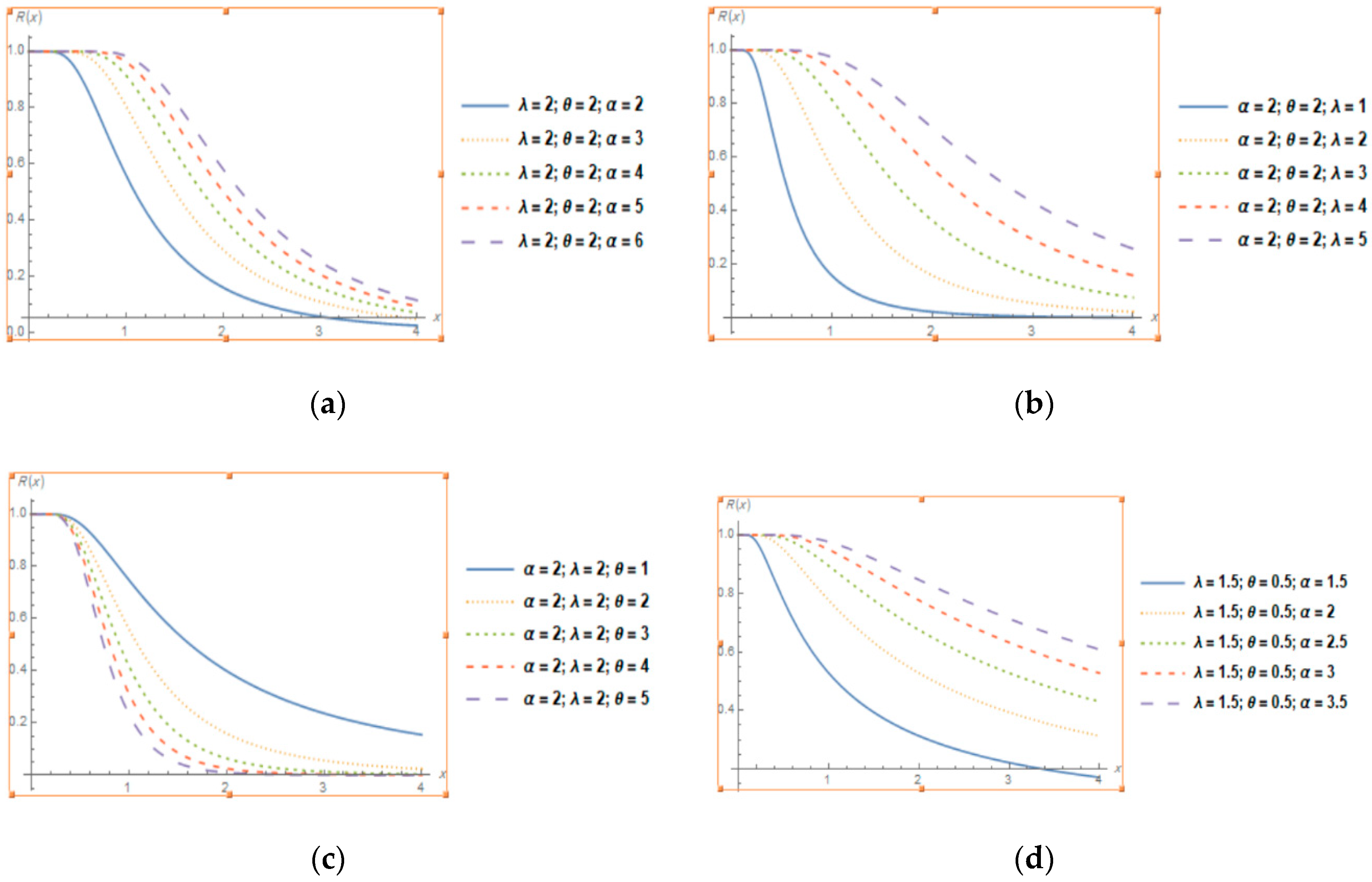
Figure 2 shows that the reliability curves for different values of the parameters for TLGIE distribution is decreasing. Figure 3 shows that the hazard function for different values of the parameters for TLGIE is increasing at first then decreasing in shape i.e., it takes the upside-down bathtub shaped. The lifetime models that present first increase and then decrease shaped failure rates are very useful in survival analysis.

3.4. Hazard Rate Function

It is another characteristic in reliability analysis. It is denoted by h(y). For TLGIE the hazard function is defined as follows
h   (   x   )   =   2   θ   λ   α x 2 exp   ( λ x )   [ 1 exp   ( λ x ) ] 2   θ   1   [ 1     [ 1 exp   ( λ x ) ] 2   θ ] α   1 1     [ 1   [ 1 exp ( λ x ) ] 2   θ ] α ,

3.5. Mode

We consider the density function of TLGIE distribution given in (6) and take the first derivative with respect to x to obtain the mode of Topp-Leone generalized inverted exponential distribution as follows
d f ( x ) d x = f   ( x ) [ 2 x + λ x 2 ( 2 θ 1 ) λ x 2 exp ( λ x ) [ 1 exp ( λ x ) ] 1 + 2 θ ( α 1 ) λ x 2 exp ( λ x ) [ 1 exp ( λ x ) ] 2 θ 1 [ 1 [ 1 exp ( λ x ) ] 2 θ ] 1 ] ,
By putting d f ( x ) d x = 0 , the maxima can be obtained by solving (17) iteratively using numerical methods as Newton- Raphson.
The mode, median, mean, skewness and kurtosis of the TLGIE distribution for various values of α ,   θ and λ shown in Table 1 and Table 2.
From Table 1 and Table 2, we can study the behavior of the TLGIE distribution by changing the parameter values. We can deduce that if α increases, the mode, median and mean are increased but the skewness and kurtosis are decreased. If θ increases, the mode, median and mean are decreased, else the skewness and kurtosis are decrease. If λ increase, the mode, median and mean are decrease but the skewness and kurtosis remain the same. In any values of parameters, we observe that mode < median < mean, this means that the TLGIE distribution is always right skewed and unimodal.

3.6. The Mean Deviation and the Median Deviation

The mean deviation is a measure of dispersion derived by computing the mean of the absolute values of the differences between the observed values of a variable and the mean or median of the variable. Also, it is called average deviation. The mean deviation about the mean is defined by:
D   ( μ ) =   Ε   | x     μ |   =   0 | x μ | f   ( x )   d x   =   0 μ ( x     μ ) f   ( x )   d x   +   μ ( x     μ ) f   ( x )   d x   =   2   μ   F   ( μ )   2 0 μ x   d F   ( x )   =   2   0 μ F   ( x )   d x ,
By substituting from Equation (9) in (18), we obtain the mean deviation about the mean as:
D ( μ ) = 2 k   =   0 j   =   0 ( 1 ) k + j Γ ( α + 1 ) Γ ( 2 θ k + 1 ) Γ ( k + 1 ) Γ ( α k + 1 ) Γ ( j + 1 ) Γ ( 2 θ k j + 1 ) × 0 μ exp ( λ x j ) d x = 2 k   =   0 j   =   0 (     1   ) k   +   j Γ ( α + 1 ) Γ ( 2 θ k + 1 ) Γ ( k + 1 ) Γ ( α k + 1 ) Γ ( j + 1 ) Γ ( 2 θ k j + 1 ) , × ( μ exp ( λ μ j ) λ j Γ ( 0 , λ μ j ) ) , ( λ μ j ) R > 0
where, Γ ( 0 , λ μ j ) is the incomplete gamma function.
Next, the mean deviation about the median is obtained as:
D   (   m   ) =   Ε   |   x     m   |   =   μ     m   +   2   0 m F   (   x   )   d x ,
And for TLGIE, by substituting from Equation (9) in (20), we obtain the median deviation as:
D ( m ) = μ m + 2 k   =   0 j   =   0 ( 1 ) k + j Γ ( α + 1 ) Γ ( 2 θ k + 1 ) Γ ( k + 1 ) Γ ( α k + 1 ) Γ ( j + 1 ) Γ ( 2 θ k j + 1 ) × 0 m exp ( λ x j ) d x = μ m + 2 k   =   0 j   =   0 (     1   ) k   +   j Γ ( α + 1 ) Γ ( 2 θ k + 1 ) Γ ( k + 1 ) Γ ( α k + 1 ) Γ ( j + 1 ) Γ ( 2 θ k j + 1 ) × ( m exp ( λ m j ) λ j Γ ( 0 , λ m j ) ) , ( λ m j ) R > 0
where, Γ ( 0 , λ m j ) was known in (19).

4. Rényi Entropy of TLGIE

In the present section, we provide an important measure, the Rényi entropy. It was introduced by [24]. It is one of the several generalizations of Shannon’s entropy, see [25]. The theory of entropy has been successfully used in a wide diversity of applications such as in information theory, engineering, and physics, see [26]. Entropy is defined in physics via the second law of thermodynamics. Thermodynamic system that is also usually considered to be a measure of the system’s disorder, that is a property of the system’s state, and that varies directly with any reversible change in heat in the system and inversely with the temperature of the system. In this paper, we interest in the statistical mechanics of entropy. The interpretation of entropy in statistical mechanics is the measure of uncertainty, which remains about a system after its observable macroscopic properties, such as temperature, pressure and volume, have been taken into account. The entropy of a probability distribution can be interpreted not only as a measure of uncertainty but also as a measure of information. It has also been used for the characterization of numerous standard probability distributions. For the density function f (x), the Rényi entropy is defined by:
R β   (   x   )   =   1 1 β   L o g   [   J   (   β   )   ]
where
J   (   β   )   =   0 f β   (   x   )   d x ;   β     1
By substituting from Equation (9) in (23), we obtain:
J ( β ) = ( 2   α   θ   λ ) β k   =   0 j   =   0 ( 1 ) k + j ( β ( α 1 ) k ) ( 2 θ ( β + k ) β j ) 0 x 2 β exp ( λ x ( k + β ) ) d x   = ( 2   α   θ   λ ) β Γ ( 2 β 1 ) k   =   0 j   =   0 ( 1 ) k   +   j [ λ   (   k   +   β   ) ] 2   β     1 × ( 1 ) k + j Γ ( β ( α 1 ) + 1 ) Γ ( 2 θ ( β + k ) β + 1 ) Γ ( k + 1 ) Γ ( j + 1 ) Γ ( β ( α 1 ) k + 1 ) Γ ( 2 θ ( β + k ) β j + 1 ) ,
Thus, the Rényi entropy for TLGIE distribution is
R β   (   x   )   =   1 1 β   L o g   [ ( 2   α   θ   λ ) β Γ ( 2 β 1 ) k   =   0 j   =   0 (     1   ) k   +   j [ λ   (   k   +   β   ) ] 2   β     1 × ( 1 ) k + j Γ ( β ( α 1 ) + 1 ) Γ ( 2 θ ( β + k ) β + 1 ) Γ ( k + 1 ) Γ ( j + 1 ) Γ ( β ( α 1 ) k + 1 ) Γ ( 2 θ ( β + k ) β j + 1 ) ]

5. Parameters Estimation

5.1. Maximum Likelihood Estimation

In this section, we derive the maximum likelihood estimates (MLEs) and inference for unknown parameters of Topp-Leone Generalized Inverted Exponential distribution. Let x 1 ,   x 2 ,     ,   x n be a realization of a random sample of size n from TLGIE distribution then the likelihood function is written as follows
L = i = 0 n f ( y i ) ,
and the log-likelihood function is given as follows
  =   log   (   L   ) =   n   log   (   2   α   θ   λ   )     2   i = 1 n log   (   x i )     i = 1 n   λ x i   +   (   2   θ     1   )   i = 1 n   log   (   1     e   λ x i   )   +   (   α     1   )   i = 1 n   log   ( 1     (   1     e   λ x i   )   2   θ ) ,
Differentiating (25) with respect α , θ , λ , respectively, and equating them to 0, we have
n α   +   i = 1 n   log   ( 1     (   1     e   λ x i   )   2   θ   )   =   0 ,
  n θ   +   2   i = 1 n   log   (   1     e   λ x i   )     2   (   α     1   )   i = 1 n (   1     e   λ x i   )   2   θ log   (   1     e   λ x i   ) 1     (   1     e   λ x i   )   2   θ     =   0 ,
  n λ     i = 1 n   1 x i   +   (   2   θ     1   )   i = 1 n x i   1   e   λ x i   1     e   λ x i       2   θ   (   α     1   )   i = 1 n   x i   1   e   λ x i     (   1     e   λ x i   )   2   θ     1 1     (   1     e   λ x i   )   2   θ   =   0 ,
The maximum likelihood estimates of α ,   θ and   λ are obtained iteratively by solving (26), (27), and (28), simultaneously.

5.2. Fisher Information

The approximate variance covariance matrix of the (MLEs) for the parameters of TLGIE distribution with γ _ = ( α , θ , λ ) is obtained by
I n 1 ( γ _ ) = ( var ( α ) cov ( α , θ ) cov ( α , λ ) cov ( θ , α ) var ( θ ) cov ( θ , λ ) cov ( λ , α ) cov ( λ , θ ) var ( λ ) ) I n 1 ( γ _ ) = ( ( 2 log L γ i γ j ) ) γ = γ
The elements of the observed Fisher information matrix, could be found by using the second partial derivatives of the maximum likelihood estimators as follows
2   log   L α 2   =     n α 2   ,
  2   log   L α   θ   =     2   i = 1 n   (   1     e   λ x i   ) 2   θ log   (   1     e   λ x i   ) 1     (   1     e   λ x i   ) 2   θ   ,
2   log   L α   λ   =     2   θ   i = 1 n   e   λ x i   (   1     e   λ x i   ) 2   θ   + 1 x i   ( 1     (   1     e   λ x i   ) 2   θ )     ,
2   log   L θ 2   =     n θ 2   +   4   (   1     α   )   i = 1 n   (   1     e   λ x i   ) 2   θ     log   (   1     e   λ x i   ) 2     ( 1     (   1     e   λ x i   ) 2   θ ) 2     ,
2   log   L θ   λ =     2   (   1     α   ) i = 1 n   e   λ x i   (   1     e   λ x i   ) 2   θ   1 ( 1   +   2   θ   log   (   1     e   λ x i   ) (   1     e   λ x i   ) 2   θ )   x i   ( 1     (   1     e   λ x i   ) 2   θ ) 2     +   2   i = 1 n   e λ x i x i   (   1     e   λ x i   ) ,
2   log   L λ 2   =     n λ 2   +   (   2   θ     1   )   i = 1 n     e   λ x i     x i 2   (   1     e   λ x i   ) 2       + 2   θ   (   α   1   )   i = 1 n   e   λ x i   (   1     e   λ x i   ) 2   θ     1   ψ i   x i 2   ( 1     (   1     e   λ x i   ) 2   θ ) 2     ,
where: ψ i   =   1     (   1     e   λ x i   ) 2   θ   (   2   θ     1   )   e   λ x i     (   1     e   λ x i   ) 1       e   λ x i     (   1     e   λ x i   )   2   θ   1     .

6. Simulation Study

In this section, we discuss some simulations for different sample size to determine the efficiency of MLEs. We can generate a random variable X from TLGIE using Mathematica (V.11.0). We generate samples of size n = 50; 100; 200; 500 and 1000 from TLGIE distribution for some selected combination of parameters. This process is repeated N = 1000 time to calculate mean estimate, means squared error and bias. Obtained results are given in following tables.
From Table 3, we observed that when sample size increases the mean squared error (MSE) and bias (BIAS) decrease. Therefore, the maximum likelihood method works very well to estimate the parameters of TLGIE distribution.

7. Applications

In this section, we provide the application with real data sets to assess the flexibility of TLGIE distribution. The parameters are estimated using maximum likelihood method.
Mathematica (V.11.0) is used for computation. We describe data sets to find the MLEs of the parameters. To assess the fitness of the real data for proposed distribution, we compared the fitness with Topp-Leone Inverted Exponential distribution (TLIE), Topp-Leone Standard Inverted Exponential distribution (TLSIE), Inverted Exponential distribution (IE) and Topp-Leone Generalized Standard Inverted Exponential distribution (TLGSIE). The required numerical evaluations are carried out using the Mathematica (V.11.0) software. In order to compare the four distribution models, we consider the criteria like AIC (Akaike information criterion), CAIC (consistent Akaike information criteria), see: [27], and HQIC (Hannan-Quinn information criterion), see: [28]. The better distribution corresponds to lesser AIC, CAIC and HQIC values.
In the following, we considered three data sets:

7.1. Data Set 1

The first data set that we considered, see [29], represent 40 patients suffering from blood cancer (Leukemia) from one ministry of health hospital in Saudi Arabia. The ordered life time (in years) are given as follows: 0.315, 0.496, 0.616, 1.145, 1.208, 1.263, 1.414, 2.025, 2.036, 2.162, 2.211, 2.370, 2.532, 2.693, 2.805, 2.910, 2.912, 3.192, 3.263, 3.348, 3.348, 3.427, 3.499, 3.534, 3.767, 3.751, 3.858, 3.986, 4.049, 4.244, 4.323, 4.381, 4.392, 4.397, 4.647, 4.753, 4.929, 4.973, 5.074, 4.381.

7.2. Data Set 2

The second data set consists of the number of successive failures for the air conditioning system of each member in a fleet of 13 Boeing 720 jet airplanes, see [30]. The actual data are: 194, 413, 90, 74, 55, 23, 97, 50, 359, 50, 130, 487, 57, 102, 15, 14, 10, 57, 320, 261, 51, 44, 9, 254, 493, 33, 18, 209, 41, 58, 60, 48, 56, 87, 11, 102, 12, 5, 14, 14, 29, 37, 186, 29, 104, 7, 4, 72, 270, 283, 7, 61, 100, 61, 502, 220, 120, 141, 22, 603, 35, 98, 54, 100, 11, 181, 65, 49, 12, 239, 14, 18, 39, 3, 12, 5, 32, 9, 438, 43, 134, 184, 20, 386, 182, 71, 80, 188, 230, 152, 5, 36, 79, 59, 33, 246, 1, 79, 3, 27, 201, 84, 27, 156, 21, 16, 88, 130, 14, 118, 44, 15, 42, 106, 46, 230, 26, 59, 153, 104, 20, 206, 5, 66, 34, 29, 26, 35, 5, 82, 31, 118, 326, 12, 54, 36, 34, 18, 25, 120, 31, 22, 18, 216, 139, 67, 310, 3, 46, 210, 57, 76, 14, 111, 97, 62, 39, 30, 7, 44, 11, 63, 23, 22, 23, 14, 18, 13, 34, 16, 18, 130, 90, 163, 208, 1, 24, 70, 16, 101, 52, 208, 95, 62, 11, 191, 14, 7.

7.3. Data Set 3

This data set consists of the waiting times (in seconds), between 65 successive eruptions of the Kiama Blowhole. These values were recorded with the aid of digital watch on 12 July 1998 by Jim Irish and has been referenced by [31] and [16]. The actual data are: 83, 51, 87, 60, 28, 95, 8, 27, 15, 10, 18, 16, 29, 54, 91, 8, 17, 55, 10, 35, 47, 77,36, 17, 21, 36, 18, 40, 10, 7, 34, 27, 28, 56, 8, 25, 68, 146, 89, 18, 73, 69, 9, 37, 10, 82, 29,8, 60, 61, 61, 18, 169, 25, 8, 26, 11, 83, 11, 42, 17, 14, 9, 12.
In Table 4, Table 5 and Table 6, the values of log-likelihood (LL), AIC, CAIC and HQIC are minimum and favorable of TLGIE distribution than other existing distributions, which indicates that the new model (TLGIE) is better. It is depicted from the results that our proposed model provides better than other sub models. It is be more reliable with these types of data.
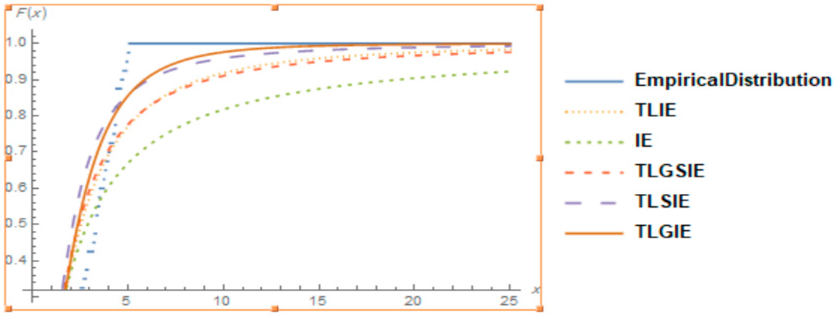
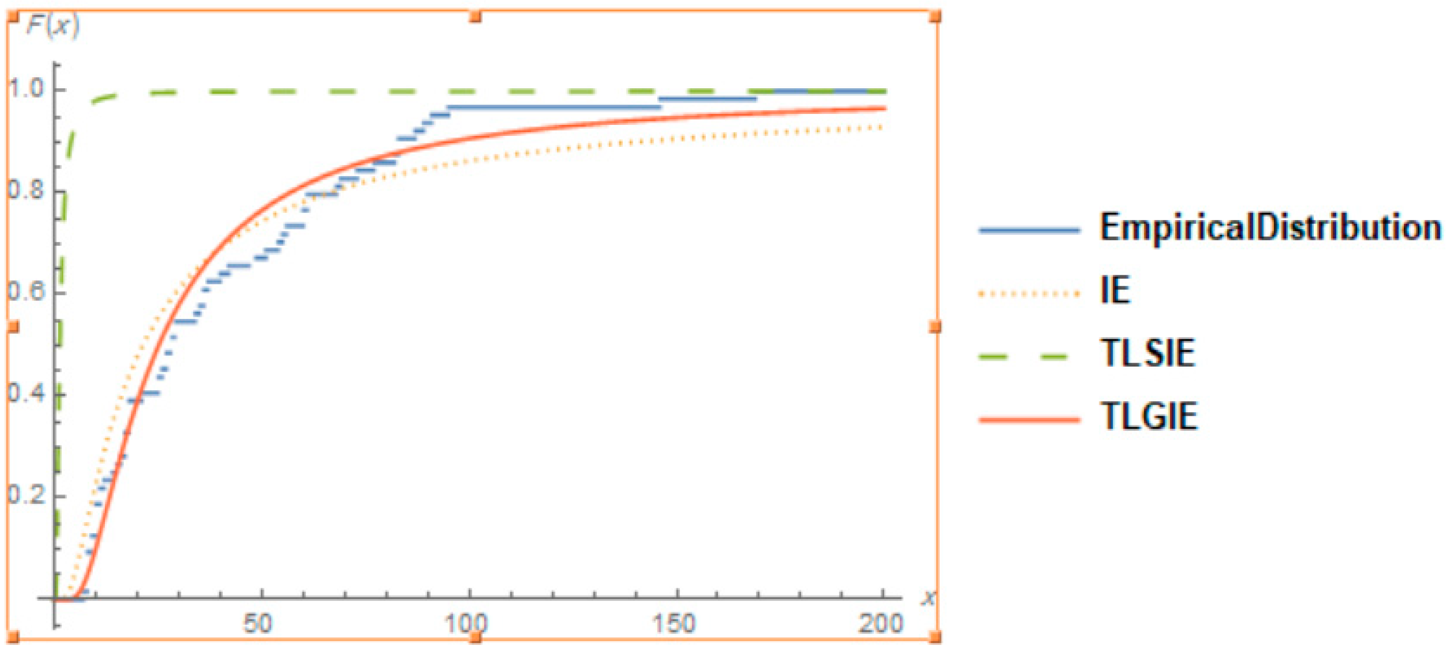
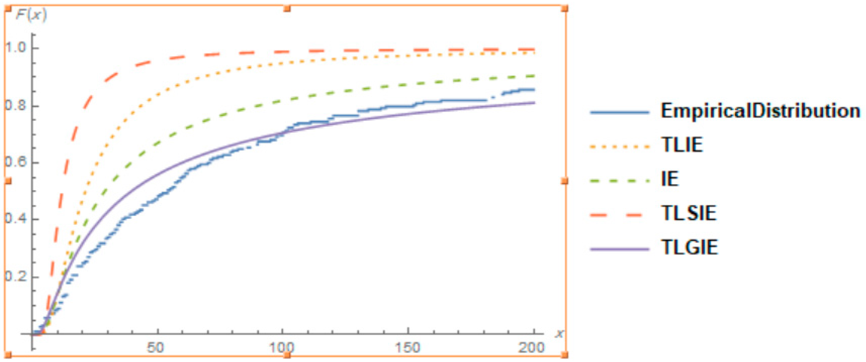
It is also clear from Figure 4, Figure 5 and Figure 6, that the TLGIE distribution provides the best fit as compare to TLIE, TLSIE, IE and TLGSIE for given three data sets. So, the TLGIE model could be chosen as the best model.

8. Conclusions

We derived a three parameter Topp-Leone generalized inverted exponential distribution. Some of desirable properties are computed. The parameters are estimated by method of maximum likelihood. Performance of MLE’s are tested through simulation study. Finally, three real data applications are analyzed to assess the flexibility of new model over existing distribution. It is significantly observed that the proposed model provides better result than derived models.

Author Contributions

The two authors contributed in methodology and investigation. They have read and agreed to the published version of the manuscript. All authors have read and agreed to the published version of the manuscript.

Funding

This work was funded by the University of Jeddah, Saudi Arabia under grant No. (UJ-02-088-DR). The authors, therefore, acknowledge with thanks the University technical and financial support.

Acknowledgments

The authors would like to thank the two reviewers for careful reading and for their valuable comments that improved the research.

Conflicts of Interest

The authors declare no conflict of interest.

Abbreviations

TLGIETopp-Leon Generalized Inverted Exponential
GIEGeneralized Inverted Exponential
TLTopp-Leone
cdfcumulative distribution function
pdfprobability distribution function
TLIETopp-Leone Inverted Exponential
TLSIETopp-Leone Standard Inverted Exponential
IEInverted Exponential
TLGSIETopp-Leone Generalized Standard Inverted Exponential
EGIEGeneralized Inverted Exponential
Ε r ( 1 ) the integration exponential function
CVcoefficient of variation
CScoefficient of skewness
CKcoefficient of kurtosis
MLEmaximum likelihood estimate
MSEmean squared error
AICAkaike information criterion
CAICconsistent Akaike information criterion
HQICHannan-Quinn information criterion
MLEsthe maximum likelihood estimates
LThe likelihood function
the log-likelihood function
BIASbias
LLlog-likelihood
g ( x ) pdf of GIE
G ( x ) Cdf of GIE
F T L G ( x ) Cdf of TL distribution
f T L G ( x ) Pdf of TL distribution
R (x)The reliability or survival function
h(y)The hazard function
D ( μ ) The mean deviation
D ( m ) The median deviation

References

  1. Abouammoh, A.M.; Alshingiti, A.M. Reliability estimation of generalized inverted exponential distribution. J. Stat. Comput. Simul. 2009, 79, 1301–1315. [Google Scholar] [CrossRef]
  2. Zografos, K.; Balakrishnan, N. On families of beta- and generalized gamma- generated distributions and associated inference. Stat. Methodol. 2009, 6, 344–362. [Google Scholar] [CrossRef]
  3. Cordeiro, G.M.; de Castro, M. A new family of generalized distributions. J. Stat. Comput. Simul. 2011, 81, 883–898. [Google Scholar] [CrossRef]
  4. Alexander, C.; Cordeiro, G.M.; Ortega, E.M.M.; Sarabia, J.M. Generalized Beta-generated distributions. Comput. Stat. Data Anal. 2012, 56, 1880–1897. [Google Scholar] [CrossRef]
  5. Bourguignon, M.; Silva, R.B.; Cordeiro, G.M. The Weibull-G family of probability distributions. J. Data Sci. 2014, 12, 53–68. [Google Scholar]
  6. Alizadeh, M.; Emadiz, M.; Doostparast, M.; Cordeiro, G.M.; Ortega, E.M.M.; Pescim, R.R. A new family of distributions: The Kumaraswamy odd log-logistic, properties and applications. Hacet. J. Math. Stat. 2015, 44, 1491–1512. [Google Scholar] [CrossRef]
  7. Alizadeh, M.; Altun, E.; Cordeiro, G.M.; Rasekhi, M. The odd power Cauchy family of distributions: Properties, regression models and applications. J. Stat. Comput. Simul. 2018, 88, 785–805. [Google Scholar] [CrossRef]
  8. Topp, C.W.; Leone, F.C. A family of J-shaped frequency functions. J. Amer. Stat. Assoc. 1955, 50, 209–219. [Google Scholar] [CrossRef]
  9. Nadarajah, S.; Kotz, S. Moments of some J-shaped distributions. J. Appl. Stat. 2003, 30, 311–317. [Google Scholar] [CrossRef]
  10. Ghitany, M.E.; Kotz, S.; Xie, M. On some reliability measures and their stochastic orderings for the Topp- Leone distribution. J. Appl. Stat. 2005, 32, 715–722. [Google Scholar] [CrossRef]
  11. Kotz, S.; Seier, E. Kurtosis of the Topp-Leone distributions. Interstat 2007, 1–15. [Google Scholar]
  12. Vicaria, D.; Dorpb, J.R.V.; Kotzb, S. Two-sided generalized Topp and Leone (TS-GTL) distributions. J. Appl. Stat. 2008, 35, 1115–1129. [Google Scholar] [CrossRef]
  13. Al-Zahrani, B. Goodness-of-fit for the Topp-Leone distribution with unknown parameters. Appl. Math. Sci. 2012, 6, 6355–6363. [Google Scholar]
  14. Sangsanit, Y.; Bodhisuwan, W. The Topp-Leone generator of distributions: Properties and inferences. Songklanakarin J. Sci. Technol. 2016, 38, 537–548. [Google Scholar]
  15. Al-Shomrani, A.; Arif, O.; Shawky, A.; Hanif, S.; Shahbaz, M.Q. Topp leone family of distributions: Some properties and application. Pak. J. Stat. Oper. Res. 2016, 2, 443–451. [Google Scholar] [CrossRef] [Green Version]
  16. Abbas, S.; Taqi, S.A.; Mustafa, F.; Murtaza, M.; Shahbaz, M.Q. Topp-Leone Inverse Weibull distribution: Theory and Application. Eur. J. Pure Appl. Math. 2017, 10, 1005–1022. [Google Scholar]
  17. Elgarhy, M.; Nasir, M.A.; Jamal, F.; Ozel, G. The type II Topp-Leone generated family of distributions: Properties and applications. J. Stat. Manag. Syst. 2018, 21, 1529–1551. [Google Scholar] [CrossRef]
  18. Arshad, M.; Jamal, Q.A. Statistical Inference for Topp–Leone-generated Family of Distributions Based on Records. J. Stat. Theory Appl. 2019, 18, 65–78. [Google Scholar]
  19. Ibrahim, S.; Doguwa, I.S.; Audu, I.; Muhammad, H.J. On the Topp Leone Exponentiated-G Family of Distributions: Properties and Applications. Asian J. Probab. Stat. 2020, 7, 1–15. [Google Scholar] [CrossRef] [Green Version]
  20. Ibrahim, S.; Doguwa, I.S.; Audu, I.; Muhammad, H.J. On the Flexibility of Topp Leone Exponentiated Inverse Exponential Distribution. Int. J. Data Sci. Anal. 2020, 6, 83–89. [Google Scholar] [CrossRef]
  21. Bantan, R.A.; Jamal, F.; Chesneau, C.; Elgarhy, M. Type II Power Topp-Leone Generated Family of Distributions with Statistical Inference and Applications. Symmetry 2020, 12, 75. [Google Scholar] [CrossRef] [Green Version]
  22. Al-Marzouki, S.; Jamal, F.; Chesneau, C.; Elgarhy, M. Type II Topp Leone Power Lomax Distribution with Applications. Mathematics 2020, 8, 4. [Google Scholar] [CrossRef] [Green Version]
  23. Prudnikov, A.P.; Brychkov, Y.A.; Marichev, O.I. Integrals and Series; Gordon and Breach Science Publishers: New York, NY, USA, 1986; Volume 3. [Google Scholar]
  24. Rényi, A. On the dimension and entropy of probability distributions. Acta Math. Hung. 1959, 10, 193–215. [Google Scholar] [CrossRef]
  25. Shannon, C.E. A note on the concept of entropy. Bell Syst. Tech. J. 1948, 27, 379–423. [Google Scholar] [CrossRef] [Green Version]
  26. Song, K.S. Rényi information, loglikelihood and an intrinsic distribution measure. J. Stat. Plan. Inference 2001, 93, 51–69. [Google Scholar] [CrossRef]
  27. Hurvich, C.M.; Tsai, C.L. A corrected Akaike information criterion for vector autoregressive model selection. J. Time Ser. Anal. 1994, 14, 271–279. [Google Scholar] [CrossRef]
  28. Hannan, E.J.; Quinn, B.G. The determination of the order of an autoregression. J. R. Stat. Soc. Ser. B. 1979, 41, 190–195. [Google Scholar] [CrossRef]
  29. Atallah, M.; Mahmoud, M.; Al-Zahrani, B. A new test for exponentiality versus nbumgf life distributions based on laplace transform. Qual. Reliab. Eng. Int. 2014, 30, 1353–1359. [Google Scholar] [CrossRef]
  30. Proschan, F. Theoretical explanation of observed decreasing failure rate. Technometrics 1963, 5, 375–383. [Google Scholar] [CrossRef]
  31. Pinho, L.G.; Cordeiro, G.M.; Nobre, J.S. The Harris extended exponential distribution. Commun. Stat. Theory Methods 2015, 44, 3486–3502. [Google Scholar] [CrossRef]
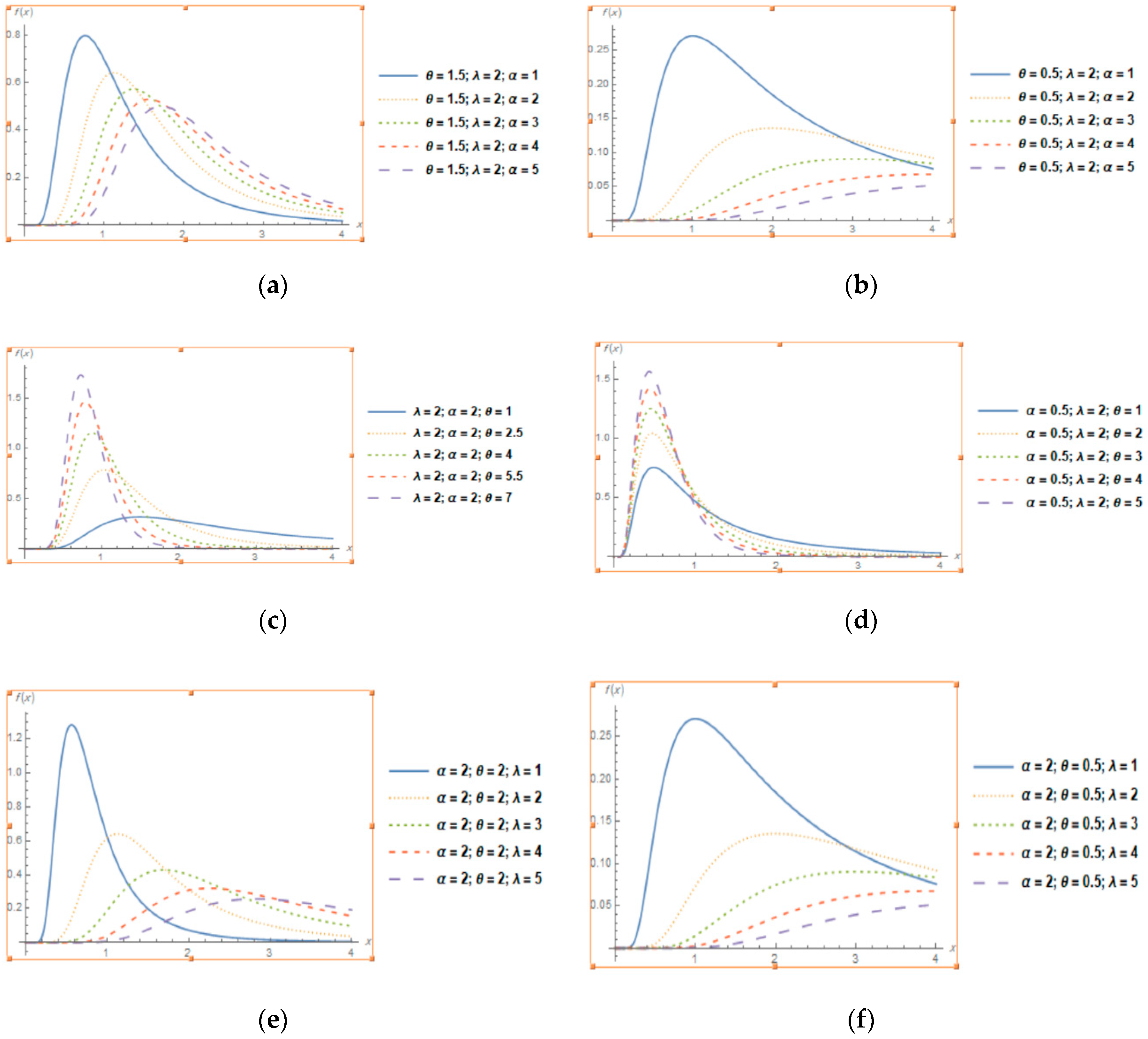
Figure 1. Plots of the pdf of TLGIE distribution for selected values of the parameters when (a,b) α increases, (c,d) θ increases and (e,f) λ increases.
Entropy 22 01144 g001
Figure 2. Plots of the reliability function of TLGIE distribution for selected values of the parameters when (a,d) α increases, (b) λ increases and (c) θ increases.
Entropy 22 01144 g002
Figure 3. Plots of the Hazard Function of TLGIE distribution for selected values of the parameters when (a,b) α increases, (c) λ increases and (d) θ increases.
Entropy 22 01144 g003aEntropy 22 01144 g003b
Figure 4. Plots of the Goodness of Fit of TLGIE distribution using data set 1.
Entropy 22 01144 g004
Figure 5. Plots of the Goodness of Fit of TLGIE distribution using data set 2.
Entropy 22 01144 g005
Figure 6. Plots of the Goodness of Fit of TLGIE distribution using data set 3.
Entropy 22 01144 g006
Table 1. The mode, median, mean, skewness and kurtosis of the TLGIE distribution for λ = 2 , θ = { 1 , 1.5 , 2 }   a n d   α = { 1 , 1.5 , 2 } .
α ModeMedianMeanSkewnessKurtosis
θ = 1 , λ = 2
10.8838571.628732.772590.3295011.01815
1.51.210142.133833.535760.3234350.998774
21.493852.566964.185990.3200470.988074
θ = 1.5 , λ = 2
10.8131071.267081.726090.2668250.783853
1.51.061671.580272.102950.2601120.764511
21.263681.833262.406670.256540.754304
θ = 2 , λ = 2
10.7639371.088021.359190.2301640.66022
1.50.968121.321121.61770.2237270.642568
21.127481.503171.819710.2204720.63372
Table 2. The mode, median, mean, skewness and kurtosis of the TLGIE distribution for θ = 2 , λ = { 1.5 , 2 , 2.5 }   a n d   α = { 1 , 1.5 , 2.5 } .
α ModeMedianMeanSkewnessKurtosis
θ = 2 , λ = 1.5
10.5729530.8160161.019390.2301640.66022
1.50.726090.9908431.213280.2237270.642568
2.50.9447911.240771.490670.2185230.628463
θ = 2 , λ = 2
10.7639371.088021.359190.2301640.66022
1.50.968121.321121.61770.2237270.642568
2.51.259721.654361.987570.2185230.628463
θ = 2 , λ = 2.5
10.9549221.360031.698990.2301640.66022
1.51.210151.651412.022132.022130.642568
2.51.574652.067942.484460.2185230.628463
Table 3. Estimated Mean, MSEs and BIAS of TLGIE distribution.
True Values : α = 1 θ = 1 λ = 1
n α θ λ
50MLE1.649441.36561.63393
MSE2.542940.9352212.53382
BIAS0.6494390.3655950.633934
100MLE1.537641.20621.481
MSE2.046450.3121221.76203
BIAS0.5376360.20620.481003
200MLE1.489961.098781.28113
MSE1.728860.09874320.980768
BIAS0.4899580.09877820.281133
500MLE1.284381.037961.11058
MSE0.8889280.02821870.34375
BIAS0.2843840.03795920.110576
1000MLE1.128721.023041.0703
MSE0.3595090.01256710.168361
BIAS0.128720.02304310.0703043
Table 4. Parameters Estimation for Various Distributions depending on data set 1.
ModelParametersLLAICCAICHQIC
α θ λ
TLGIE0.4186852.190257.26267−82.2875170.575171.242172.407
TLIE0.589171 4.55247−85.5231175.046175.37176.267
TLSIE4.55482 −90.3942182.788182.894183.399
IE 2.00825−91.1589184.318184.423184.929
TLGSIE3.21550.755551 −88.1251180.25180.575181.472
Table 5. Parameters Estimation for Various Distributions depending on data set 2.
ModelParametersLLAICCAICHQIC
α θ λ
TLGIE8.846530.3613131.11353−1065.132136.252136.382140.18
TLIE1.20401 22.9514−1164.412332.832332.892335.45
TLSIE106.161 −1379.432762.862762.922765.4
IE 19.9992−1082.512167.012167.032168.32
Table 6. Parameters Estimation for Various Distributions depending on data set 3.
ModelParametersLLAICCAICHQIC
α θ λ
TLGIE2.068610.7744814.7643−295.07596.14596.54598.691
TLSIE283.888 −304.914611.828611.893612.679
IE 20.4134−299.175600.351600.415601.201