Decision Tree Integration Using Dynamic Regions of Competence


Abstract
1. Introduction
- A proposal of a new partitioning of the feature space whose split is determined by the decision bonduaries of each decision tree node which is a base classification model.
- The proposal of a new weighted majority voting rule algorithm dedicated to the fusion of decision tree models.
- An experimental setup to compare the proposed method with other MCS approaches using different performance measures.
2. Related Works
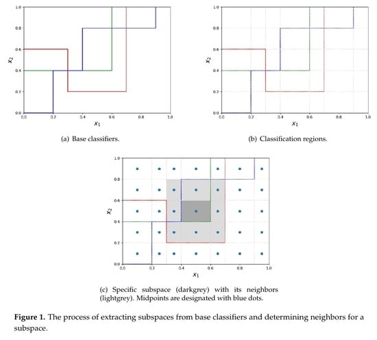
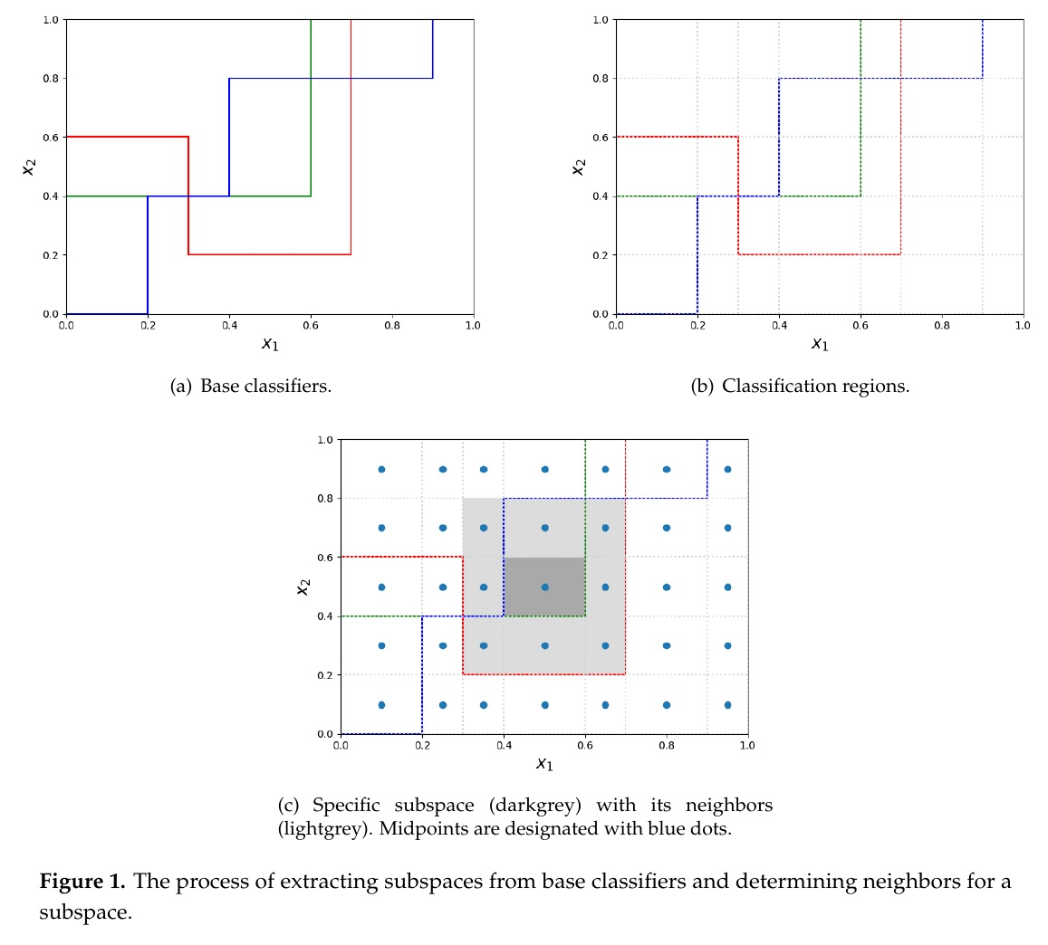
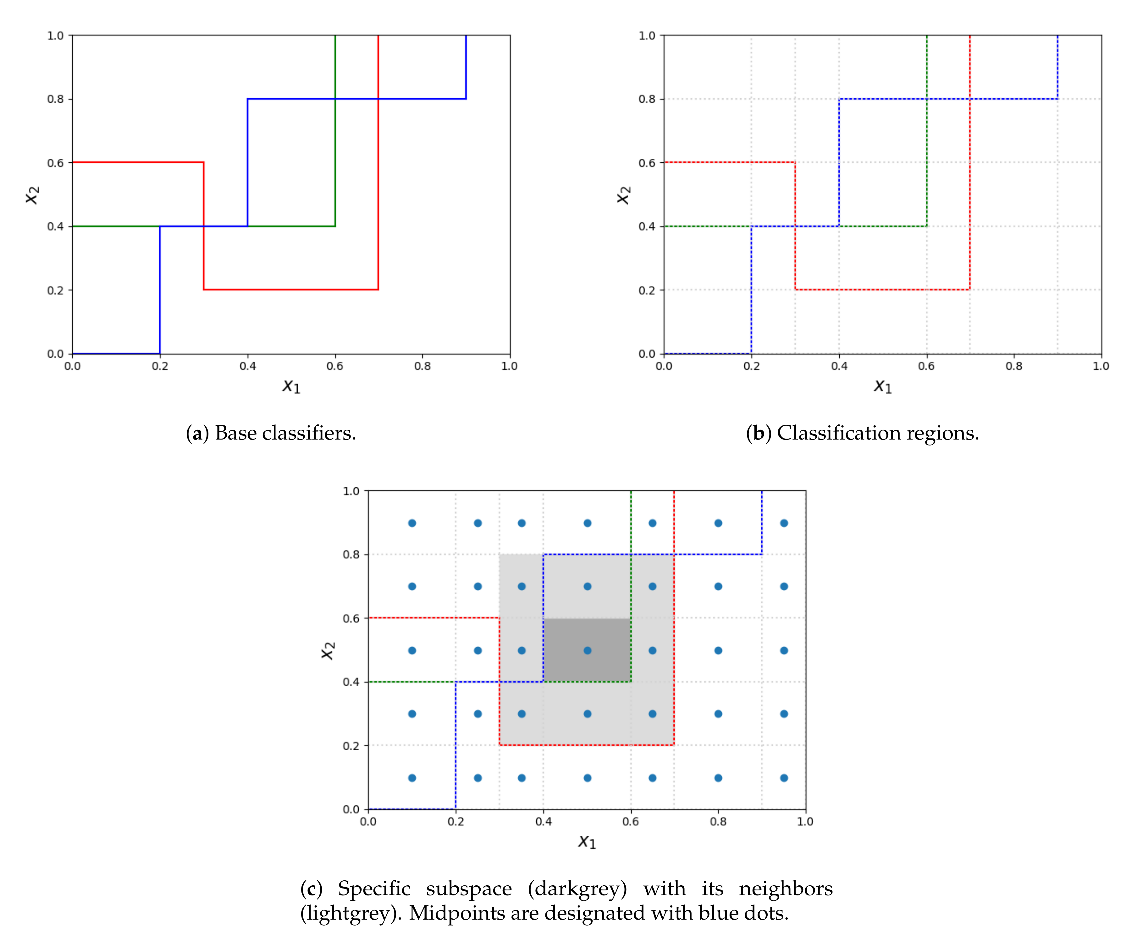
3. Proposed Method
- Their area is maximal.
- Every point they span is labeled with the same label by every single classifier (labels can differ across different classifiers). In other words regions span over the area of objects equally labelled by the classifier points.
| Algorithm 1: Classification algorithm using dynamic regions of competence obtained from decision trees. |
|
4. Experimental Setup
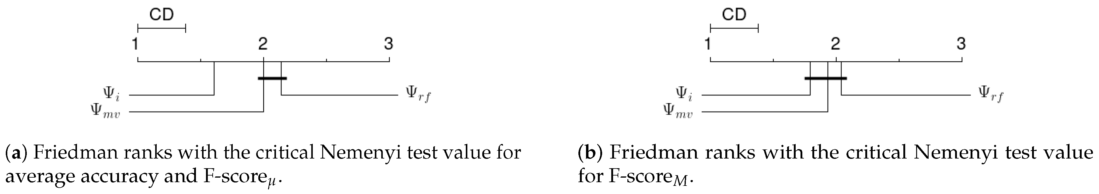
5. Results
6. Discussion
7. Conclusions
Author Contributions
Funding
Conflicts of Interest
Abbreviations
| MV | Majority Voting |
| RF | Random Forest |
| SVM | Support Vector Machine |
References
- Sagi, O.; Rokach, L. Ensemble learning: A survey. Wiley Interdiscip. Rev.-Data Mining Knowl. Discov. 2018, 8, e1249. [Google Scholar] [CrossRef]
- Alpaydin, E. Introduction to Machine Learning; MIT Press: Cambridge, MA, USA, 2020. [Google Scholar]
- Andrysiak, T. Machine learning techniques applied to data analysis and anomaly detection in ECG signals. Appl. Artif. Intell. 2016, 30, 610–634. [Google Scholar] [CrossRef]
- Burduk, A.; Grzybowska, K.; Safonyk, A. The Use of a Hybrid Model of the Expert System for Assessing the Potentiality Manufacturing the Assumed Quantity of Wire Harnesses. LogForum 2019, 15, 459–473. [Google Scholar] [CrossRef]
- Dutta, V.; Choraś, M.; Pawlicki, M.; Kozik, R. A Deep Learning Ensemble for Network Anomaly and Cyber-Attack Detection. Sensors 2020, 20, 4583. [Google Scholar] [CrossRef]
- Heda, P.; Rojek, I.; Burduk, R. Dynamic Ensemble Selection–Application to Classification of Cutting Tools. In International Conference on Computer Information Systems and Industrial Management; Springer: Berlin/Heidelberg, Germany, 2020; pp. 345–354. [Google Scholar]
- Xiao, J. SVM and KNN ensemble learning for traffic incident detection. Physica A 2019, 517, 29–35. [Google Scholar] [CrossRef]
- Rokach, L. Decomposition methodology for classification tasks: A meta decomposer framework. Pattern Anal. Appl. 2006, 9, 257–271. [Google Scholar] [CrossRef]
- Burduk, R. Classifier fusion with interval-valued weights. Pattern Recognit. Lett. 2013, 34, 1623–1629. [Google Scholar] [CrossRef]
- Mao, S.; Jiao, L.; Xiong, L.; Gou, S.; Chen, B.; Yeung, S.K. Weighted classifier ensemble based on quadratic form. Pattern Recognit. 2015, 48, 1688–1706. [Google Scholar] [CrossRef]
- Woźniak, M.; Graña, M.; Corchado, E. A survey of multiple classifier systems as hybrid systems. Inf. Fusion 2014, 16, 3–17. [Google Scholar] [CrossRef]
- Aguilera, J.; González, L.C.; Montes-y Gómez, M.; Rosso, P. A new weighted k-nearest neighbor algorithm based on newton’s gravitational force. In Iberoamerican Congress on Pattern Recognition; Montes-y Gómez, M., Ed.; Springer: Berlin/Heidelberg, Germany, 2018; pp. 305–313. [Google Scholar]
- Ksieniewicz, P.; Burduk, R. Clustering and Weighted Scoring in Geometric Space Support Vector Machine Ensemble for Highly Imbalanced Data Classification. In International Conference on Computational Science; Springer: Berlin/Heidelberg, Germany, 2020; pp. 128–140. [Google Scholar]
- Geler, Z.; Kurbalija, V.; Ivanović, M.; Radovanović, M. Weighted kNN and constrained elastic distances for time-series classification. Expert Syst. Appl. 2020, 113829. [Google Scholar]
- Guggari, S.; Kadappa, V.; Umadevi, V. Non-sequential partitioning approaches to decision tree classifier. Future Computing Inform. J. 2018, 3, 275–285. [Google Scholar] [CrossRef]
- Ho, T.K. The random subspace method for constructing decision forests. IEEE Trans. Pattern Anal. Mach. Intell. 1998, 20, 832–844. [Google Scholar]
- Kuncheva, L.I. Clustering-and-selection model for classifier combination. In KES’2000. Fourth International Conference on Knowledge-Based Intelligent Engineering Systems and Allied Technologies. Proceedings (Cat. No. 00TH8516); IEEE: Piscataway, NJ, USA, 2000; Volume 1, pp. 185–188. [Google Scholar]
- Jackowski, K.; Wozniak, M. Algorithm of designing compound recognition system on the basis of combining classifiers with simultaneous splitting feature space into competence areas. Pattern Anal. Appl. 2009, 12, 415. [Google Scholar] [CrossRef]
- Lopez-Garcia, P.; Masegosa, A.D.; Osaba, E.; Onieva, E.; Perallos, A. Ensemble classification for imbalanced data based on feature space partitioning and hybrid metaheuristics. Appl. Intell. 2019, 49, 2807–2822. [Google Scholar] [CrossRef]
- Pujol, O.; Masip, D. Geometry-Based Ensembles: Toward a Structural Characterization of the Classification Boundary. IEEE Trans. Pattern Anal. Mach. Intell. 2009, 31, 1140–1146. [Google Scholar] [CrossRef]
- Burduk, R. Integration Base Classifiers in Geometry Space by Harmonic Mean. In Artificial Intelligence and Soft Computing; Rutkowski, L., Scherer, R., Korytkowski, M., Pedrycz, W., Tadeusiewicz, R., Zurada, J.M., Eds.; Springer: Berlin/Heidelberg, Germany, 2018; pp. 585–592. [Google Scholar]
- Burduk, R.; Biedrzycki, J. Integration and Selection of Linear SVM Classifiers in Geometric Space. J. Univers. Comput. Sci. 2019, 25, 718–730. [Google Scholar]
- Biedrzycki, J.; Burduk, R. Integration of decision trees using distance to centroid and to decision boundary. J. Univers. Comput. Sci. 2020, 26, 720–733. [Google Scholar]
- Biedrzycki, J.; Burduk, R. Weighted scoring in geometric space for decision tree ensemble. IEEE Access 2020, 8, 82100–82107. [Google Scholar] [CrossRef]
- Polianskii, V.; Pokorny, F.T. Voronoi Boundary Classification: A High-Dimensional Geometric Approach via Weighted M onte C arlo Integration. In International Conference on Machine Learning; Omnipress: Madison, WI, USA, 2019; pp. 5162–5170. [Google Scholar]
- Biau, G.; Devroye, L. Lectures on the Nearest Neighbor Method; Springer: Berlin/Heidelberg, Germany, 2015. [Google Scholar]
- Kushilevitz, E.; Ostrovsky, R.; Rabani, Y. Efficient search for approximate nearest neighbor in high dimensional spaces. SIAM J. Comput. 2000, 30, 457–474. [Google Scholar] [CrossRef]
- Kheradpisheh, S.R.; Behjati-Ardakani, F.; Ebrahimpour, R. Combining classifiers using nearest decision prototypes. Appl. Soft. Comput. 2013, 13, 4570–4578. [Google Scholar] [CrossRef]
- Gou, J.; Zhan, Y.; Rao, Y.; Shen, X.; Wang, X.; He, W. Improved pseudo nearest neighbor classification. Knowl.-Based Syst. 2014, 70, 361–375. [Google Scholar] [CrossRef]
- Rokach, L. Decision forest: Twenty years of research. Inf. Fusion 2016, 27, 111–125. [Google Scholar] [CrossRef]
- Quinlan, J.R. Induction of Decision Trees. Mach. Learn. 1986, 1, 81–106. [Google Scholar] [CrossRef]
- Tan, P.N.; Steinbach, M.M.; Kumar, V. Introduction to Data Mining; Addison-Wesley: Boston, MA, USA, 2005. [Google Scholar]
- Ponti, M.P. Combining Classifiers: From the Creation of Ensembles to the Decision Fusion. In Proceedings of the 2011 24th SIBGRAPI Conference on Graphics, Patterns, and Images Tutorials, Alagoas, Brazil, 28–30 August 2011; pp. 1–10. [Google Scholar]
- Kim, E.; Ko, J. Dynamic Classifier Integration Method. In Multiple Classifier Systems; Oza, N.C., Polikar, R., Kittler, J., Roli, F., Eds.; Springer: Berlin/Heidelberg, Germany, 2005; pp. 97–107. [Google Scholar]
- Sultan Zia, M.; Hussain, M.; Arfan Jaffar, M. A novel spontaneous facial expression recognition using dynamically weighted majority voting based ensemble classifier. Multimed. Tools Appl. 2018, 77, 25537–25567. [Google Scholar] [CrossRef]
- Hajdu, A.; Hajdu, L.; Jonas, A.; Kovacs, L.; Toman, H. Generalizing the majority voting scheme to spatially constrained voting. IEEE Trans. Image Process. 2013, 22, 4182–4194. [Google Scholar] [CrossRef] [PubMed]
- Rahman, A.F.R.; Alam, H.; Fairhurst, M.C. Multiple Classifier Combination for Character Recognition: Revisiting the Majority Voting System and Its Variations. In Document Analysis Systems V; Lopresti, D., Hu, J., Kashi, R., Eds.; Springer: Berlin/Heidelberg, Germany, 2002; pp. 167–178. [Google Scholar]
- Breiman, L. Random Forests. Mach. Learn. 2001, 45, 5–32. [Google Scholar] [CrossRef]
- Fernández-Delgado, M.; Cernadas, E.; Barro, S.; Amorim, D. Do we need hundreds of classifiers to solve real world classification problems? J. Mach. Learn. Res. 2014, 15, 3133–3181. [Google Scholar]
- Chen, T.; Guestrin, C. XGBoost: A Scalable Tree Boosting System. In Proceedings of the 22nd ACM SIGKDD International Conference on Knowledge Discovery and Data Mining; Association for Computing Machinery: New York, NY, USA, 2016; pp. 785–794. [Google Scholar]
- Taieb, S.B.; Hyndman, R.J. A gradient boosting approach to the Kaggle load forecasting competition. Int. J. Forecast. 2014, 30, 382–394. [Google Scholar] [CrossRef]
- Sheridan, R.P.; Wang, W.M.; Liaw, A.; Ma, J.; Gifford, E.M. Extreme Gradient Boosting as a Method for Quantitative Structure-Activity Relationships. J. Chem Inf. Model. 2016, 56, 2353–2360. [Google Scholar] [CrossRef]
- Friedman, J.H. Greedy function approximation: A gradient boosting machine. Ann. Stat. 2001, 29, 1189–1232. [Google Scholar] [CrossRef]
- Ke, G.; Meng, Q.; Finley, T.; Wang, T.; Chen, W.; Ma, W.; Ye, Q.; Liu, T.Y. LightGBM: A highly efficient gradient boosting decision tree. In NIPS’17 Proceedings of the 31st International Conference on Neural Information Processing Systems; Curran Associates Inc.: Red Hook, NY, USA, 2017; pp. 3149–3157. [Google Scholar]
- Chawla, N.V.; Hall, L.O.; Bowyer, K.W.; Kegelmeyer, W.P. Learning Ensembles from Bites: A Scalable and Accurate Approach. J. Mach. Learn. Res. 2004, 5, 421–451. [Google Scholar]
- Meng, X.; Bradley, J.; Yavuz, B.; Sparks, E.; Venkataraman, S.; Liu, D.; Freeman, J.; Tsai, D.; Amde, M.; Owen, S.; et al. MLlib: Machine Learning in Apache Spark. J. Mach. Learn. Res. 2015, 17, 1235–1241. [Google Scholar]
- Oliphant, T. NumPy: A guide to NumPy; Trelgol Publishing: Spanish Fork, UT, USA, 2006. [Google Scholar]
- Jones, E.; Oliphant, T.; Peterson, P. SciPy: Open Source Scientific Tools for Python. Available online: https://www.mendeley.com/catalogue/cc1d80ce-06d6-3fc5-a6cf-323eaa234d84/ (accessed on 20 September 2020).
- McKinney, W. Data Structures for Statistical Computing in Python. In Proceedings of the 9th Python in Science Conference, Austin, TX, USA, 28 June–3 July 2020; van der Walt, S., Millman, J., Eds.; pp. 56–61. [Google Scholar] [CrossRef]
- Hunter, J.D. Matplotlib: A 2D graphics environment. Comput. Sci. Eng. 2007, 9, 90–95. [Google Scholar] [CrossRef]
- Dua, D.; Graff, C. UCI Machine Learning Repository. 2017. Available online: https://ergodicity.net/2013/07/ (accessed on 20 September 2020).
- Alcalá-Fdez, J.; Fernández, A.; Luengo, J.; Derrac, J.; García, S.; Sánchez, L.; Herrera, F. Keel data-mining software tool: Data set repository, integration of algorithms and experimental analysis framework. J. Mult.-Valued Log. Soft Comput. 2011, 17. [Google Scholar]
- Ortigosa-Hernández, J.; Inza, I.; Lozano, J.A. Measuring the class-imbalance extent of multi-class problems. Pattern Recognit. Lett. 2017, 98, 32–38. [Google Scholar] [CrossRef]
- Sokolova, M.; Lapalme, G. A systematic analysis of performance measures for classification tasks. Inform. Process Manag. 2009, 45, 427–437. [Google Scholar] [CrossRef]
- Van Asch, V. Macro- and Micro-Averaged Evaluation Measures; Basic Draft; CLiPS: Antwerpen, Belgium, 2013; Volume 49. [Google Scholar]


| Dataset | #inst | #f | Imb |
|---|---|---|---|
| Indoor Channel Measurements (aa) | 7840 | 5 | 208.0 |
| Appendicitis (ap) | 106 | 7 | 4.0 |
| Banana (ba) | 5300 | 2 | 5.9 |
| QSAR biodegradation (bi) | 1055 | 41 | 2.0 |
| Liver Disorders (BUPA) (bu) | 345 | 6 | 1.4 |
| Cryotherapy (c) | 90 | 7 | 1.1 |
| Banknote authentication (d) | 1372 | 5 | 1.2 |
| Ecoli (e) | 336 | 7 | 71.5 |
| Haberman’s Survival (h) | 306 | 3 | 2.8 |
| Ionosphere (io) | 351 | 34 | 1.8 |
| Iris plants (ir) | 150 | 4 | 1.0 |
| Magic (ma) | 19,020 | 10 | 1.0 |
| Ultrasonic flowmeter diagnostics (me) | 540 | 173 | 1.4 |
| Phoneme (ph) | 5404 | 5 | 2.4 |
| Pima (pi) | 768 | 8 | 1.9 |
| Climate model simulation crashes (po) | 540 | 18 | 10.7 |
| Ring (r) | 7400 | 20 | 1.0 |
| Spambase (sb) | 4597 | 57 | 1.5 |
| Seismic-bumps (se) | 2584 | 19 | 14.2 |
| Texture (te) | 5500 | 40 | 1.0 |
| Thyroid (th) | 7200 | 21 | 1.0 |
| Titanic (ti) | 2201 | 3 | 2.1 |
| Twonorm (tw) | 7400 | 20 | 1.0 |
| Breast Cancer (Diagnostic) (wd) | 569 | 30 | 1.7 |
| Breast Cancer (Original) (wi) | 699 | 9 | 1.9 |
| Wine quality – red (wr) | 1599 | 11 | 68.1 |
| Wine quality – white (ww) | 4898 | 11 | 439.6 |
| Yeast (y) | 1484 | 8 | 92.6 |
| Average Accuracy | F-Scoreμ | F-ScoreM | |||||||
|---|---|---|---|---|---|---|---|---|---|
| Dataset | |||||||||
| aa | 0.917 | 0.918 | 0.919 | 0.469 | 0.474 | 0.477 | 0.196 | 0.192 | 0.176 |
| ap | 0.853 | 0.812 | 0.863 | 0.853 | 0.812 | 0.863 | 0.676 | 0.559 | 0.692 |
| ba | 0.789 | 0.808 | 0.815 | 0.683 | 0.712 | 0.722 | 0.483 | 0.493 | 0.502 |
| bi | 0.736 | 0.736 | 0.702 | 0.736 | 0.736 | 0.702 | 0.717 | 0.717 | 0.561 |
| bu | 0.579 | 0.527 | 0.536 | 0.579 | 0.527 | 0.536 | 0.563 | 0.520 | 0.512 |
| c | 0.762 | 0.867 | 0.684 | 0.762 | 0.867 | 0.684 | 0.773 | 0.870 | 0.698 |
| d | 0.935 | 0.935 | 0.938 | 0.935 | 0.935 | 0.938 | 0.934 | 0.934 | 0.936 |
| e | 0.825 | 0.827 | 0.825 | 0.414 | 0.423 | 0.414 | 0.110 | 0.167 | 0.106 |
| h | 0.637 | 0.691 | 0.657 | 0.637 | 0.691 | 0.657 | 0.480 | 0.581 | 0.491 |
| io | 0.862 | 0.868 | 0.458 | 0.862 | 0.868 | 0.458 | 0.845 | 0.853 | 0.578 |
| ir | 0.965 | 0.961 | 0.978 | 0.947 | 0.942 | 0.968 | 0.945 | 0.943 | 0.968 |
| ma | 1.000 | 1.000 | 1.000 | 1.000 | 1.000 | 1.000 | 1.000 | 1.000 | 1.000 |
| me | 0.582 | 0.681 | 0.615 | 0.582 | 0.681 | 0.615 | 0.583 | 0.688 | 0.607 |
| ph | 0.771 | 0.767 | 0.774 | 0.771 | 0.767 | 0.774 | 0.720 | 0.718 | 0.724 |
| pi | 0.699 | 0.685 | 0.704 | 0.699 | 0.685 | 0.704 | 0.661 | 0.653 | 0.670 |
| po | 0.879 | 0.872 | 0.897 | 0.879 | 0.872 | 0.897 | 0.468 | 0.466 | 0.473 |
| r | 0.726 | 0.723 | 0.728 | 0.726 | 0.723 | 0.728 | 0.733 | 0.730 | 0.735 |
| sb | 0.711 | 0.718 | 0.712 | 0.711 | 0.718 | 0.712 | 0.686 | 0.694 | 0.686 |
| se | 0.924 | 0.921 | 0.926 | 0.924 | 0.921 | 0.926 | 0.520 | 0.516 | 0.497 |
| te | 0.889 | 0.890 | 0.892 | 0.389 | 0.392 | 0.408 | 0.393 | 0.387 | 0.404 |
| th | 0.983 | 0.981 | 0.982 | 0.974 | 0.972 | 0.973 | 0.849 | 0.825 | 0.851 |
| ti | 0.788 | 0.778 | 0.681 | 0.788 | 0.778 | 0.681 | 0.752 | 0.732 | 0.405 |
| tw | 0.717 | 0.714 | 0.724 | 0.717 | 0.714 | 0.724 | 0.717 | 0.714 | 0.724 |
| wd | 0.902 | 0.893 | 0.918 | 0.902 | 0.893 | 0.918 | 0.893 | 0.884 | 0.911 |
| wi | 0.936 | 0.955 | 0.944 | 0.936 | 0.955 | 0.944 | 0.931 | 0.951 | 0.941 |
| wr | 0.831 | 0.827 | 0.823 | 0.493 | 0.481 | 0.468 | 0.241 | 0.227 | 0.225 |
| ww | 0.839 | 0.838 | 0.840 | 0.459 | 0.457 | 0.464 | 0.205 | 0.224 | 0.208 |
| y | 0.866 | 0.861 | 0.865 | 0.349 | 0.325 | 0.344 | 0.223 | 0.214 | 0.234 |
| rank | 2.00 | 2.14 | 1.61 | 2.00 | 2.14 | 1.61 | 1.93 | 2.04 | 1.79 |
| Precisionμ | Recallμ | |||||
|---|---|---|---|---|---|---|
| Dataset | ||||||
| aa | 0.469 | 0.475 | 0.477 | 0.469 | 0.473 | 0.477 |
| ap | 0.853 | 0.812 | 0.863 | 0.853 | 0.812 | 0.863 |
| ba | 0.683 | 0.712 | 0.722 | 0.683 | 0.712 | 0.722 |
| bi | 0.736 | 0.736 | 0.702 | 0.736 | 0.736 | 0.702 |
| bu | 0.579 | 0.527 | 0.536 | 0.579 | 0.527 | 0.536 |
| c | 0.762 | 0.867 | 0.684 | 0.762 | 0.867 | 0.684 |
| d | 0.935 | 0.935 | 0.938 | 0.935 | 0.935 | 0.938 |
| e | 0.418 | 0.424 | 0.417 | 0.411 | 0.423 | 0.411 |
| h | 0.637 | 0.691 | 0.657 | 0.637 | 0.691 | 0.657 |
| io | 0.862 | 0.868 | 0.458 | 0.862 | 0.868 | 0.458 |
| ir | 0.947 | 0.942 | 0.968 | 0.947 | 0.942 | 0.968 |
| ma | 1.000 | 1.000 | 1.000 | 1.000 | 1.000 | 1.000 |
| me | 0.582 | 0.681 | 0.615 | 0.582 | 0.681 | 0.615 |
| ph | 0.771 | 0.767 | 0.774 | 0.771 | 0.767 | 0.774 |
| pi | 0.699 | 0.685 | 0.704 | 0.699 | 0.685 | 0.704 |
| po | 0.879 | 0.872 | 0.897 | 0.879 | 0.872 | 0.897 |
| r | 0.726 | 0.723 | 0.728 | 0.726 | 0.723 | 0.728 |
| sb | 0.711 | 0.718 | 0.712 | 0.711 | 0.718 | 0.712 |
| se | 0.924 | 0.921 | 0.926 | 0.924 | 0.921 | 0.926 |
| te | 0.389 | 0.392 | 0.408 | 0.389 | 0.392 | 0.408 |
| th | 0.974 | 0.972 | 0.973 | 0.974 | 0.972 | 0.973 |
| ti | 0.788 | 0.778 | 0.681 | 0.788 | 0.778 | 0.681 |
| tw | 0.717 | 0.714 | 0.724 | 0.717 | 0.714 | 0.724 |
| wd | 0.902 | 0.893 | 0.918 | 0.902 | 0.893 | 0.918 |
| wi | 0.936 | 0.955 | 0.944 | 0.936 | 0.955 | 0.944 |
| wr | 0.493 | 0.481 | 0.468 | 0.493 | 0.481 | 0.468 |
| ww | 0.459 | 0.457 | 0.464 | 0.459 | 0.457 | 0.464 |
| y | 0.350 | 0.325 | 0.344 | 0.349 | 0.325 | 0.344 |
| rank | 2.00 | 2.14 | 1.64 | 2.00 | 2.14 | 1.61 |
| Precisionμ | Recallμ | |||||
|---|---|---|---|---|---|---|
| Dataset | ||||||
| aa | 0.179 | 0.171 | 0.152 | 0.217 | 0.218 | 0.209 |
| ap | 0.705 | 0.557 | 0.710 | 0.663 | 0.563 | 0.684 |
| ba | 0.475 | 0.475 | 0.486 | 0.491 | 0.512 | 0.519 |
| bi | 0.712 | 0.712 | 0.526 | 0.721 | 0.721 | 0.614 |
| bu | 0.564 | 0.521 | 0.513 | 0.561 | 0.520 | 0.511 |
| c | 0.779 | 0.872 | 0.702 | 0.767 | 0.868 | 0.693 |
| d | 0.936 | 0.935 | 0.938 | 0.932 | 0.933 | 0.935 |
| e | 0.079 | 0.123 | 0.075 | 0.182 | 0.259 | 0.186 |
| h | 0.474 | 0.594 | 0.485 | 0.486 | 0.568 | 0.500 |
| io | 0.860 | 0.881 | 0.596 | 0.831 | 0.828 | 0.562 |
| ir | 0.944 | 0.942 | 0.968 | 0.945 | 0.944 | 0.968 |
| ma | 1.000 | 1.000 | 1.000 | 1.000 | 1.000 | 1.000 |
| me | 0.582 | 0.683 | 0.614 | 0.585 | 0.692 | 0.600 |
| ph | 0.726 | 0.721 | 0.730 | 0.715 | 0.716 | 0.718 |
| pi | 0.664 | 0.652 | 0.670 | 0.659 | 0.655 | 0.669 |
| po | 0.451 | 0.450 | 0.451 | 0.487 | 0.483 | 0.496 |
| r | 0.742 | 0.738 | 0.743 | 0.724 | 0.721 | 0.726 |
| sb | 0.723 | 0.728 | 0.721 | 0.653 | 0.663 | 0.655 |
| se | 0.542 | 0.527 | 0.495 | 0.504 | 0.507 | 0.501 |
| te | 0.397 | 0.380 | 0.400 | 0.390 | 0.393 | 0.409 |
| th | 0.816 | 0.803 | 0.826 | 0.886 | 0.848 | 0.879 |
| ti | 0.853 | 0.780 | 0.341 | 0.673 | 0.692 | 0.500 |
| tw | 0.718 | 0.714 | 0.724 | 0.717 | 0.714 | 0.724 |
| wd | 0.894 | 0.883 | 0.911 | 0.892 | 0.886 | 0.911 |
| wi | 0.926 | 0.948 | 0.931 | 0.935 | 0.954 | 0.951 |
| wr | 0.246 | 0.228 | 0.234 | 0.236 | 0.226 | 0.216 |
| ww | 0.226 | 0.247 | 0.230 | 0.189 | 0.206 | 0.191 |
| y | 0.232 | 0.200 | 0.244 | 0.216 | 0.230 | 0.226 |
| rank | 1.86 | 2.07 | 1.79 | 2.18 | 1.82 | 1.82 |
© 2020 by the authors. Licensee MDPI, Basel, Switzerland. This article is an open access article distributed under the terms and conditions of the Creative Commons Attribution (CC BY) license (http://creativecommons.org/licenses/by/4.0/).
Share and Cite
Biedrzycki, J.; Burduk, R. Decision Tree Integration Using Dynamic Regions of Competence. Entropy 2020, 22, 1129. https://doi.org/10.3390/e22101129
Biedrzycki J, Burduk R. Decision Tree Integration Using Dynamic Regions of Competence. Entropy. 2020; 22(10):1129. https://doi.org/10.3390/e22101129
Chicago/Turabian StyleBiedrzycki, Jędrzej, and Robert Burduk. 2020. "Decision Tree Integration Using Dynamic Regions of Competence" Entropy 22, no. 10: 1129. https://doi.org/10.3390/e22101129
APA StyleBiedrzycki, J., & Burduk, R. (2020). Decision Tree Integration Using Dynamic Regions of Competence. Entropy, 22(10), 1129. https://doi.org/10.3390/e22101129