Article

Coexisting Infinite Orbits in an Area-Preserving Lozi Map

School of Microelectronics and Control Engineering, Changzhou University, Changzhou 213164, China
*
Author to whom correspondence should be addressed.
Entropy 2020, 22(10), 1119; https://doi.org/10.3390/e22101119
Submission received: 31 August 2020 / Revised: 29 September 2020 / Accepted: 30 September 2020 / Published: 3 October 2020
(This article belongs to the Section Complexity)

Abstract

:
Extreme multistability with coexisting infinite orbits has been reported in many continuous memristor-based dynamical circuits and systems, but rarely in discrete dynamical systems. This paper reports the finding of initial values-related coexisting infinite orbits in an area-preserving Lozi map under specific parameter settings. We use the bifurcation diagram and phase orbit diagram to disclose the coexisting infinite orbits that include period, quasi-period and chaos with different types and topologies, and we employ the spectral entropy and sample entropy to depict the initial values-related complexity. Finally, a microprocessor-based hardware platform is developed to acquire four sets of four-channel voltage sequences by switching the initial values. The results show that the area-preserving Lozi map displays coexisting infinite orbits with complicated complexity distributions, which heavily rely on its initial values.

1. Introduction

Chaotic systems have long been a subject of concern in academic and industrial fields [1,2]. Due to the advantages of the ergodicity, unpredictability, pseudo-randomness and initial value sensitivity [3,4], chaotic systems fit well to various chaos-based image encryptions [5,6] and secure communications [7].
The coexistence of self-excited attractors or hidden attractors has been found in various kinds of continuous ordinary differential systems. These ordinary differential systems contain the purely mathematical chaotic and hyperchaotic systems [8,9], memristor-based chaotic circuits and systems [10,11], and Hopfield neural networks [12,13]. When the coexisting attractors reach an infinite number, this phenomenon is defined as extreme multistability [14], which has been reported in many memristor-based chaotic systems [15,16]. Similar to the continuous chaotic systems, the discrete chaotic maps are taken as a class of important dynamical systems, which can also give rise to the phenomenon of multistability. In the past decade, the coexistence of double or multiple attractors has been found in the Hénon maps [17,18], the M-dimensional nonlinear hyperchaotic model [19] and the multistage DC/DC switching converter [20]. Recently, two types of simple 2D hyperchaotic maps with sine trigonometric nonlinearity and constant controllers were shown to generate initial-boosted infinite attractors along a phase line [21,22]. Thereafter, a simple two-dimensional Sine map was presented to obtain the initials-boosted infinitely many attractors along a phase plane [23]. These newly presented discrete maps only exhibit the coexisting attractors with different positions. However, the coexisting infinite attractors with different topologies and different positions in the discrete maps are rarely reported.
Can a low-dimensional discrete map produce coexisting infinite attractors with different topologies and different positions? This paper reports the finding of such coexisting infinite orbits in an area-preserving Lozi map by numerical simulations. A Lozi map is a piecewise-linear map that was first reported in [24]. Under some typical control parameter settings, the Lozi map displays a singular hyperbolic chaotic attractor [25,26]. However, when the specific parameter settings are selected, the concerned Lozi map becomes a specific two-dimensional area-preserving map, and it can generate initial values-related coexisting infinite orbits. As such, the finding of coexisting infinite orbits in the area-preserving Lozi map is greatly significant.
The rest of this paper is organized as follows. Section 2 briefly reviews the Lozi map and then focuses on the area-preserving Lozi map. Section 3 discloses the coexisting infinite orbits and displays the initial values-switched iterative sequences. Section 4 calculates the complexity of the coexisting infinite orbits. Section 5 develops a microcontroller-based hardware platform to acquire the coexisting sequences. Finally, the paper gives a summary in Section 6.

2. Area-Preserving Lozi Map

This section briefly reviews the Lozi map and then focuses on the area-preserving Lozi map, including the fixed point stability and quasi-periodic route to chaos.

2.1. The Classical Lozi Map

A Lozi map [24,25] is two-dimensional and piecewise-linear, and is achieved by substituting the quadratic nonlinearity in Hénon map [27] with an absolute value nonlinearity. Its mathematical model can be rewritten as
{ x n + 1 = 1 a | x n | + y n y n + 1 = b x n
where the control parameters a, b are two real constants (b ≠ 0).
Usually, the typical control parameters in the Lozi map are set as a = 1.7 and b = 0.5. Figure 1 gives a chaotic attractor generated from the Lozi map. By changing the control parameters, the Lozi map can display complex behaviors. This paper focuses on the finding of coexisting infinite orbits in the area-preserving Lozi map under the specific parameter settings.

2.2. Stability for the Fixed Points

The stability of the Lozi map model in (1) can be judged by its Jacobian matrix. The Jacobian matrix can be written as
J = [ a sign ( x ) 1 b 0 ]
Obviously, the determinant of J is −b, i.e., det(J) = −b. Particularly, when b = −1, the Lozi map is two-dimensional area-preserving [28].
Define the fixed point as F = (x*, y*) for the map model. The fixed point can be obtained by calculating the following equation set:
{ x * = 1 a | x * | + y * y * = b x *
Due to the absolute value nonlinearity, Equation (3) is discussed in two cases, i.e., x* > 0 and x* < 0.
When x* > 0, the fixed point is expressed as F1 = (x1*, y1*). If 1 + ab > 0, the first fixed point F1 is obtained by
F 1 = ( x 1 * , y 1 * ) = ( 1 1 + a b , b 1 + a b )
if not, the F1 is nonexistent.
Analogously, when x* < 0, the fixed point is defined as F2 = (x2*, y2*). If 1 − ab < 0, the second fixed point F2 is obtained by
F 2 = ( x 2 * , y 2 * ) = ( 1 1 a b , b 1 a b )
Otherwise, F2 has no solution.
Substituting F1 into (2), the Jacobian matrix at F1 is rewritten as
J = [ a 1 b 0 ]
The characteristic polynomial is yielded from (6) as
P ( λ ) = λ 2 + a λ b
and the eigenvalues are obtained as
{ λ 1 = 0.5 ( a + a 2 + 4 b ) λ 2 = 0.5 ( a a 2 + 4 b )
In the same way, the eigenvalues of the Jacobian matrix at F2 are calculated as
{ λ 1 = 0.5 ( a + a 2 + 4 b ) λ 2 = 0.5 ( a a 2 + 4 b )
If |λ1,2| < 1, the fixed point is stable; if |λ1| > 1 or |λ2| > 1, the fixed point is unstable. The eigenvalues λ1,2 are related to the two control parameters a and b. Thus, the stability distributions at the two fixed points depend on these control parameters. Because the fixed points F1,2 are all in an unstable state without new change when |a| > 4 and |b| > 4, we denote that both a and b vary within the interval [−4, 4]. Figure 2 displays the stability distributions at the two fixed points in the control parameter plane of a, b, where the stable and unstable regions are marked in green and red, respectively. Meanwhile, Figure 2 also shows the variable regions of two control parameters.
From the aforementioned result, the Lozi map is two-dimensional area-preserving, as b = −1. For this particular case, the stability distributions at the two fixed points can be solved via (8) and (9). Based on (8), it can be found that when −2 ≤ a ≤ 2, the fixed point F1 is in a critical state, i.e., |λ1,2| = 1; when a > 2, F1 is unstable, i.e., |λ1| < 1 and |λ2| > 1. Similarly, it can be obtained from (9) that when a > 2, the fixed point F2 is unstable, i.e., |λ1| > 1 and |λ2| < 1. The results indicate that when the control parameter a is in the interval [−2, 2], the Lozi map has only the fixed point F1, and operates in a critical state.

2.3. Quasi-Periodic Route to Chaos

Using a bifurcation diagram, a finite-time Lyapunov exponent (LE) and a phase diagram, the parameter-dependent bifurcation behaviors and moving orbits can be analyzed. Note that the finite-time LE can be calculated by the Wolf’s Jacobian-based algorithm.
The particular case of the Lozi map with b = −1 is considered. For the area-preserving Lozi map, the initial values are determined as (x0, y0) = (0.5, 0.5), and the control parameter a varies in the interval [−1.1, 1.2]. This parameter variation interval implies that the Lozi map has only the critical stable fixed point F1. The bifurcation diagram and finite-time LEs are plotted in Figure 3. As can be seen, with an increase in the control parameter a, the area-preserving Lozi map undergoes the quasi-periodic route to chaos. Therefore, the concerned Lozi map has a striking bifurcation route. Besides this, as observed from Figure 3b, LE1 is always non-negative and the sum of LEs equals zero, indicating the appearance of chaos and the conservation of the Lozi map [29].
Following the results in Figure 3, four phase diagrams of the area-preserving Lozi map for different parameter are obtained and shown in Figure 4. Figure 4a,d show two chaotic orbits with different complex fractal structures, whereas Figure 4b,c display quasi-periodic orbits with 9 and 51 tori. Therefore, the area-preserving Lozi map can generate chaotic and quasi-periodic orbits, and these moving orbits are entirely different from the chaotic attractor given by Figure 1.

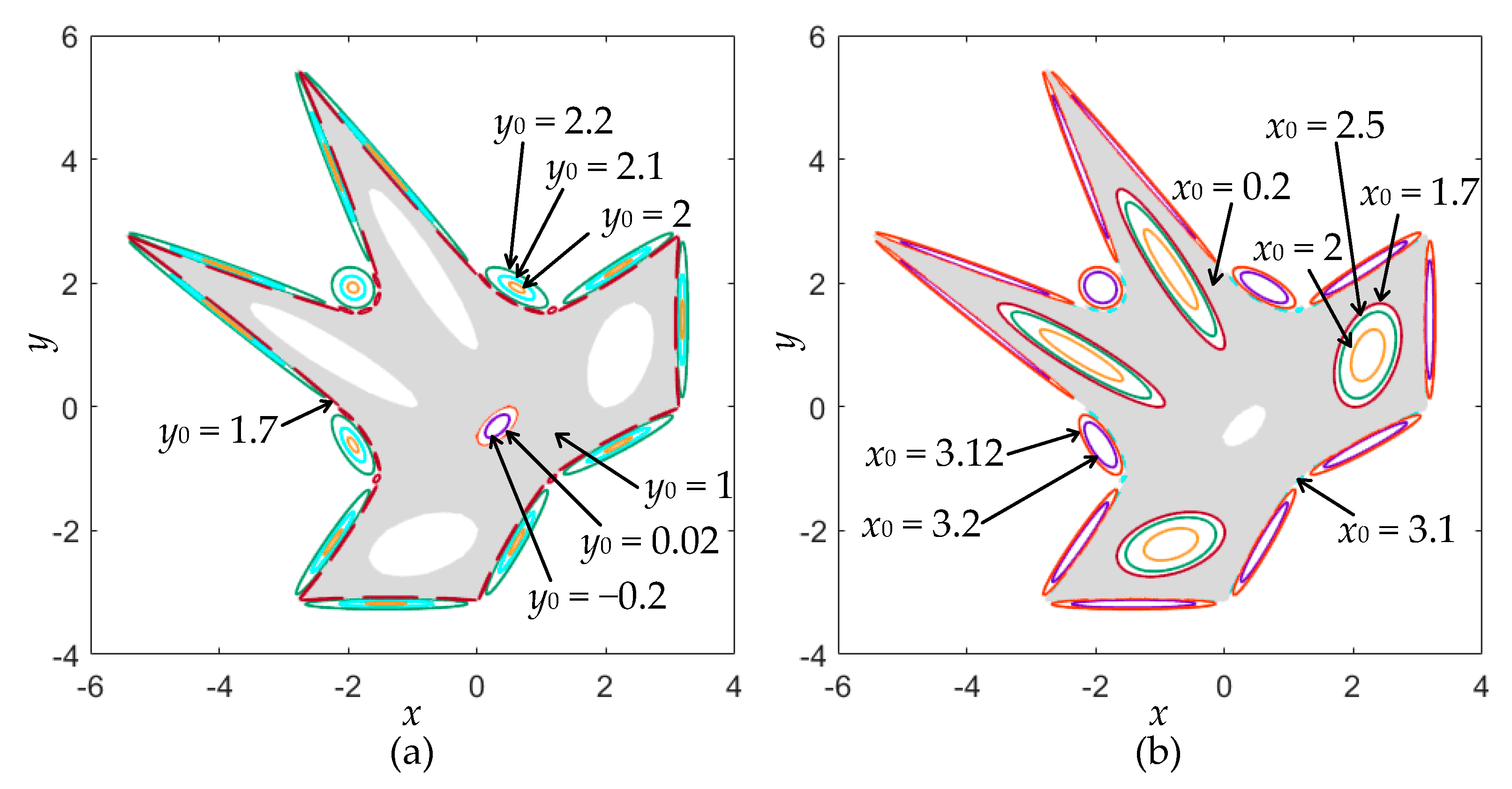
3. Initial Values-Related Coexisting Infinite Orbits

The coexistence of infinite attractors is also called the phenomenon of extreme multistability, which has been reported in numerous memristor-based dynamical circuits and systems [14,15,16]. Mostly this phenomenon occurs in continuous dynamical systems of at least four dimensions. Hence the finding of coexisting infinite orbits in the area-preserving Lozi map is greatly significant.

3.1. Coexisting Chaotic and Quasi-Periodic Orbits

To explore the properties of the area-preserving Lozi map, we inspect its initial values-related dynamical behaviors via the dynamical map, the bifurcation diagram and the phase diagram. The control parameter a is fixed as 1.2. Note that the control parameter of b = −1 is kept unchanged to make sure the Lozi map is area-preserving.
The largest LE (LLE) is a valuable indicator of chaos, and a colorful kinetic map can be plotted in the initial value plane by computing the values of LLE of a discrete map. Figure 5 (middle) displays the kinetic map of the area-preserving Lozi map with the initial value ranges of x0 ∈ [−9, 9] and y0 ∈ [−9, 9]. The initial value ranges emerging from the moving orbits with different values of LLE are labeled by different colors. The magenta–red–yellow, labeled as positive, represents the chaos areas and the dark, labeled as zero, represents the quasi-period and period areas. As can be observed, the kinetic map possesses a complicated fractal structure and smooth boundaries.
In terms of determining an initial value and taking another initial value as a bifurcation parameter, the initial value-related bifurcation diagrams of state x with respect to two initial values x0 and y0 are displayed in Figure 5 (left and bottom). Figure 5 (left) shows the local bifurcation diagram for fixed x0 = 0.5 and variable y0 ∈ [−2.6, 2.2], whereas Figure 5 (bottom) shows the local bifurcation diagram for fixed y0 = 0.5 and variable x0 ∈ [−2.8, 3.2]. The bifurcation diagrams intuitively manifest the dynamical transition from the quasi-periodic route to chaos as the initial values x0 and y0 individually change, resulting in the coexistence of infinite orbits.
The phase diagram can reflect the moving orbits with different topologies, which is suitable to reveal the coexisting behaviors. With the bifurcation diagram given in Figure 5 (left), the phase diagrams under several different initial values y0 are depicted in Figure 6a, from which seven different chaotic and quasi-periodic orbits can be observed. In the same way, with the bifurcation diagram given in Figure 5 (bottom), the phase diagrams under several different initial values x0 are depicted in Figure 6b, from which seven different chaotic and quasi-periodic orbits can also be observed. Note that the chaotic orbit behaves like a chaotic sea, distributed in a determined region, and the quasi-periodic orbit appears as a closed torus. Therefore, the coexistence of a chaotic orbit with a fractal pattern and vast quasi-periodic orbits with different topologies can be disclosed in the area-preserving Lozi map.

3.2. Coexisting Chaotic and Periodic Orbits

To further demonstrate the coexisting infinite orbits, the control parameter is set as a = 1 for the area-preserving Lozi map. Similar to the results in Figure 5, Figure 7 (middle) plots the kinetic map of the area-preserving Lozi map with the initial value ranges of x0 ∈ [−9, 9] and y0 ∈ [−9, 9]. The colorful areas in the initial value planes denote the same moving orbits as those used in Figure 5. As can be seen, the kinetic map in Figure 7 (middle) has a fractal structure different from that of Figure 5.
For this case, when fixing an initial value and taking another initial value as a bifurcation parameter, the initial value-related bifurcation diagrams of state x with respect to two initial values x0 and y0 are displayed in Figure 7 (left and bottom). Figure 7 (left) shows the local bifurcation diagram for fixed x0 = 0.5 and variable y0 ∈ [−7.5, 7], whereas Figure 7 (bottom) shows the local bifurcation diagram for fixed y0 = 0.5 and variable x0 ∈ [−5.4, 6]. Different from the bifurcation diagrams in Figure 5 (left and bottom), the bifurcation diagrams embody the dynamical transition from the periodic route to chaos as the initial values x0 and y0 individually change.
Based on the bifurcation diagrams given in Figure 7, the phase diagrams initiated by different initial values are shown in Figure 8. Figure 8a gives eight kinds of coexisting orbits under a different initial value y0 with x0 = 0.5, and Figure 8b shows seven kinds of coexisting orbits under a different initial value x0 with y0 = 0.5. Therefore, the coexistence of chaotic and periodic orbits with different types and topologies can be disclosed in the area-preserving Lozi map as well. It is stressed that the periodic orbit given in Figure 8 only manifests as some discrete points, whereas the quasi-periodic orbit appears as a closed torus, shown in Figure 6.
Consequently, when the Lozi map is area-preserving, its moving orbits are extremely dependent on its initial values and present period, quasi-period and chaos, with different types and topologies. In other words, the emergence of extreme multistability appears in the area-preserving Lozi map.

3.3. Initial Values-Switched Iterative Sequences

Corresponding to the results in Figure 6 and Figure 8, the initial value-related iterative sequences can be obtained from the area-preserving Lozi map. For fixed a = 1.2, four sets of initial values, (0.5, 0.5), (0.5, 0.6), (0.4, 0.5) and (0.6, 0.5), are selected. Meanwhile, for determined a = 1, another four sets of initial values, (0.5, 0.3), (0.5, 0.4), (0.4, 0.5) and (0.6, 0.5), are chosen. For these sets of initial values, all the iterative sequences are chaotic, and they can be depicted in Figure 9 by numerical simulations.
Except for the chaotic sequences, the area-preserving Lozi map can also produce quasi-periodic and periodic sequences. For fixed a = 1.2, the initial values are set to (0.5, 1.8), (0.5, 1.9), (1.8, 0.5), and (2.2, 0.5), respectively. In these cases, four sets of quasi-periodic sequences are generated and shown in Figure 10a. Thereafter, for fixed a = 1, the initial values are assigned as (0.5, 3.1), (0.5, 3.2), (2.2, 0.5), and (4.6, 0.5), respectively. In these cases, four sets of periodic sequences are generated and shown in Figure 10b.

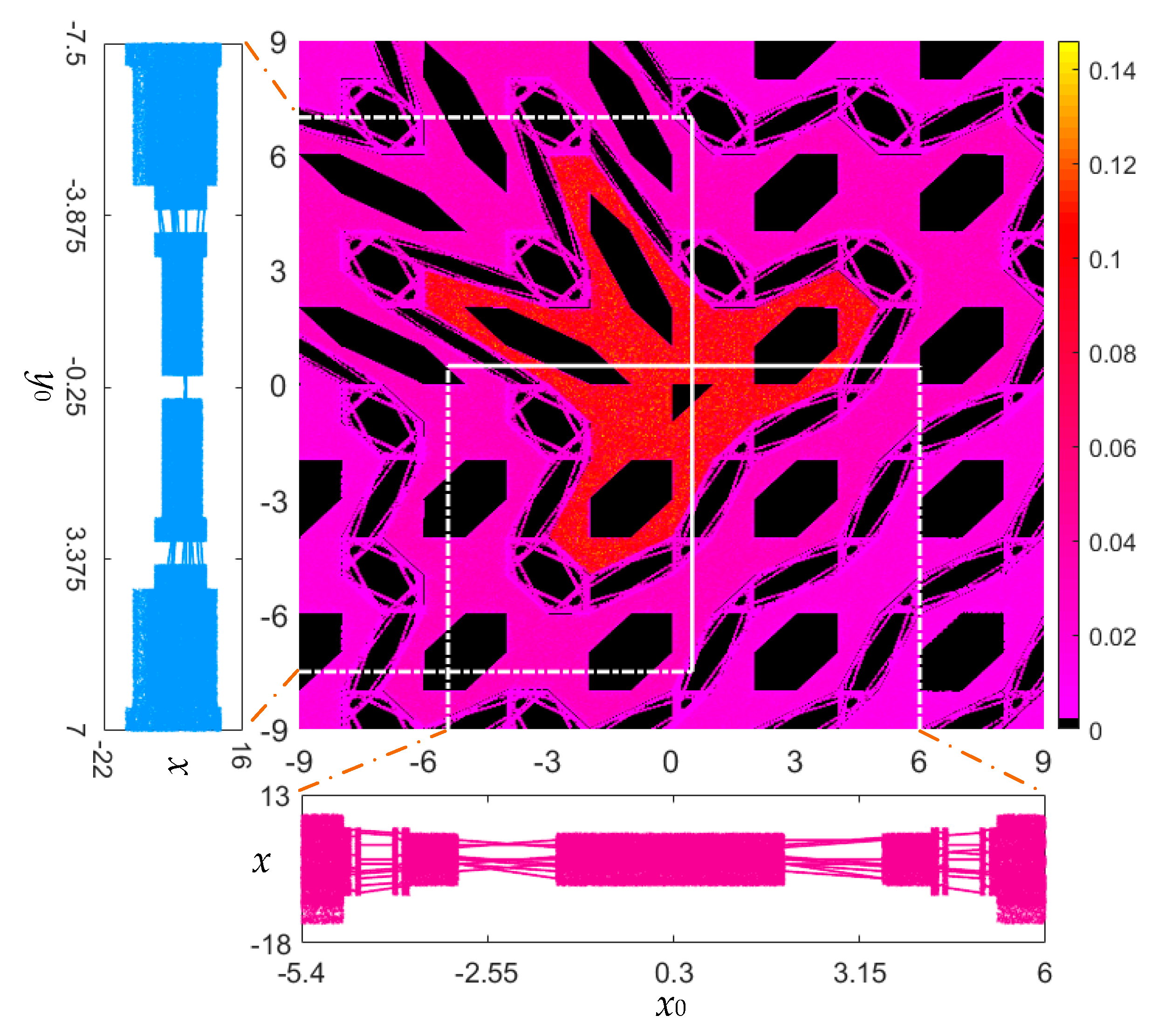
4. Initial Values-Related Complexity

The spectral entropy(SE) and sample entropy (SampEn) are two useful measures of chaos, which can be used to quantitatively calculate the complexity of the coexisting infinite orbits.

4.1. SE-Based Complexity

The SE indicates the disorder of time sequences using an algorithm to measure complexity based on the Fourier transformation [30]. The higher the SE is, the higher the complexity of the time sequences will be.
For a set of time sequences {xn, n = 0, 1, 2, …, N−1} with a length of N, a new discrete number of length N is obtained by subtracting the mean of this dataset from each datum, which is described as
x n = x n n = 0 N 1 x n N
Denote Xk as the discrete Fourier transform of xn. This yields
X k = n = 0 N 1 x n e j 2 π n k / N
in which k = 0, 1, 2, …, N − 1 and j is the unit imaginary. The probability of the power spectrum is defined by
P k = | X k | 2 k = 0 N / 2 1 | X k | 2
Therefore, the normalization spectral entropy can be obtained as
SE = k = 0 N / 2 1 | P k ln ( P k ) | ln ( N / 2 )
where Pk = 0 needs to be removed, or let PklnPk = 0 when Pk = 0. According to the definition of SE, the SE-based complexity can be obtained when the time sequences of state x are selected for the area-preserving Lozi map.
Following the kinetic map in Figure 5, the initial value ranges for the area-preserving Lozi map are also considered as x0 ∈ [−9, 9] and y0 ∈ [−9, 9]. The SE-based complexity distributed in the initial value plane is shown in Figure 11. It is not difficult to find that the SE-based complexity distribution is consistent with the kinetic map in Figure 5 (middle).

4.2. SampEn-Based Complexity

The sample entropy (SampEn) is proposed by reference to the approximate entropy and can reflect the regularity of time sequences [31]. When evaluating sequence complexity, a larger SampEn indicates lower regularity, i.e., greater complexity.
In the same way, consider a set of time sequences {xn, n = 1, 2, 3, …, N} with a length of N. This set of time sequences constructs the (Nm + 1) m-dimensional vectors Xm(i), where Xm(i) = {xi, xi+1, …, xi+m–1}, 1 ≤ iNm + 1. The distance between two vectors Xm(i) and Xm(j) is defined as the absolute value of the maximum difference in the corresponding element, i.e., d[Xm(i), Xm(j)] = max{|x(i + k) − x(j + k)|}, where 0 ≤ km − 1. The Bi is the number of d[Xm(i), Xm(j)] < r (1 ≤ jNm, ij). Define (Nm + 1)−1 times Bi as
B i m ( r ) = 1 N m 1 B i
and define the probability B(m)(r) that two sequences will match for m points as
B ( m ) ( r ) = 1 N m i = 1 N m B i m ( r )
Similarly, Xm+1(i) is (m +1)-dimensional vectors and Ai is the number of d[Xm+1(i), Xm+1(j)] < r. The (Nm + 1)−1 times Ai and the probability, A(m)(r), that two sequences will match for m +1 points are
A i m ( r ) = 1 N m 1 A i
A ( m ) ( r ) = 1 N m i = 1 N m A i m ( r )
Then, when N is finite, the sample entropy can be calculated by
SampEn = ln [ A m ( r ) B m ( r ) ]
where m = 2 and r = 0.2 times the standard deviation in our experiment based on previous studies [32].
The time sequences of state x generated by the area-preserving Lozi map are presumed to be the measurable sequences. According to the kinetic map in Figure 5, the initial value ranges are also considered as x0 ∈ [−9, 9] and y0 ∈ [−9, 9]. The SampEn-based complexity distributed in the initial value plane is plotted in Figure 12. Comparing the results in Figure 11 and Figure 12, the SE-based complexity and SampEn-based complexity have the same distribution in the initial value plane.

5. Hardware Experiment

To physically implement the simple area-preserving Lozi map, a digital microcontroller-based hardware platform is developed. It mainly includes the microcontroller STM32F407VET6 (ARM 32-bit Cortex™-M4 CPU), a D/A converter TLV5618 (12-bit) and a unipolar/bipolar conversion circuit consisting of operational amplifier and resistor. The STM32F4 series chip with flexible pin configuration is easy to weld, which allows us to design a feature-rich printed circuit board (PCB) by matching different peripheral circuits for multiple engineering applications. Of course, in order to achieve more complex chaos-based applications, the raspberry pi board with superior performance can be used to complete the physical implementation by referring to [33].
The model equations, control parameters and initial values are written using C language, and the program is downloaded to the microcontroller. For convenience, Algorithm 1 lists the pseudocode of the microcontroller-based main program [34]. Then, the time-domain waveforms generated by the hardware platform can be clearly observed in the oscilloscope. The screenshot of the four-channel waveforms obtained by the oscilloscope and experimental hardware are shown in Figure 13.
Algorithm 1 The microcontroller-based main program
Initialize the microcontroller and configure the output pins;
Set the length N of sequences, the Number M of interpolation;
Set intermediate variables step1,2,3,4, temp1,2,3,4 and value1,2,3,4;
while true
 Set four sets of (ai, bi, xi,0, yi,0) (i = 1,2,3,4);
for i = 1 to N
   //system equation
   x1,i+1 = 1 − a1|x1,i| + y1,i; y1,i+1 = b1×1,i;
   …
   x4,i+1 = 1 − a4|x4,i| + y4,i; y4,i+1 = b4×4,i;
   //interpolation
   step1 = (x1,i+1x1,i)/M; … step4 = (x4,i+1x4,i)/M;
   for j = 0 to M − 1
    temp1 = x1,i + jstep1; value1 = (temp1 + 15)*4096/30;
    …
    temp4 = x4,i + jstep4; value4 = (temp4 + 15)*4096/30;
    Transfer the value1,2,3,4 to TLV5618;
   end
end
With the digital hardware platform, the discrete iterative sequences for two concerned cases are measured experimentally. Corresponding to the numerical results in Figure 9 and Figure 10, the initial values-related time-domain waveforms generated from the hardware platform are displayed in Figure 14. The experimental results demonstrate that the chaotic, quasi-periodic and periodic waveforms for fixed a = 1 and 1.2 can be captured by the oscilloscope. Because the sequence sampling is random, the initial values-related time-domain waveforms obtained in the experiments are slightly different from the numerically simulated time-domain waveforms. Ignoring these tiny errors, the experimental results are consistent with the numerical results.

6. Conclusions

In order to explore the initial values-related coexisting infinite orbits in a discrete dynamical system, this paper studied the two-dimensional area-preserving Lozi map under specific parameter settings. Within the control parameter of interest, the area-preserving Lozi map has only a fixed point and operates in a critical state. Since the critical fixed point is extremely sensitive to the initial values, the area-preserving Lozi map can easily generate the initial values-related coexisting infinite orbits, i.e., extreme multistability, including periodic, quasi-periodic and chaotic orbits with different types and topologies. The SE- and SampEn-based complexity distributions were employed to evaluate the dynamical performance of the sequences generated from different initial values. By switching the initial values, the iterative sequences were acquired from the developed hardware experiment platform. Of course, the initial values-switched chaotic iterative sequences are worthy of further study in some practical applications.

Author Contributions

Conceptualization, B.B., H.L.; Methodology, H.L.; Software, H.L., K.L.; Validation, H.L., K.L.; Formal analysis, H.L.; Investigation, H.L.; Writing—original draft preparation, H.L.; Writing—review and editing, M.C., B.B.; Visualization, H.L.; Funding acquisition, B.B., M.C. All authors have read and agreed to the published version of the manuscript.

Funding

This work is supported by the National Natural Science Foundations of China under Grant Nos. 51777016 and 61801054, the Natural Science Foundation of Jiangsu Province, China, under Grant No. BK20191451, and the Postgraduate Education Reform Projects of Jiangsu Province China, under Grant No. KYCX20_2548.

Conflicts of Interest

The authors declare that they have no known competing financial interests or personal relationships that could have appeared to influence the work reported in this paper.

References

  1. Hua, Z.; Zhou, Y.; Bao, B. Two-dimensional sine chaotification system with hardware implementation. IEEE Trans. Ind. Inform. 2020, 16, 887–897. [Google Scholar] [CrossRef]
  2. Wang, N.; Li, C.Q.; Bao, H.; Chen, M.; Bao, B.C. Generating multi-scroll Chua’s attractors via simplified piecewise-linear Chua’s diode. IEEE Trans. Circuits Syst. I Reg. Pap. 2019, 66, 4767–4779. [Google Scholar] [CrossRef] [Green Version]
  3. Lan, R.; He, J.W.; Wang, S.H.; Liu, Y.N.; Luo, X.N. A parameter-selection-based chaotic system. IEEE Trans. Circuits Syst. II Exp. Briefs 2019, 66, 492–496. [Google Scholar] [CrossRef]
  4. Moysis, L.; Volos, C.; Jafari, S.; Munoz-Pacheco, J.M.; Kengne, J.; Rajagopal, K.; Stouboulos, I. Modification of the logistic map using fuzzy numbers with application to pseudorandom number generation and image encryption. Entropy 2020, 22, 474. [Google Scholar] [CrossRef] [Green Version]
  5. Lin, C.-Y.; Wu, J.-L. Cryptanalysis and improvement of a chaotic map-based image encryption system using both plaintext related permutation and diffusion. Entropy 2020, 22, 589. [Google Scholar] [CrossRef]
  6. Ding, L.; Ding, Q. The establishment and dynamic properties of a new 4D hyperchaotic system with its application and statistical tests in gray images. Entropy 2020, 22, 310. [Google Scholar] [CrossRef] [Green Version]
  7. Kocamaz, U.E.; Çiçek, S.; Uyaroğlu, Y. Secure communication with chaos and electronic circuit design using passivity-based synchronization. J. Circuits Syst. Comp. 2018, 27, 1850057. [Google Scholar] [CrossRef]
  8. Lai, Q.; Chen, S. Coexisting attractors generated from a new 4D smooth chaotic system. Int. J. Control Autom. Syst. 2016, 14, 1124–1131. [Google Scholar] [CrossRef]
  9. Zhou, W.; Wang, G.Y.; Shen, Y.R.; Yuan, F.; Yu, S.M. Hidden coexisting attractors in a chaotic system without equilibrium point. Int. J. Bifurc. Chaos 2018, 28, 1830033. [Google Scholar] [CrossRef]
  10. Yuan, F.; Wang, G.; Wang, X. Extreme multistability in a memristor-based multi-scroll hyper-chaotic system. Chaos 2016, 26, 073107. [Google Scholar] [CrossRef]
  11. Chen, M.; Li, M.; Yu, Q.; Bao, B.; Xu, Q.; Wang, J. Dynamics of self-excited attractors and hidden attractors in generalized memristor-based Chua’s circuit. Nonlinear Dyn. 2015, 81, 215–226. [Google Scholar] [CrossRef]
  12. Chen, C.J.; Chen, J.Q.; Bao, H.; Chen, M.; Bao, B.C. Coexisting multi-stable patterns in memristor synapse-coupled Hopfield neural network with two neurons. Nonlinear Dyn. 2019, 95, 3385–3399. [Google Scholar] [CrossRef]
  13. Njitacke, Z.T.; Kengne, J. Complex dynamics of a 4D Hopfield neural networks (HNNs) with a nonlinear synaptic weight: Coexistence of multiple attractors and remerging Feigenbaum trees. AEU Int. J. Electron. Commun. 2018, 93, 242–252. [Google Scholar] [CrossRef]
  14. Bao, B.C.; Xu, Q.; Bao, H.; Chen, M. Extreme multistability in a memristive circuit. Electron. Lett. 2016, 52, 1008–1010. [Google Scholar] [CrossRef]
  15. Bao, B.C.; Jiang, T.; Wang, G.Y.; Jin, P.P.; Bao, H.; Chen, M. Two-memristor-based Chua’s hyperchaotic circuit with plane equilibrium and its extreme multistability. Nonlinear Dyn. 2017, 89, 1157–1171. [Google Scholar] [CrossRef]
  16. Chen, M.; Sun, M.; Bao, H.; Hu, Y.; Bao, B. Flux–Charge analysis of two-memristor-based Chua’s circuit: Dimensionality decreasing model for detecting extreme multistability. IEEE Trans. Ind. Electron. 2020, 67, 2197–2206. [Google Scholar] [CrossRef]
  17. Sausedo-Solorio, J.M.; Pisarchik, A.N. Dynamics of unidirectionally coupled bistable Hénon maps. Phys. Lett. A 2011, 375, 3677–3681. [Google Scholar] [CrossRef]
  18. Pisarchik, A.N. Controlling the multistability of nonlinear systems with coexisting attractors. Phys. Rev. E 2001, 64, 046203. [Google Scholar] [CrossRef]
  19. Natiq, H.; Banerjee, S.; Ariffin, M.R.K.; Said, M.R.M. Can hyperchaotic maps with high complexity produce multistability? Chaos 2019, 29, 011103. [Google Scholar] [CrossRef]
  20. Zhusubaliyev, Z.T.; Mosekilde, E. Multistability and hidden attractors in a multilevel DC/DC converter. Math. Comput. Simul. 2015, 109, 32–45. [Google Scholar] [CrossRef]
  21. Bao, B.C.; Li, H.Z.; Zhu, L.; Zhang, X.; Chen, M. Initial-switched boosting bifurcations in 2D hyperchaotic map. Chaos 2020, 30, 033107. [Google Scholar] [CrossRef] [PubMed]
  22. Zhang, L.-P.; Liu, Y.; Wei, Z.-C.; Jiang, H.-B.; Bi, Q.-S. A novel class of two-dimensional chaotic maps with infinitely many coexisting attractors. Chin. Phys. B 2020, 29, 060501. [Google Scholar] [CrossRef]
  23. Bao, H.; Hua, Z.Y.; Wang, N.; Zhu, L.; Chen, M.; Bao, B.C. Initials-boosted coexisting chaos in a 2D Sine map and its hardware implementation. IEEE Trans. Ind. Inform. 2020. [Google Scholar] [CrossRef]
  24. Lozi, R. Un attracteur étrange (?) du type attracteur de Hénon. J. Phys. Colloq. 1978, 39, 9–10. [Google Scholar] [CrossRef]
  25. Botella–Soler, V.; Castelo, J.M.; Oteo, J.A.; Ros, J. Bifurcations in the Lozi map. J. Phys. A Math. Theor. 2011, 44, 305101. [Google Scholar] [CrossRef] [Green Version]
  26. Rybalova, E.; Semenova, N.; Strelkova, G.; Anishchenko, V. Transition from complete synchronization to spatio-temporal chaos in coupled chaotic systems with nonhyperbolic and hyperbolic attractors. Eur. Phys. J. Spec. Top. 2017, 226, 1857–1866. [Google Scholar] [CrossRef]
  27. Hénon, M. A two-dimensional mapping with a strange attractor. Commun. Math. Phys. 1976, 50, 69–77. [Google Scholar] [CrossRef]
  28. Liu, Z.H.; Chen, S.G. Synchronization of a conservative map. Phys. Rev. E 1997, 56, 1585–1589. [Google Scholar]
  29. Wang, N.; Zhang, G.S.; Bao, H. Infinitely many coexisting conservative flows in a 4D conservative system inspired by LC circuit. Nonlinear Dyn. 2020, 99, 3197–3216. [Google Scholar] [CrossRef]
  30. He, S.B.; Sun, K.H.; Wang, H.H. Complexity analysis and DSP implementation of the fractional-order Lorenz hyperchaotic system. Entropy 2015, 17, 8299–8311. [Google Scholar] [CrossRef] [Green Version]
  31. Richman, J.S.; Moorman, J.R. Physiological time-series analysis using approximate entropy and sample entropy. Am. J. Physiol. Heart Circ. Physiol. 2000, 278, H2039–H2049. [Google Scholar] [CrossRef] [Green Version]
  32. Kaffashi, F.; Foglyano, R.; Wilson, C.G.; Loparo, K.A. The effect of time delay on approximate & sample entropy calculations. Phys. D 2008, 237, 3069–3074. [Google Scholar]
  33. Zambrano-Serrano, E.; Muñoz-Pacheco, J.M.; Campos-Cantón, E. Chaos generation in fractional-order switched systems and its digital implementation. AEU Int. J. Electron. Commun. 2017, 79, 43–52. [Google Scholar] [CrossRef]
  34. Li, H.Z.; Hua, Z.Y.; Bao, H.; Zhu, L.; Chen, M.; Bao, B.C. Two-dimensional memristive hyperchaotic maps and application in secure communication. IEEE Trans. Ind. Electron. 2020. [Google Scholar] [CrossRef]
Figure 1. Chaotic attractor of Lozi map under typical parameter settings (a = 1.7 and b = 0.5).
Entropy 22 01119 g001
Figure 2. Stability distributions for the two fixed points in the control parameter plane of a, b. (a) stability distribution for the fixed point F1; (b) stability distribution for the fixed point F2.
Entropy 22 01119 g002
Figure 3. For fixed (x0, y0) = (0.5, 0.5), bifurcation plots of the area-preserving Lozi map with the increase in the control parameter a. (a) Bifurcation diagram; (b) finite-time LEs.
Entropy 22 01119 g003
Figure 4. Phase orbits with different parameter a. (a) Chaos at a = −0.8; (b) quasi-period at a = −0.5; (c) quasi-period at a = 0.1; (d) chaos at a = 1.2.
Entropy 22 01119 g004
Figure 5. For fixed a = 1.2, b = −1, the colorful kinetic map (middle) determined by computing the values of LLE with respect to (x0, y0) ∈ [−9, 9] × [−9, 9]; local bifurcation diagram (left) for fixed x0 = 0.5 and variable y0 ∈ [−2.6, 2.2]; and local bifurcation diagram (bottom) for fixed y0 = 0.5 and variable x0 ∈ [−2.8, 3.2].
Entropy 22 01119 g005
Figure 6. Coexistence of a chaotic orbit and vast quasi-periodic orbits. (a) Seven kinds of moving orbits under different y0 with x0 = 0.5; (b) seven kinds of moving orbits under different x0 with y0 = 0.5.
Entropy 22 01119 g006
Figure 7. For fixed a = 1, b = −1, the colorful kinetic map (middle) determined by computing the values of LLE with respect to (x0, y0) ∈ [−9, 9] × [−9, 9]; local bifurcation diagram (left) for fixed x0 = 0.5 and variable y0 ∈ [−7.5, 7]; and local bifurcation diagram (bottom) for fixed y0 = 0.5 and variable x0 ∈ [−5.4, 6].
Entropy 22 01119 g007
Figure 8. Coexistence of chaotic and periodic orbits. (a) Eight kinds of coexisting orbits under different y0 with x0 = 0.5; (b) seven kinds of coexisting orbits under different x0 with y0 = 0.5.
Entropy 22 01119 g008
Figure 9. Initial values-related chaotic iterative sequences. (a) Chaotic sequences for a = 1.2; (b) chaotic sequences for a = 1.
Entropy 22 01119 g009
Figure 10. Initial values-related quasi-periodic and periodic iterative sequences. (a) Quasi-periodic sequences for a = 1.2; (b) periodic sequences for a = 1.
Entropy 22 01119 g010
Figure 11. For fixed a = 1.2, b = −1, the colorful SE-based complexity distribution with respect to (x0, y0) ∈ [−9, 9] × [−9, 9].
Entropy 22 01119 g011
Figure 12. For fixed a = 1.2, b = −1, the colorful SampEn-based complexity distribution with respect to (x0, y0) ∈ [−9, 9] × [−9, 9].
Entropy 22 01119 g012
Figure 13. Digital microcontroller-based experiment platform and the displayed four-channel waveforms.
Entropy 22 01119 g013
Figure 14. Initial values-related time-domain waveforms generated from the hardware platform. (a) Chaotic waveforms with a = 1.2; (b) chaotic waveforms for a = 1; (c) quasi-periodic waveforms for a = 1.2; (d) periodic waveforms for a = 1.
Entropy 22 01119 g014

