Numerical Modelling of Microchannel Gas Flows in the Transition Flow Regime Using the Cascaded Lattice Boltzmann Method

Abstract

In this article, a lattice Boltzmann (LB) method for studying microchannel gas flows is developed in the framework of the cascaded collision operator. In the cascaded lattice Boltzmann (CLB) method, the Bosanquet-type effective viscosity is employed to capture the rarefaction effects, and the combined bounce-back/specular-reflection scheme together with the modified second-order slip boundary condition is adopted so as to match the Bosanquet-type effective viscosity. Numerical simulations of microchannel gas flow with periodic and pressure boundary conditions in the transition flow regime are carried out to validate the CLB method. The predicted results agree well with the analytical, numerical, and experimental data reported in the literature.

1. Introduction

Over the last few decades, microscale rarefied gas flows attract considerable research attention owing to the rapid progress of fabrication techniques in micro-electro-mechanical systems (MEMS) (e.g., microchannels, micropipes, microturbines, and microbearings) [1,2,3,4]. Typically, gas flows in microfluidic devices can be characterized by the Knudsen number $Kn=\lambda /H$ (the ratio of the mean free path $\lambda$ of the gas molecules to the characteristic length $H$ of the flow system), which serves as a criterion in indicating the degree of the rarefaction effects of gas flows. Usually, gas flows can be empirically classified as follows [5,6]: Continuum flow ($Kn<0.001$), slip flow ($0.001<Kn<0.1$), transition flow ($0.1<Kn<10$), and free molecular flow ($Kn>10$). It is well accepted that continuum-based Navier–Stokes (NS) equations in conjunction with slip boundary conditions remain valid up to $Kn=0.1$ or thereabouts [6,7]. However, for $Kn>0.1$, the flow characteristics are dominated by the rarefaction effects and the traditional NS equations are no longer valid because the continuum and thermodynamic equilibrium hypotheses break down [3,4], and therefore, the Boltzmann equation (BE) must be considered to analyze such flows [8,9].

For gas flows in MEMS devices where the geometric size of the flow domain is very small, $Kn$ is relatively large, and such flows usually fall into the slip and transition flow regimes [10]. Due to technical advances, gas flows in microfluidic systems have been experimentally studied by many researchers [11,12,13,14]. In addition to the experimental investigations, theoretical and numerical approaches play important roles in studying gas flows in microfluidic systems. As reported by Cercignani [8], the BE is applicable for all flow regimes. Theoretically, in slip and transition flow regimes, gas flows can be described via directly solving the BE or model using the direct simulation Monte Carlo (DSMC) method [15]. However, it has been demonstrated that it is impractical to obtain the BEs solution except for a few cases, and the DSMC method usually suffers from statistical noise and high computational cost in solving practical problems. Therefore, many numerically accurate and efficient methods based on the BE of the kinetic theory have been developed for studying rarefied gas flows [16,17,18,19,20,21]. Among these BE-based numerical methods, the mesoscopic LB method has attracted significant attention in studying microscale rarefied gas flows since 2002 [18,19,22,23,24,25,26,27,28,29,30,31,32,33].

The LB method [34,35,36,37,38,39,40], as a mesoscopic numerical method that originated from lattice gas automata method [41], has been developed into a powerful numerical tool for computational fluid dynamics and beyond. In recent years, the cascaded or central-moments-based lattice Boltzmann (CLB) method [42,43,44,45,46] has also attracted much attention. The CLB method was proposed by Geier et al. [42] in 2006. In this method, the collision process is performed in terms of central moments (moments shifted by the local macroscopic fluid velocity) in an ascending order in a moving reference frame, beginning with the lowest and ending with the highest. The CLB method possesses advantages over the LB method with the Bhatnagar-Gross-Krook (BGK) and traditional multiple-relaxation-time (MRT) collision operators in terms of Galilean invariance and numerical stability [47]. The CLB method represents an alternative approach to enhance the stabilities of the BGK and standard MRT method [48]. In the CLB method, Galilean invariance can be naturally prescribed and different central moments are relaxed in the central-moment space with different rates, which means that the degrees of freedom in the CLB method are enough to adjust higher-order discretization errors that resulted from the implementation of boundary conditions. To the best of our knowledge, there have been no studies on microscale gas flows using the CLB method. Hence, the purpose of this paper is to propose a CLB method for simulating microchannel gas flows in transition flow regime. It is expected that microscale rarefied gas flows in the transition flow regime can be well simulated by the proposed CLB method.

2. The CLB Method

2.1. The CLB Model

In this subsection, the CLB model with a forcing term [43] is introduced. For 2D microscale rarefied gas flows, the two-dimensional nine-velocity (D2Q9) lattice model is adopted. The discrete velocities $\left\{{\mathbf{e}}_i|i=0,1,\dots ,8\right\}$ of the D2Q9 lattice are given by [49]

$${\mathbf{e}}_i=\{\begin{array}{ll}\left(0,0\right),\hfill & i=0,\hfill \\ \left(\cos \left[\left(i-1\right)\pi /2\right],\sin \left[\left(i-1\right)\pi /2\right]\right)c,\hfill & i=1-4,\hfill \\ \left(\cos \left[\left(2i-9\right)\pi /4\right],\sin \left[\left(2i-9\right)\pi /4\right]\right)\sqrt{2}c,\hfill & i=5-8,\hfill \end{array}$$

(1)

where $c={\delta }_x/{\delta }_t$ is the lattice speed, ${\delta }_t$ is the time step, and ${\delta }_x$ is the lattice spacing.

The CLB equation with a forcing term is given by

$$f_i\left(\mathbf{x}+{\mathbf{e}}_i{\delta }_t,t+{\delta }_t\right)=f_i\left(\mathbf{x},t\right)+{\Omega }_i^C|{}_{\left(\mathbf{x},t\right)}+\frac{{\delta }_t}{2}\left[S_i|{}_{\left(\mathbf{x},t\right)}+S_i|{}_{\left(\mathbf{x}+{\mathbf{e}}_i{\delta }_t,t+{\delta }_t\right)}\right]$$

(2)

where $f_i$ is the discrete density distribution function, ${\Omega }_i^C$ is the collision term, and $S_i$ is the forcing term. In the cascaded collision model, the collision term ${\Omega }_i^C$ can be expressed as ${\Omega }_i^C\equiv {\Omega }_i^C\left(f,\widehat{\mathbf{g}}\right)={\left(\mathbf{K}\cdot \widehat{\mathbf{g}}\right)}_i$, in which $f=|f\rangle ={\left(f_0,f_1,\dots ,f_8\right)}^{\mathrm{T}}$, and $\widehat{\mathbf{g}}=|\widehat{g}\rangle ={\left({\widehat{g}}_0,{\widehat{g}}_1,\dots ,{\widehat{g}}_8\right)}^{\mathrm{T}}$ ($\left\{{\widehat{g}}_i\right\}$ are unknown collision kernels. $\mathbf{K}$ is an orthogonal matrix given by ($c=1$) [43]

$$\begin{array}{l}\mathbf{K}=[|1\rangle ,|e_x\rangle ,|e_y\rangle ,3|e_x^2+e_y^2\rangle -4|1\rangle ,|e_x^2-e_y^2\rangle ,|e_x{e}_y\rangle ,-3|e_x^2{e}_y\rangle +2|e_y\rangle ,\\ -3|e_x{e}_y^2\rangle +2|e_x\rangle ,9|e_x^2{e}_y^2\rangle -6|e_x^2+e_y^2\rangle +4|1\rangle ]\end{array}$$

$$=\left[\begin{array}{rrrrrrrrr}\hfill 1& \hfill 0& \hfill 0& \hfill -4& \hfill 0& \hfill 0& \hfill 0& \hfill 0& \hfill 4\\ \hfill 1& \hfill 1& \hfill 0& \hfill -1& \hfill 1& \hfill 0& \hfill 0& \hfill 2& \hfill -2\\ \hfill 1& \hfill 0& \hfill 1& \hfill -1& \hfill -1& \hfill 0& \hfill 2& \hfill 0& \hfill -2\\ \hfill 1& \hfill -1& \hfill 0& \hfill -1& \hfill 1& \hfill 0& \hfill 0& \hfill -2& \hfill -2\\ \hfill 1& \hfill 0& \hfill -1& \hfill -1& \hfill -1& \hfill 0& \hfill -2& \hfill 0& \hfill -2\\ \hfill 1& \hfill 1& \hfill 1& \hfill 2& \hfill 0& \hfill 1& \hfill -1& \hfill -1& \hfill 1\\ \hfill 1& \hfill -1& \hfill 1& \hfill 2& \hfill 0& \hfill -1& \hfill -1& \hfill 1& \hfill 1\\ \hfill 1& \hfill -1& \hfill -1& \hfill 2& \hfill 0& \hfill 1& \hfill 1& \hfill 1& \hfill 1\\ \hfill 1& \hfill 1& \hfill -1& \hfill 2& \hfill 0& \hfill -1& \hfill 1& \hfill -1& \hfill 1\end{array}\right]$$

(3)

By introducing a transformed distribution function ${\overline{f}}_i=f_i-0.5{\delta }_t{S}_i$, the implicitness of the CLB Equation (2) can be eliminated, which yields

$${\tilde{\overline{f}}}_i\left(\mathbf{x},t\right)={\overline{f}}_i\left(\mathbf{x},t\right)+{\Omega }_i^C|{}_{\left(\mathbf{x},t\right)}+{\delta }_t{S}_i|{}_{\left(\mathbf{x},t\right)},$$

(4)

$${\overline{f}}_i\left(\mathbf{x}+{\mathbf{e}}_i{\delta }_t,t+{\delta }_t\right)={\tilde{\overline{f}}}_i\left(\mathbf{x},t\right),$$

(5)

where Equations (4) and (5) denote the collision and streaming steps, respectively, and ${\tilde{\overline{f}}}_i$ is the post-collision distribution function. According to the orthogonal matrix $\mathbf{K}$, the collision step (4) can be expanded as follows [43]:

$${\tilde{\overline{f}}}_0={\overline{f}}_0+\left[{\widehat{g}}_0-4\left({\widehat{g}}_3-{\widehat{g}}_8\right)\right]+{\delta }_t{S}_0,$$

$${\tilde{\overline{f}}}_1={\overline{f}}_1+\left[{\widehat{g}}_0+{\widehat{g}}_1-{\widehat{g}}_3+{\widehat{g}}_4+2\left({\widehat{g}}_7-{\widehat{g}}_8\right)\right]+{\delta }_t{S}_1,$$

$${\tilde{\overline{f}}}_2={\overline{f}}_2+\left[{\widehat{g}}_0+{\widehat{g}}_2-{\widehat{g}}_3-{\widehat{g}}_4+2\left({\widehat{g}}_6-{\widehat{g}}_8\right)\right]+{\delta }_t{S}_2,$$

$${\tilde{\overline{f}}}_3={\overline{f}}_3+\left[{\widehat{g}}_0-{\widehat{g}}_1-{\widehat{g}}_3+{\widehat{g}}_4-2\left({\widehat{g}}_7+{\widehat{g}}_8\right)\right]+{\delta }_t{S}_3,$$

$${\tilde{\overline{f}}}_4={\overline{f}}_4+\left[{\widehat{g}}_0-{\widehat{g}}_2-{\widehat{g}}_3-{\widehat{g}}_4-2\left({\widehat{g}}_6+{\widehat{g}}_8\right)\right]+{\delta }_t{S}_4,$$

(6)

$${\tilde{\overline{f}}}_5={\overline{f}}_5+\left[{\widehat{g}}_0+{\widehat{g}}_1+{\widehat{g}}_2+2{\widehat{g}}_3+{\widehat{g}}_5-{\widehat{g}}_6-{\widehat{g}}_7+{\widehat{g}}_8\right]+{\delta }_t{S}_5,$$

$${\tilde{\overline{f}}}_6={\overline{f}}_6+\left[{\widehat{g}}_0-{\widehat{g}}_1+{\widehat{g}}_2+2{\widehat{g}}_3-{\widehat{g}}_5-{\widehat{g}}_6+{\widehat{g}}_7+{\widehat{g}}_8\right]+{\delta }_t{S}_6,$$

$${\tilde{\overline{f}}}_7={\overline{f}}_7+\left[{\widehat{g}}_0-{\widehat{g}}_1-{\widehat{g}}_2+2{\widehat{g}}_3+{\widehat{g}}_5+{\widehat{g}}_6+{\widehat{g}}_7+{\widehat{g}}_8\right]+{\delta }_t{S}_7,$$

$${\tilde{\overline{f}}}_8={\overline{f}}_8+\left[{\widehat{g}}_0+{\widehat{g}}_1-{\widehat{g}}_2+2{\widehat{g}}_3-{\widehat{g}}_5+{\widehat{g}}_6-{\widehat{g}}_7+{\widehat{g}}_8\right]+{\delta }_t{S}_8.$$

The collision kernels $\left\{{\widehat{g}}_i|i=0,1,\dots ,8\right\}$ are [43]:

$${\widehat{g}}_0={\widehat{g}}_1={\widehat{g}}_2=0,$$

$${\widehat{g}}_3=\frac{s_3}{12}\left\{\frac{2}{3}\rho +\rho \left(u_x^2+u_y^2\right)-\left({{\widehat{\overline{\kappa }}}^{\prime }}_{xx}+{{\widehat{\overline{\kappa }}}^{\prime }}_{yy}\right)-\frac{1}{2}\rho \left(2F_x{u}_x+2F_y{u}_y\right)\right\},$$

$${\widehat{g}}_4=\frac{s_4}{4}\left\{\rho \left(u_x^2-u_y^2\right)-\left({{\widehat{\overline{\kappa }}}^{\prime }}_{xx}-{{\widehat{\overline{\kappa }}}^{\prime }}_{yy}\right)-\frac{1}{2}\rho \left(2F_x{u}_x-2F_y{u}_y\right)\right\},$$

$${\widehat{g}}_5=\frac{s_5}{4}\left\{\rho u_x{u}_y-{{\widehat{\overline{\kappa }}}^{\prime }}_{xy}-\frac{1}{2}\rho \left(F_x{u}_y+F_y{u}_x\right)\right\},$$

$$\begin{array}{c}{\widehat{g}}_6=\frac{s_6}{4}\left\{2\rho u_x^2{u}_y+{{\widehat{\overline{\kappa }}}^{\prime }}_{xxy}-2u_x{{\widehat{\overline{\kappa }}}^{\prime }}_{xy}-u_y{{\widehat{\overline{\kappa }}}^{\prime }}_{xx}-\frac{1}{2}\rho \left(F_y{u}_x^2+2F_x{u}_x{u}_y\right)\right\}\\ -\frac{1}{2}{u}_y\left(3{\widehat{g}}_3+{\widehat{g}}_4\right)-2u_x{\widehat{g}}_5,\end{array}$$

(7)

$$\begin{array}{c}{\widehat{g}}_7=\frac{s_7}{4}\left\{2\rho u_x{u}_y^2+{{\widehat{\overline{\kappa }}}^{\prime }}_{xyy}-2u_y{{\widehat{\overline{\kappa }}}^{\prime }}_{xy}-u_x{{\widehat{\overline{\kappa }}}^{\prime }}_{yy}-\frac{1}{2}\rho \left(F_x{u}_y^2+2F_y{u}_y{u}_x\right)\right\}\\ -\frac{1}{2}{u}_x\left(3{\widehat{g}}_3-{\widehat{g}}_4\right)-2u_y{\widehat{g}}_5,\end{array}$$

$$\begin{array}{c}{\widehat{g}}_8=\frac{s_8}{4}\{\frac{1}{9}\rho +3\rho u_x^2{u}_y^2-\left[{{\widehat{\overline{\kappa }}}^{\prime }}_{xxyy}-2u_x{{\widehat{\overline{\kappa }}}^{\prime }}_{xyy}-2u_y{{\widehat{\overline{\kappa }}}^{\prime }}_{xxy}+u_x^2{{\widehat{\overline{\kappa }}}^{\prime }}_{yy}+u_y^2{{\widehat{\overline{\kappa }}}^{\prime }}_{xx}+4u_x{u}_y{{\widehat{\overline{\kappa }}}^{\prime }}_{xy}\right]\\ -\frac{1}{2}\rho (2F_x{u}_x{u}_y^2+2F_y{u}_y{u}_x^2)\}-2{\widehat{g}}_3-\frac{1}{2}{u}_y^2(3{\widehat{g}}_3+{\widehat{g}}_4)-\frac{1}{2}{u}_x^2(3{\widehat{g}}_3+{\widehat{g}}_4)\\ -4u_x{u}_y{\widehat{g}}_5-2u_y^{}{\widehat{g}}_6-2u_x^{}{\widehat{g}}_7,\end{array}$$

where $\mathbf{F}=\left(F_x,F_y\right)$ is the external force, $\left\{s_i|i=3,4,\dots ,8\right\}$ are relaxation rates, and ${{\widehat{\overline{\kappa }}}^{\prime }}_{x^m{y}^n}=\langle e_x^m{e}_y^n|\overline{f}\rangle$ ($m,n\in \left\{0,1,2\right\}$, and $\langle e_x^m{e}_y^n|\overline{f}\rangle$ denotes the inner product ${\displaystyle {\sum }_{i=0}^8{e}_{ix}^m{e}_{iy}^n{\overline{f}}_i}$) is the raw moment of the transformed distribution functions of order $(m+n)$. The discrete central moment of the transformed distribution functions of order $(m+n)$ is defined by ${\widehat{\overline{\kappa }}}_{x^m{y}^n}=\langle {\left(e_x-u_x\right)}^m{\left(e_y-u_y\right)}^n|\overline{f}\rangle$ [42,43]. In computations, the collision step of the CLB equation is actually performed in terms of the raw moments. The collision kernel ${\widehat{g}}_i$ satisfies ${\widehat{g}}_i\equiv {\widehat{g}}_i\left(\mathbf{f},{\widehat{g}}_{\beta }\right)$, $\beta =0,1,\dots ,i-1$. For the D2Q9 model, the raw moments ${{\widehat{\overline{\kappa }}}^{\prime }}_{x^m{y}^n}$ can be expressed as follows:

$${{\widehat{\overline{\kappa }}}^{\prime }}_0=\langle 1|\overline{f}\rangle =\rho ,$$

$${{\widehat{\overline{\kappa }}}^{\prime }}_x=\langle e_x|\overline{f}\rangle =\rho u_x-\frac{1}{2}\rho F_x,$$

$${{\widehat{\overline{\kappa }}}^{\prime }}_y=\langle e_y|\overline{f}\rangle =\rho u_y-\frac{1}{2}\rho F_y,$$

$${{\widehat{\overline{\kappa }}}^{\prime }}_{xx}=\langle e_x^2|\overline{f}\rangle ={\displaystyle \sum _i^{\left\{1,3,5,6,7,8\right\}}{\overline{f}}_i},$$

$${{\widehat{\overline{\kappa }}}^{\prime }}_{yy}=\langle e_y^2|\overline{f}\rangle ={\displaystyle \sum _i^{\left\{2,4,5,6,7,8\right\}}{\overline{f}}_i},$$

(8)

$${{\widehat{\overline{\kappa }}}^{\prime }}_{xy}=\langle e_x{e}_y^{}|\overline{f}\rangle ={\displaystyle \sum _i^{\left\{5,7\right\}}{\overline{f}}_i}-{\displaystyle \sum _i^{\left\{6,8\right\}}{\overline{f}}_i},$$

$${{\widehat{\overline{\kappa }}}^{\prime }}_{xxy}=\langle e_x^2{e}_y^{}|\overline{f}\rangle ={\displaystyle \sum _i^{\left\{5,6\right\}}{\overline{f}}_i}-{\displaystyle \sum _i^{\left\{7,8\right\}}{\overline{f}}_i},$$

$${{\widehat{\overline{\kappa }}}^{\prime }}_{xyy}=\langle e_x^{}{e}_y^2|\overline{f}\rangle ={\displaystyle \sum _i^{\left\{5,8\right\}}{\overline{f}}_i}-{\displaystyle \sum _i^{\left\{6,7\right\}}{\overline{f}}_i},$$

$${{\widehat{\overline{\kappa }}}^{\prime }}_{xxyy}=\langle e_x^2{e}_y^2|\overline{f}\rangle ={\displaystyle \sum _i^{\left\{5,6,7,8\right\}}{\overline{f}}_i},$$

The forcing term $\mathbf{S}=|S\rangle$ can be obtained via $\mathbf{S}={\mathbf{T}}^{-1}\widehat{\mathbf{S}}$, where $\widehat{\mathbf{S}}=|{\widehat{S}}_i\rangle$ is given by

$$\widehat{\mathbf{S}}=\left[\begin{array}{c}0\\ \rho F_x\\ \rho F_y\\ 2\rho \left(u_x{F}_x+u_y{F}_y\right)\\ 2\rho \left(u_x{F}_x-u_y{F}_y\right)\\ \rho \left(u_x{F}_y+u_y{F}_x\right)\\ \rho F_y{u}_x^2+2\rho F_x{u}_x{u}_y\\ \rho F_x{u}_y^2+2\rho F_y{u}_y{u}_x\\ 2\rho F_x{u}_x{u}_y^2+2\rho F_y{u}_y{u}_x^2\end{array}\right].$$

(9)

The transformation matrix $\mathbf{T}$ is

$$\mathbf{T}=[|1\rangle ,|e_x\rangle ,|e_y\rangle ,|e_x^2+e_y^2\rangle ,|e_x^2-e_y^2\rangle ,|e_x{e}_y\rangle ,|e_x^2{e}_y\rangle ,{|e_x{e}_y^2\rangle ,|e_x^2{e}_y^2\rangle ]}^{\mathrm{T}}.$$

(10)

The equilibrium distribution function $f_i^{eq}$ can be obtained via ${\mathbf{f}}^{eq}={\mathbf{T}}^{-1}{\widehat{\mathbf{f}}}^{eq}$, in which ${\widehat{\mathbf{f}}}^{eq}=|{\widehat{f}}_i^{eq}\rangle$ is given by

$${\widehat{\mathbf{f}}}^{eq}=\left[\begin{array}{c}\rho \\ \rho u_x\\ \rho u_y\\ \frac{2}{3}\rho +\rho \left(u_x^2+u_y^2\right)\\ \rho \left(u_x^2-u_y^2\right)\\ \rho u_x^{}{u}_y\\ \frac{1}{3}\rho u_y+\rho u_x^2{u}_y\\ \frac{1}{3}\rho u_x+\rho u_x{u}_y^2\\ \frac{1}{9}\rho +\frac{1}{3}\rho \left(u_x^2+u_y^2\right)+\rho u_x^2{u}_y^2\end{array}\right].$$

(11)

The fluid density $\rho$ and velocity $u$ are given by

$$\rho ={\displaystyle \sum _{i=0}^8{f}_i}={\displaystyle \sum _{i=0}^8{\overline{f}}_i},$$

(12)

$$\rho u={\displaystyle \sum _{i=0}^8{e}_i{f}_i}={\displaystyle \sum _{i=0}^8{e}_i{\overline{f}}_i}+\frac{{\delta }_t}{2}\rho F.$$

(13)

The pressure $p$ is defined by $p=\rho c_s^2$, where $c_s^{}=c/\sqrt{3}$ is the lattice sound speed. The dynamic viscosity $\mu$ and bulk viscosity $\mathsf{\xi }$ are given by

$$\mu =\rho c_s^2\left(\frac{1}{s_{\upsilon }}-\frac{1}{2}\right){\delta }_t,\mathsf{\xi }=c_s^2\left(\frac{1}{s_b}-\frac{1}{2}\right){\delta }_t,$$

(14)

respectively. In the CLB model, $s_4=s_5=s_{\upsilon }$ and $s_3=s_b$. The cascaded collision term ${\Omega }_i^C$ is constructed in a way that the central moments are relaxed independently at different relaxation rates. From this point of view, the CLB method can be regarded as an MRT scheme based on central moments.

2.2. Bosanquet-Type Effective Viscosity

For microscale gas flows, $Kn$ is the most important characteristic parameter. In order to extend the CLB model to simulate microscale gas flows in the slip and transition flow regimes, the relationship between $\mu$ and $Kn$ should be given appropriately. In the kinetic theory, the relationship between $\mu$ and the mean free path $\lambda$ can be expressed as [8]

$$\lambda =\frac{\mu }{p}\sqrt{\frac{\pi RT}{2}}.$$

(15)

As reported in [25], the above relationship is only valid for rarefied gas flows in unbounded systems. In bounded systems, the relationship given by Equation (15) are questionable because the existence of walls can reduce the local mean free path at the near wall regions [27,29,31]. In order to reflect the influence of the gas molecule/wall interactions, the Bosanquet-type effective viscosity is employed [31,50,51]

$${\mu }_e=\frac{\mu }{1+aKn},$$

(16)

where $a$ is the rarefaction factor. Accordingly, the effective mean free path ${\lambda }_e$ is determined by ${\lambda }_e=\left({\mu }_e/p\right)\sqrt{\pi RT/2}$. The rarefaction factor $a$ depends on $Kn$, but as reported in [51], such a dependence is very weak in the majority of the transition flow regime, suggesting an effective value close to 2. Based on this, we use ${\mu }_e=\mu /\left(1+aKn\right)$ with $\alpha =2$ in the present study. For the D2Q9 model, according to Equations (15) and (16), ${\mu }_e$ can be determined by

$${\mu }_e=\frac{c}{3}\sqrt{\frac{6}{\pi }}\frac{\rho KnH}{1+aKn},$$

(17)

where $H$ is the characteristic length. To produce the Bosanquet-type effective viscosity ${\mu }_e$ in the CLB method, according to Equations (14) and (17), the relaxation rate $s_{\upsilon }$ is given as

$$s_{\upsilon }^{-1}=\frac{1}{2}+\sqrt{\frac{6}{\pi }}\frac{NKn}{\left(1+aKn\right)}.$$

(18)

2.3. Boundary Condition

When the Bosanquet-type effective viscosity is adopted, the following modified second-order slip boundary condition [31] should be considered:

$$u_s=B_1{\sigma }_v{\lambda }_e{\frac{\partial u}{\partial \mathbf{n}}|}_w-B_2{\lambda }_e^2{\frac{{\partial }^{2}u}{\partial {\mathbf{n}}^2}|}_w,$$

(19)

where $u_s$ is the slip velocity, $B_1$ is the first-order slip coefficient, $B_2$ is the second-order slip coefficient, $\mathbf{n}$ is the unit vector normal to the wall, the subscript $w$ represents the quantity at the wall, and ${\sigma }_v=\left(2-\sigma \right)/\sigma$, in which $\sigma$ is the TMAC (tangential momentum accommodation coefficient). To realize the modified second-order slip boundary condition (Equation (19)), the combined bounce-back/specular-reflection (CBBSR) boundary scheme [22,27,31] is adopted. For instance, for slip boundary condition at the bottom wall (placed at $J=0.5$), the unknown distribution functions (${\overline{f}}_2$, ${\overline{f}}_5$, and ${\overline{f}}_6$) at $J=1$ are determined by

$${\overline{f}}_2={\tilde{\overline{f}}}_4,{\overline{f}}_5=r_b{\tilde{\overline{f}}}_7+\left(1-r_b\right){\tilde{\overline{f}}}_8,{\overline{f}}_6=r_b{\tilde{\overline{f}}}_8+\left(1-r_b\right){\tilde{\overline{f}}}_7,$$

(20)

where ${\tilde{\overline{f}}}_i$ ($i=2,5,6$) are the post-collision distribution functions at $J=1$, and $r_b\in \left[0,1\right]$ is the portion of the bounce-back part in the combination. According to [31], the parameter $r_b$ and the relaxation rate $s_q$ ($s_6=s_7=s_q$) should be chosen as follows:

$$r_b=\frac{1}{1+B_1{\sigma }_v\sqrt{\pi /6}},s_q^{-1}=\frac{1}{2}+\frac{3+4\pi {\tilde{\tau }}_q^2{B}_2}{16{\tilde{\tau }}_q},$$

(21)

where ${\tilde{\tau }}_q=s_{\upsilon }^{-1}-0.5$, in which $s_{\upsilon }^{}$ is determined by Equation (18).

3. Numerical Simulations

In this section, the microchannel gas flow with periodic and pressure boundary conditions are studied by the proposed CLB method. In the following simulations, we set ${\delta }_x={\delta }_y={\delta }_t=1$, $B_1=\left(1-0.1817\sigma \right)$, and $B_2=0.55$. The free relaxation rates are selected as $s_3=1.1$ and $s_8=1.2$.

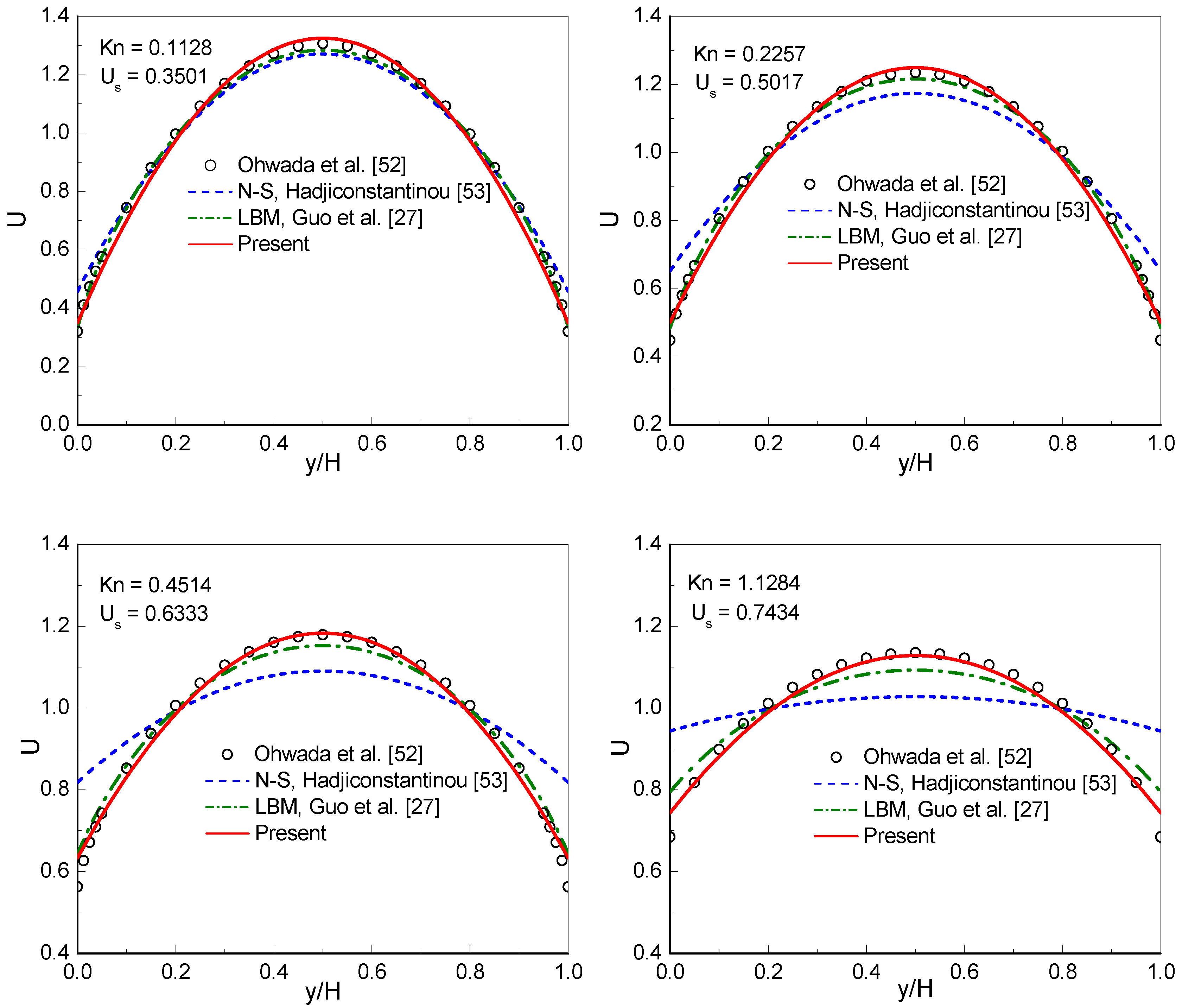
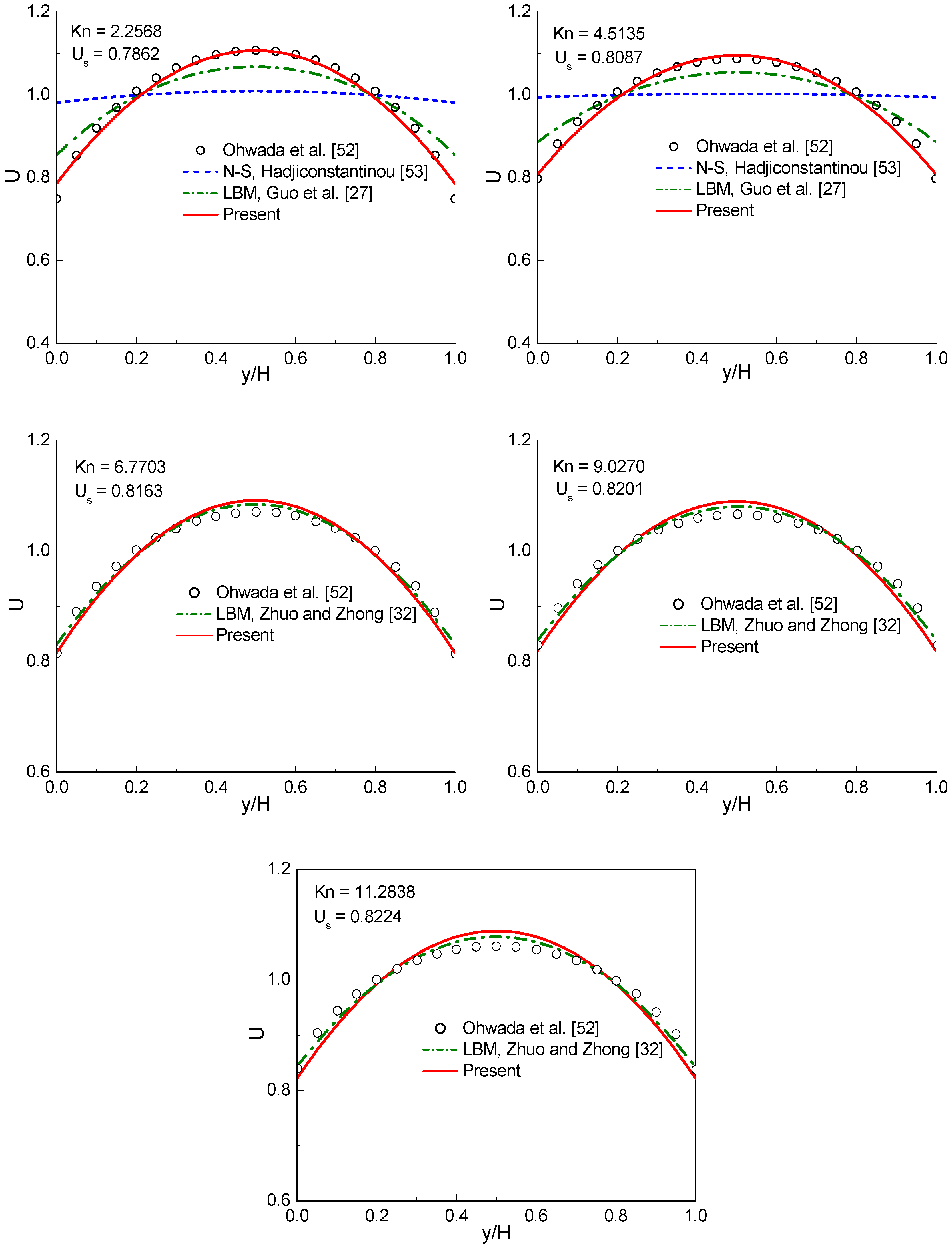
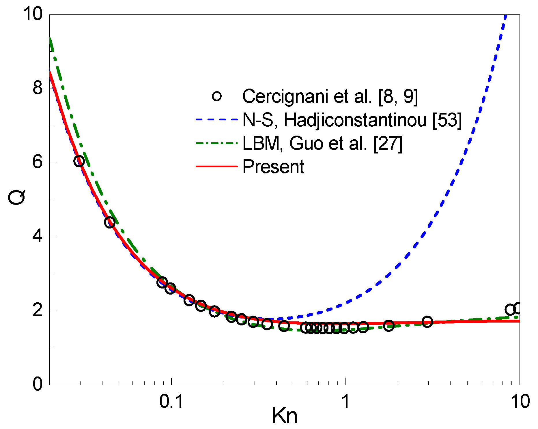
3.1. Microchannel Gas Flow with Periodic Boundary Condition

In this subsection, the microchannel gas flow with periodic boundary condition is simulated. The flow is driven by a constant force. At the inlet and outlet, the periodic boundary scheme is imposed, and at the bottom and top walls, the CBBSR boundary scheme is employed with $\sigma =1$. All computations are carried out on a uniform lattice $N_x\times N_y=50\times 50$, and the driven force $F_x$ is set to ${10}^{-4}$.

Figure 1 shows the dimensionless velocity profiles at $Kn=2k/\sqrt{\pi }$ with $k$ ranging from $0.1$ to $10$. The dimensionless velocity $U$ is defined by $U=u_x/{\overline{u}}_x$, where ${\overline{u}}_x=\left(1/H\right){\displaystyle {\int }_0^H{u}_x}dy$. The benchmark solutions of the linearized BE [52], the solutions of the conventional NS equations using a second-order slip boundary condition [53] (NS-H solutions), and the numerical results obtained by the MRT-LB method [27], are presented in Figure 1 for comparison. From the figure it can be observed that the NS-H solutions significantly deviate from the linearized BE solutions when $Kn\ge 0.2257$. The MRT-LB results [27] (Stops’ expression of effective viscosity is employed) show a visible discrepancy from the linearized BE as $Kn\ge 1.1284$. Clearly, the present results agree well with the linearized BE solutions from $Kn=0.1128$ to $4.5135$. For large values of $Kn$ ($Kn=6.7703$, $9.0270$, and $11.2838$), the present results and the linearized BE solutions show only slight differences. For comparison, the results of the filter-matrix LB model [32] using Bosanquet-type effective viscosity at large Knudsen numbers are also presented in the figure. As shown in the figure, the present results agree well with the filter-matrix LB results [32] at $Kn=6.7703$, $9.0270$, and $11.2838$. To be more informative, the slip velocity ($U_s$) predicted by the CLB method are also presented in the figure.

In Figure 2, the dimensionless flow rate $Q=\left({\displaystyle {\int }_0^H{u}_x}dy\right)/\left(F_x{H}^2\sqrt{RT/2}/p\right)$ against $Kn$ is plotted. The linearized BE solutions given by Cercignani et al. [8,9] using a variational approach, the NS-H solutions given by Hadjiconstantinou [53], and the MRT-LB results obtained by Guo et al. [27] are presented in the figure for comparison. As shown in the figure, in comparison with the linearized BE solutions of Cercignani et al. [8,9], the flow rate predicted by Hadjiconstantinou’s approach is accurate only for $Kn\le 0.3$, while the present results are reasonable up to $Kn\approx 5$. Moreover, as reported in [2], a minimum value of the flow rate occurs at about $Kn\approx 1$. The linearized BE solution indicates that the Knudsen minimum phenomenon occurs at $Kn\approx 0.8$. In the present study, such a phenomenon is captured by the CLB method at $Kn\approx 0.9$ ($Q=1.6550$).

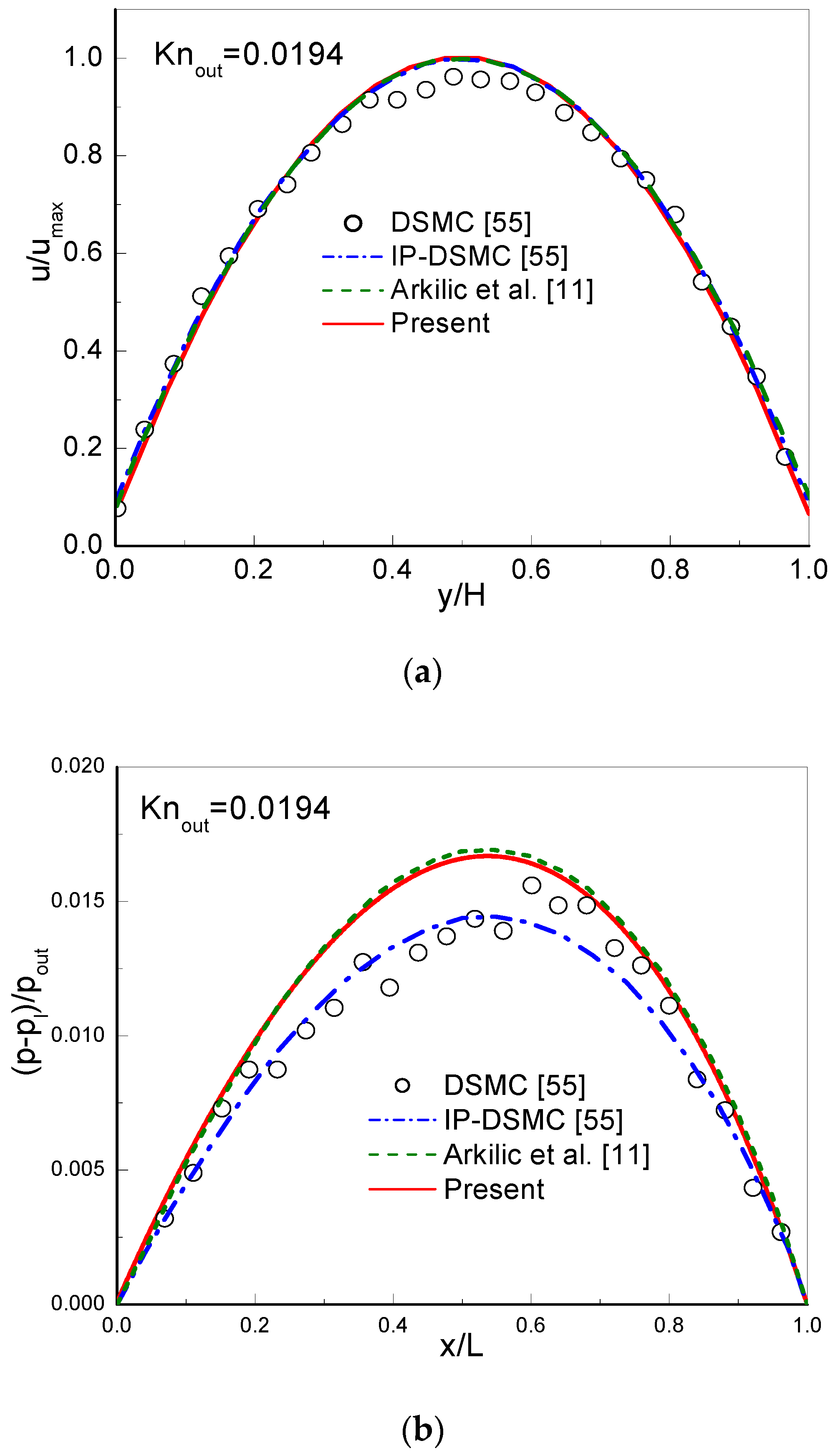
3.2. Microchannel Gas Flow with Pressure Boundary Condition

In this subsection, the microchannel gas flow with pressure boundary conditions [54,55] is studied by the CLB method. In this problem, a 2D microchannel with height $H$ and length $L$ is considered. The pressures at the inlet and outlet are $p_{\mathrm{in}}$ and $p_{\mathrm{out}}$, respectively, and the flow is driven by the substantial pressure drops. Following the literature [55], $L/H$ is set to $100$. The local Knudsen number $Kn$ is determined by $Kn=K{n}_{\mathrm{out}}{p}_{\mathrm{out}}/p\left(x\right)$, where $p\left(x\right)$ is the local pressure along the centerline, and $K{n}_{\mathrm{out}}$ is the Knudsen number at the outlet.

In simulations, a uniform lattice $N_x\times N_y=2000\times 20$ is employed. The CBBSR boundary scheme is applied at the bottom and top walls, and the pressure boundary conditions at the inlet and outlet are realized by the consistent linear extrapolation scheme developed by Verhaeghe et al. [30]. We first consider the following three cases with $\sigma =1$: (i) $K{n}_{\mathrm{out}}=0.0194$, $p_{\mathrm{in}}/p_{\mathrm{out}}=1.4$; (ii) $K{n}_{\mathrm{out}}=0.194$, $p_{\mathrm{in}}/p_{\mathrm{out}}=2$; (iii) $K{n}_{\mathrm{out}}=0.388$, $p_{\mathrm{in}}/p_{\mathrm{out}}=2$. The dimensionless streamwise velocity ${u_x/u}_{x,\max }$ at the outlet and the pressure deviation $\delta p=\left(p-p_l\right)/p_{\mathrm{out}}$ along the centerline are shown in Figure 3, Figure 4 and Figure 5. Here, $u_{x,\max }$ is the maximum streamwise velocity, and $p_l=p_{\mathrm{in}}+\left(p_{\mathrm{in}}-p_{\mathrm{out}}\right)x/L$ is the linear distributed pressure along the centerline. The analytical solutions [11] derived from the NS equations with first-order slip boundary condition (slip NS solutions) and the DSMC and IP-DSMC results [55] are also presented in the figures for comparison. For $K{n}_{\mathrm{out}}=0.0194$ (slip flow) and $p_{\mathrm{in}}/p_{\mathrm{out}}=1.4$ (see Figure 3), the velocity profiles and pressure deviation obtained by the CLB method agree well with the slip NS solutions, but show slight discrepancy with the DSMC and IP-DSMC results. When $K{n}_{\mathrm{out}}$ increases to $0.194$ (transition flow) with $p_{\mathrm{in}}/p_{\mathrm{out}}=2.0$ (see Figure 4), the present results match the DSMC and IP-DSMC results slightly better than the NS solutions. For $K{n}_{\mathrm{out}}=0.388$ (transition flow) and $p_{\mathrm{in}}/p_{\mathrm{out}}=2$ (see Figure 5), the velocity profile of the CLB method consistent with the DSMC and IP-DSMC results, and there is little difference in the pressure deviation. However, for pressure deviation profile, the slip NS solutions obviously deviate from the DSMC and IP-DSMC results. From Figure 4 and Figure 5 we can observe that, the variation of the pressure deviation distribution from $K{n}_{\mathrm{out}}=0.194$ to ${\mathrm{Kn}}_{\mathrm{out}}=0.388$ ($p_{\mathrm{in}}/p_{\mathrm{out}}=2$) decreases as the rarefaction effect increases.

The streamwise velocity ($U$) and the spanwise velocity ($V$) for $K{n}_{\mathrm{out}}=0.194$ and $p_{\mathrm{in}}/p_{\mathrm{out}}=2$ are presented in Figure 6. The streamwise and spanwise velocities are normalized by $u_{x,\max }$, i.e., $U=u_x/u_{x,\max }$ and $V=u_y/u_{x,\max }$. Figure 6a shows the phenomenon of velocity slip at the bottom and top walls, and along the microchannel, it is observed that the slip velocity increases. As shown in Figure 6b, the spanwise velocity’s magnitude is substantially smaller than that of the streamwise velocity, and the spanwise velocity distribution clearly indicates that as the flow progresses down the microchannel, it migrates from the centerline towards the wall. The above observations agree well with those reported in [25,31].

In what follows, the rarefaction effects on mass flow rate are studied. In order to make comparisons with the experimental results of Helium flows [12,13,14], the pressure ratio $p_{\mathrm{in}}/p_{\mathrm{out}}$ and $\sigma$ are set to $1.8$ and $0.93$, respectively. The dimensionless mass flow rate is $S=m/m_{\mathrm{ns}}$, where $m={\displaystyle {\int }_0^H\left(\rho u_x\right)}dy$ is the mass flow rate, and $m_{\mathrm{ns}}$ is the corresponding mass flow rate without rarefaction effect (continuum flow). In Colin et al.’s experimental work [13,14], the inverse dimensionless mass flow rate ($1/S$) was plotted against $K{n}_{\mathrm{out}}$ for Helium flows in a long microchannel up to $K{n}_{\mathrm{out}}=0.47$. In the experiment study of Maurer et al. [12], dimensionless mass flow rate ($S$) was plotted against $K{n}_{\mathrm{ave}}=\left(K{n}_{\mathrm{in}}+K{n}_{\mathrm{out}}\right)/2$ for Helium flows in a long microchannel up to $K{n}_{\mathrm{ave}}\approx 0.8$. In Figure 7a,b, the inverse dimensionless mass flow rate $1/S$ and the dimensionless mass flow rate $S$ are plotted against $K{n}_{\mathrm{out}}$ and $K{n}_{\mathrm{ave}}$, respectively. The analytical solutions of Aubert and Colin [7] and Arkilic et al. [11] are also presented in Figure 7 for comparison. From Figure 7a we can observe that, Aubert and Colin’s second-order slip model and the present CLB method predict nearly the same mass flow rate up to $K{n}_{\mathrm{out}}=0.15$. As $K{n}_{\mathrm{out}}$ increases, Aubert and Colin’s analytical solutions gradually deviate from the experimental data, while the present results are consistent with the experimental predictions up to $K{n}_{\mathrm{out}}=0.5$. A similar phenomenon can also be observed in Figure 7b. The above comparisons indicate that by using the Bosanquet-type effective viscosity with the CBBSR boundary scheme, the present CLB method is able to accurately capture the characteristic flow behaviors of pressure-driven gas flow in a long microchannel in the transition flow regime with moderate Knudsen numbers.

4. Conclusions

A CLB method is developed for studying microchannel gas flows in the transition flow regime. In the CLB method, the Bosanquet-type effective viscosity is employed to capture the rarefaction effects, and accordingly the CBBSR boundary scheme with a modified second-order slip boundary condition is employed. Numerical simulations are carried out for the microchannel gas flow with periodic and pressure boundary conditions from the slip flow regime to the transition flow regime. The predicted results agree well with the results reported in previous studies. For the microchannel gas flow with periodic boundary condition, the Knudsen minimum phenomenon is captured by the CLB method at $Kn\approx 0.9$ (the dimensionless flow rate $Q=1.6550$). For the microchannel gas flow with pressure boundary conditions, the distributions of the streamwise and spanwise velocities, and the rarefaction effects on mass flow rate, are well captured by the CLB method. The present CLB method can serve as an efficient numerical tool for studying microchannel rarefied gas flows from the slip flow to the transition flow regime.

References

1. Ho, C.M.; Tai, Y.C. Micro-electro-mechanical-systems (MEMS) and fluid flows. Annu. Rev. Fluid Mech. 1998, 30, 579–612. [Google Scholar] [CrossRef] [Green Version]
2. Karniadakis, G.E.; Beskok, A. Micro Flows: Fundamentals and Simulation; Springer: New York, NY, USA, 2002. [Google Scholar]
3. Barber, R.W.; Emerson, D.R. Challenges in modeling gas-phase flow in microchannels: From slip to transition. Heat Transf. Eng. 2006, 27, 3–12. [Google Scholar] [CrossRef]
4. Zhang, W.-M.; Meng, G.; Wei, X. A review on slip models for gas microflows. Microfluid. Nanofluid. 2012, 13, 845–882. [Google Scholar] [CrossRef]
5. Tsien, H.-S. Superaerodynamics, Mechanics of Rarefied Gases. J. Aeronaut. Sci. 1946, 13, 653–664. [Google Scholar] [CrossRef]
6. Gad-El-Hak, M. The Fluid Mechanics of Microdevices—The Freeman Scholar Lecture. J. Fluids Eng. 1999, 121, 5–33. [Google Scholar] [CrossRef]
7. Aubert, C.; Colin, S. High-order boundary conditions for gaseous flows in rectangular microducts. Microscale Thermophys. Eng. 2001, 5, 41–54. [Google Scholar]
8. Cercignani, C. Mathematical Methods in Kinetic Theory; Plenum Press: New York, NY, USA, 1990. [Google Scholar]
9. Cercignani, C.; Lampis, M.; Lorenzani, S. Variational approach to gas flows in microchannels. Phys. Fluids 2004, 16, 3426–3437. [Google Scholar] [CrossRef]
10. Schaaf, S.A.; Chambré, P.L. Flow of Rarefied Gases; Princeton University Press: Princeton, NJ, USA, 1961. [Google Scholar]
11. Arkilic, E.; Schmidt, M.; Breuer, K. Gaseous slip flow in long microchannels. J. Microelectromech. Syst. 1997, 6, 167–178. [Google Scholar] [CrossRef] [Green Version]
12. Maurer, J.; Joseph, P.; Tabeling, P.; Willaime, H. Second-order slip laws in microchannels for helium and nitrogen. Phys. Fluids 2003, 15, 2613–2621. [Google Scholar] [CrossRef]
13. Colin, S.; LaLonde, P.; Caen, R. Validation of a Second-Order Slip Flow Model in Rectangular Microchannels. Heat Transf. Eng. 2004, 25, 23–30. [Google Scholar] [CrossRef] [Green Version]
14. Colin, S. Rarefaction and compressibility effects on steady and transient gas flows in microchannels. Microfluid. Nanofluid. 2005, 1, 268–279. [Google Scholar] [CrossRef]
15. Bird, G.A. Molecular Gas Dynamics and the Direct Simulation of Gas Flows; Clarendon Press: Oxford, UK, 1994. [Google Scholar]
16. Sharipov, F. Non-isothermal gas flow through rectangular microchannels. J. Micromech. Microeng. 1999, 9, 394–401. [Google Scholar] [CrossRef]
17. Naris, S.; Valougeorgis, D.; Sharipov, F.; Kalempa, D. Discrete velocity modelling of gaseous mixture flows in MEMS. Superlattice. Microst. 2004, 35, 629–643. [Google Scholar] [CrossRef]
18. Nie, X.; Doolen, G.D.; Chen, S. Lattice-Boltzmann Simulations of Fluid Flows in MEMS. J. Stat. Phys. 2002, 107, 279–289. [Google Scholar] [CrossRef]
19. Lim, C.Y.; Niu, X.D.; Shu, C.; Chew, Y.T. Application of lattice Boltzmann method to simulate microchannel flows. Phys. Fluids 2002, 14, 2299–2308. [Google Scholar] [CrossRef]
20. Xu, K.; Li, Z. Microchannel flow in the slip regime: Gas-kinetic BGK–Burnett solutions. J. Fluid Mech. 2004, 513, 87–110. [Google Scholar] [CrossRef]
21. Guo, Z.; Xu, K.; Wang, R. Discrete unified gas kinetic scheme for all Knudsen number flows: Low-speed isothermal case. Phys. Rev. E 2013, 88, 033305. [Google Scholar] [CrossRef] [Green Version]
22. Succi, S. Mesoscopic Modeling of Slip Motion at Fluid-Solid Interfaces with Heterogeneous Catalysis. Phys. Rev. Lett. 2002, 89, 064502. [Google Scholar] [CrossRef]
23. Ansumali, S.; Karlin, I.V. Kinetic boundary conditions in the lattice Boltzmann method. Phys. Rev. E 2002, 66, 026311. [Google Scholar] [CrossRef] [Green Version]
24. Tang, G.H.; Tao, W.Q.; He, Y.L. Lattice Boltzmann Method for Simulating Gas Flow in Microchannels. Int. J. Mod. Phys. C 2004, 15, 335–347. [Google Scholar] [CrossRef] [Green Version]
25. Guo, Z.; Zhao, T.S.; Shi, Y. Physical symmetry, spatial accuracy, and relaxation time of the lattice Boltzmann equation for microgas flows. J. Appl. Phys. 2006, 99, 074903. [Google Scholar] [CrossRef]
26. Tang, G.H.; Tao, W.Q.; He, Y.L. Simulating two- and three-dimensional microflows by the lattice boltzmann method with kinetic boundary conditions. Int. J. Mod. Phys. C 2007, 18, 805–817. [Google Scholar] [CrossRef] [Green Version]
27. Guo, Z.; Zheng, C.; Shi, B. Lattice Boltzmann equation with multiple effective relaxation times for gaseous microscale flow. Phys. Rev. E 2008, 77, 036707. [Google Scholar] [CrossRef] [PubMed]
28. Kim, S.H.; Pitsch, H.; Boyd, I.D. Accuracy of higher-order lattice Boltzmann methods for microscale flows with finite Knudsen numbers. J. Comput. Phys. 2008, 227, 8655–8671. [Google Scholar] [CrossRef]
29. Tang, G.H.; Zhang, Y.H.; Gu, X.J.; Emerson, D.R. Lattice Boltzmann modelling Knudsen layer effect in non-equilibrium flows. Europhys. Lett. 2008, 83, 40008–40014. [Google Scholar] [CrossRef] [Green Version]
30. Verhaeghe, F.; Luo, L.-S.; Blanpain, B. Lattice Boltzmann modeling of microchannel flow in slip flow regime. J. Comput. Phys. 2009, 228, 147–157. [Google Scholar] [CrossRef]
31. Li, Q.; He, Y.L.; Tang, G.H.; Tao, W.Q. Lattice Boltzmann modeling of microchannel flows in the transition flow regime. Microfluid. Nanofluid. 2011, 10, 607–618. [Google Scholar] [CrossRef]
32. Zhuo, C.; Zhong, C. Filter-matrix lattice Boltzmann model for microchannel gas flows. Phys. Rev. E 2013, 88, 053311. [Google Scholar] [CrossRef]
33. Chen, L.; Zhang, L.; Kang, Q.; Viswanathan, H.S.; Yao, J.; Tao, W. Nanoscale simulation of shale transport properties using the lattice Boltzmann method: Permeability and diffusivity. Sci. Rep. 2015, 5, 8089. [Google Scholar] [CrossRef]
34. Chen, S.; Doolen, G.D. Lattice Boltzmann method for fluid flows. Annu. Rev. Fluid Mech. 1998, 30, 329–364. [Google Scholar] [CrossRef] [Green Version]
35. Succi, S. The Lattice Boltzmann Equation: For Fluid Dynamics and Beyond; Oxford University Press: Oxford, UK, 2001. [Google Scholar]
36. Succi, S. Lattice Boltzmann across scales: From turbulence to DNA translocation. Eur. Phys. J. B 2008, 64, 471–479. [Google Scholar] [CrossRef]
37. Xu, A.; Shi, L.; Xi, H.D. Lattice Boltzmann simulations of three-dimensional thermal convective flows at high Rayleigh number. Int. J. Heat Mass Transfer 2019, 140, 359–370. [Google Scholar] [CrossRef] [Green Version]
38. Zhang, J. Lattice Boltzmann method for microfluidics: Models and applications. Microfluid. Nanofluid. 2011, 10, 1–28. [Google Scholar] [CrossRef]
39. Li, Q.; Luo, K.H.; Kang, Q.J.; He, Y.L.; Chen, Q.; Liu, Q. Lattice Boltzmann methods for multiphase flow and phase-change heat transfer. Prog. Energy Combust. Sci. 2016, 52, 62–105. [Google Scholar] [CrossRef] [Green Version]
40. Xu, A.; Shyy, W.; Zhao, T. Lattice Boltzmann modeling of transport phenomena in fuel cells and flow batteries. Acta Mech. Sin. 2017, 33, 555–574. [Google Scholar] [CrossRef]
41. Frisch, U.; Hasslacher, B.; Pomeau, Y. Lattice-Gas Automata for the Navier-Stokes Equation. Phys. Rev. Lett. 1986, 56, 1505–1508. [Google Scholar] [CrossRef] [Green Version]
42. Geier, M.; Greiner, A.; Korvink, J.G. Cascaded digital lattice Boltzmann automata for high Reynolds number flow. Phys. Rev. E 2006, 73, 066705. [Google Scholar] [CrossRef]
43. Premnath, K.N.; Banerjee, S. Incorporating forcing terms in cascaded lattice Boltzmann approach by method of central moments. Phys. Rev. E 2009, 80, 036702. [Google Scholar] [CrossRef] [Green Version]
44. Geller, S.; Uphoff, S.; Krafczyk, M. Turbulent jet computations based on MRT and Cascaded Lattice Boltzmann models. Comput. Math. Appl. 2013, 65, 1956–1966. [Google Scholar] [CrossRef]
45. Lycett-Brown, D.; Luo, K.H. Multiphase cascaded lattice Boltzmann method. Comput. Math. Appl. 2014, 67, 350–362. [Google Scholar] [CrossRef] [Green Version]
46. LeClaire, S.; Pellerin, N.; Reggio, M.; Trépanier, J.-Y. Multiphase flow modeling of spinodal decomposition based on the cascaded lattice Boltzmann method. Phys. A Stat. Mech. Appl. 2014, 406, 307–319. [Google Scholar] [CrossRef]
47. Lallemand, P.; Luo, L.-S. Theory of the lattice Boltzmann method: Dispersion, dissipation, isotropy, Galilean invariance, and stability. Phys. Rev. E 2000, 61, 6546–6562. [Google Scholar] [CrossRef] [PubMed] [Green Version]
48. Asinari, P. Generalized local equilibrium in the cascaded lattice Boltzmann method. Phys. Rev. E 2008, 78, 016701. [Google Scholar] [CrossRef] [PubMed] [Green Version]
49. Qian, Y.H.; d’Humières, D.; Lallemand, P. Lattice BGK models for Navier-Stokes equation. Europhys. Lett. 1992, 17, 479–484. [Google Scholar] [CrossRef]
50. Beskok, A.; Karniadakis, G.E. A model for flows in channels, pipes, and ducts at micro and nano scales. Microscale Thermophys. Eng. 1999, 3, 43–77. [Google Scholar]
51. Michalis, V.K.; Kalarakis, A.N.; Skouras, E.D.; Burganos, V.N. Rarefaction effects on gas viscosity in the Knudsen transition regime. Microfluid. Nanofluid. 2010, 9, 847–853. [Google Scholar] [CrossRef]
52. Ohwada, T.; Sone, Y.; Aoki, K. Numerical analysis of the Poiseuille and thermal transpiration flows between two parallel plates on the basis of the Boltzmann equation for hard-sphere molecules. Phys. Fluids A Fluid Dyn. 1989, 1, 2042–2049. [Google Scholar] [CrossRef]
53. Hadjiconstantinou, N.G. Comment on Cercignani’s second-order slip coefficient. Phys. Fluids 2003, 15, 2352–2354. [Google Scholar] [CrossRef] [Green Version]
54. Dongari, N.; Sharma, A.; Durst, F. Pressure-driven diffusive gas flows in micro-channels: From the Knudsen to the continuum regimes. Microfluid. Nanofluid. 2009, 6, 679–692. [Google Scholar] [CrossRef]
55. Shen, C.; Tian, D.B.; Xie, C.; Fan, J. Examination of the LBM in simulation of microchannel flow in transitional regime. Microscale Thermophys. Eng. 2004, 8, 423–432. [Google Scholar] [CrossRef] [Green Version]
Figure 1. Dimensionless velocity profiles at K n = 2 k / π with k ranging from 0.1 to 10 .
Entropy 22 00041 g001aEntropy 22 00041 g001b
Figure 2. Dimensionless flow rate against the Knudsen number K n .
Entropy 22 00041 g002
Figure 3. Streamwise velocity at the outlet (a) and pressure deviation along the channel centerline (b) for K n out = 0.0194 and p in / p out = 1.4 .
Entropy 22 00041 g003
Figure 4. Streamwise velocity at the outlet (a) and pressure deviation along the channel centerline (b) for K n out = 0.194 and p in / p out = 2 .
Entropy 22 00041 g004aEntropy 22 00041 g004b
Figure 5. Streamwise velocity at the outlet (a) and pressure deviation along the channel centerline (b) for K n out = 0.388 and p in / p out = 2 .
Entropy 22 00041 g005aEntropy 22 00041 g005b
Figure 6. Streamwise (a) and spanwise (b) velocities for K n out = 0.194 and p in / p out = 2 .
Entropy 22 00041 g006aEntropy 22 00041 g006b
Figure 7. The inverse dimensionless mass flow rate 1 / S (a) and the dimensionless mass flow rate S (b) for σ = 0.93 and p in / p out = 1.8 .
Entropy 22 00041 g007aEntropy 22 00041 g007b