Quantum Adiabatic Pumping in Rashba- Dresselhaus-Aharonov-Bohm Interferometer

Abstract

We investigate the quantum adiabatic pumping effect in an interferometer attached to two one-dimensional leads. The interferometer is subjected to an Aharonov-Bohm flux and Rashba-Dresselhaus spin-orbit interaction. Using Brouwer’s formula and rigorous scattering eigenstates, we obtained the general closed formula for the pumping Berry curvatures depending on spin for general interferometers when the external control parameters only modulate the scattering eigenstates and corresponding eigenvalues. In this situation, pumping effect is absent in the combination of the control parameters of Aharonov-Bohm flux and spin-orbit interaction strength. We have shown that finite pumping is possible by modulating both Rashba and Dresselhaus interaction strengths and explicitly demonstrated the spin-pumping effect in a diamond-shaped interferometer made of four sites.

1. Introduction

Coherent transport in mesoscopic systems is of fundamental interest since it allows realization of various phenomena observed in quantum optics in a solid-state system. Furthermore, the electron spin degree of freedom adds an intriguing knob for the manipulation and observation of the transport phenomena. Spin-orbit interaction (SOI) effect [1] is one of the key ingredients in narrow-gap semiconductor devices, whose strength can be controlled by external gates [2], in principle, without changing the electron density. Introducing the effect of SOI to the electron interferometer structure is quite attractive since it enables perfect spin filtering effect [3,4,5]. Moreover, transient behavior in such an interferometer has been investigated [6].

In addition to passive functional devices such as filters, the active functions, for example, spin-pumping or spin manipulation effect by dynamically modulating the gate voltages [7,8,9], magnetic field [10,11,12,13], or magnetization of the ferromagnets [14,15,16,17], has been investigated. In particular, quantum adiabatic pumping (QAP) phenomena [18,19], which stems from geometrical properties of the dynamics, is an active field of research [20,21,22,23,24,25]. In the non-interacting limit, QAP is related to the scattering matrix of the coherent transport. We have investigated the QAP effect by adiabatically modulating the Aharonov-Bohm (AB) phase [26] of the interferometer as well as the local potential in the interferometer. However, it seems no studies have been made of the adiabatic spin-pumping with purely geometric means such as Aharonov-Casher phase or AB phase. The fundamental question here is whether QAP is possible by only modulating the electron geometric phase.

In this work, we studied spin-QAP in Rashba-Dresselhaus-Aharonov-Bohm interferometer introduced in [3] using Brouwer’s formula [19] and derived an explicit formula of the Berry curvature for each spin component. Using the obtained result, we clarified the condition of finite spin-pumping. In Section 2, we introduce a simple two-terminal setup and the expressions of the scattering amplitudes. Section 3 explains the details of the eigenstates of the scattering problem. Then, with these states, the formula of the QAP is derived in Section 4. It is shown that the modulation of the AB phase cannot induce QAP. Section 5 explains the properties of the diamond-shape interferometer, and is applied to study QAP assuming Rashba SOI and Dresselhaus SOI strengths as control parameters in Section 6. Finally, discussions follow in Section 7 and Appendices are included for the detailed derivations of the formula used in the main text.

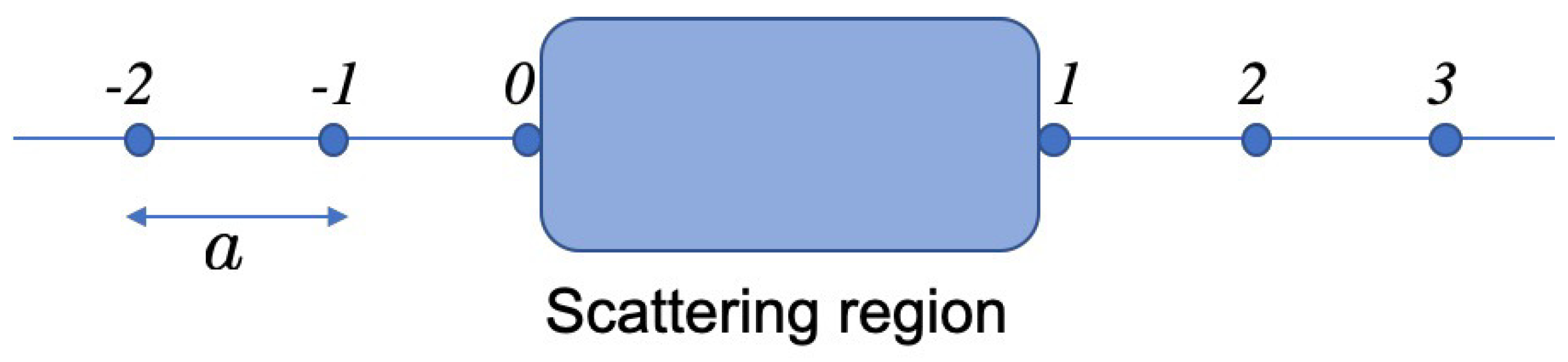
We consider a standard setup of scattering problem of spin $1/2$ electrons as shown in Figure 1. A coherent scattering region (interferometer) is attached at the site $u=0$ with the one-dimensional left lead made of sites $u=-1,-2,\dots$ and is attached at the site $u=1$ with the one-dimensional right lead made of sites $u=2,3,\dots$. The assumption of one-dimensional leads is not essential as far as the interferometer is coupled to the leads via single mode scattering channels. However, the one-dimensional tight-binding formalism benefits from its simplicity. Although the analysis is standard, the obtained rigorous scattering amplitudes and corresponding scattering eigenstates are essential to clarify the condition and to quantify the quantum adiabatic spin-pumping, as will be shown in the later sections. We introduce the spinor ket vector at site u,

$$\begin{array}{ccc}\hfill |\psi \left(u\right)⟩& \equiv & \left(\begin{array}{c}{c}_{u\uparrow }\\ c_{u\downarrow }\end{array}\right),\hfill \end{array}$$

(1)

where the two amplitudes $c_{u\sigma }$ for spin $\sigma =\uparrow ,\downarrow$ satisfy normalization condition ${\left|c_{u\uparrow }\right|}^2+{\left|c_{u\downarrow }\right|}^2=1$. The total Hamiltonian in the tight-binding approximation is given in general

$$\begin{array}{ccc}\hfill {\widehat{\mathcal{H}}}_{\mathrm{TB}}& \equiv & {\displaystyle \sum _u}{ϵ}_u|\psi \left(u\right)⟩⟨\psi \left(u\right)|+{\displaystyle \sum _{uv}}{\widehat{W}}_{uv}|\psi \left(v\right)⟩⟨\psi \left(u\right)|,\hfill \end{array}$$

(2)

where the site index u and v run the entire system. The real parameter ${ϵ}_u$ is spin-degenerate site energy and ${\widehat{W}}_{uv}$ is a $2\times 2$ hopping matrix satisfying ${\widehat{W}}_{uv}^{†}={\widehat{W}}_{vu}$. We assume that the hopping matrix ${\widehat{W}}_{uv}$ is only non-diagonal in the scattering region between $u=0$ and $u=1$. We neglect the electron-electron interaction.

Figure 1. Schematics of the model of a scattering (shaded) region connected with two semi-infinite one-dimensional leads.

2. Model System

In the leads $u\le -1$, $u\ge 2$, we set ${ϵ}_u=0$ and ${\widehat{W}}_{uv}=-j\mathbb{I}$, where $\mathbb{I}$ is the two-dimensional unit matrix and the real hopping parameter j is only nonzero for nearest-neighbor pair of $u,v$. With a standard treatment on the tight-binding Hamiltonian, we obtain the eigen-energy ${ϵ}_k\equiv -2jcos\left(ka\right)$ and its corresponding eigen-function, $|\psi \left(u\right)⟩\propto e^{ikau}|\chi ⟩$, where k is a real wave-number parameter, $a(>0)$ is the lattice constant and $|\chi ⟩$ is a certain state vector.

The system of interferometer is represented between $u=0$ and $u=1$ sites and we choose ${ϵ}_0=y_0$ and ${ϵ}_1=y_1$ and ${\widehat{W}}_{01}\equiv \widehat{W}$ and ${\widehat{W}}_{10}={\widehat{W}}^{†}$. The microscopic derivations of $y_0,y_1$ and $\widehat{W}$ for a diamond-shaped interferometer are demonstrated in Section 5. Then the Schrödinger equations at sites $u=0,1$ read

$$\begin{array}{ccc}\hfill y_0|\psi \left(0\right)⟩+\widehat{W}|\psi \left(1\right)⟩-j|\psi (-1)⟩& =& ϵ|\psi \left(0\right)⟩,\hfill \end{array}$$

(3)

$$\begin{array}{ccc}\hfill y_1|\psi \left(1\right)⟩+{\widehat{W}}^{†}|\psi \left(0\right)⟩-j|\psi \left(2\right)⟩& =& ϵ|\psi \left(1\right)⟩.\hfill \end{array}$$

(4)

The reflection and transmission amplitude matrices for the electron flux with an energy $ϵ={ϵ}_k$ injected from the left lead is

$$\begin{array}{ccc}\hfill \widehat{r}& =& -\mathbb{I}+i{\eta }_k{X}_1{\left[\mathbb{I}Y-\widehat{W}{\widehat{W}}^{†}\right]}^{-1},\hfill \end{array}$$

(5)

$$\begin{array}{ccc}\hfill \widehat{t}& =& i{\eta }_k{\widehat{W}}^{†}{\left[\mathbb{I}Y-\widehat{W}{\widehat{W}}^{†}\right]}^{-1},\hfill \end{array}$$

(6)

where $Y\equiv X_0{X}_1$ with complex parameters $X_u\equiv {ϵ}_k-y_u+j{e}^{ika}$ ($u=0,1$) and we introduced a parameter of energy dimension ${\eta }_k\equiv 2jsin\left(ka\right)$. The reflection and transmission amplitude matrices for the electron flux injected from the right lead is

$$\begin{array}{ccc}\hfill {\widehat{r}}^{\prime }& =& -\mathbb{I}+i{\eta }_k{X}_0{\left[\mathbb{I}Y-{\widehat{W}}^{†}\widehat{W}\right]}^{-1},\hfill \end{array}$$

(7)

$$\begin{array}{ccc}\hfill {\widehat{t}}^{\prime }& =& i{\eta }_k\widehat{W}{\left[\mathbb{I}Y-{\widehat{W}}^{†}\widehat{W}\right]}^{-1}.\hfill \end{array}$$

(8)

The details of the derivation of these formulae are given in Appendix A. In the next section, the obtained scattering amplitude matrices are diagonalized and the formulae of the scattering amplitude eigenvalues are given. Then in Section 4, the Berry curvatures for two spin eigenstates, Equations (34) and (35), is given, which allow calculation of QAP spin per cycle.

3. Diagonalization of Hopping Operator $\widehat{\mathit{W}}{\widehat{\mathit{W}}}^{†}$

In this section, we diagonalize the product of hopping operators $\widehat{W}$ and ${\widehat{W}}^{†}$ appearing in the scattering amplitude matrices derived in the previous section. Then we obtain the scattering eigenstates through an interferometer. This is an extension of the discussion in Reference [3]. We consider an interferometer in $x-y$ plane made of two one-dimensional arms, b and c, represented by real coupling parameters ${\gamma }_b,{\gamma }_c$ and $2\times 2$ unitary matrices, ${\widehat{U}}_b$ and ${\widehat{U}}_c$, showing propagation from the site 0 to 1 via the arms b and c, respectively. We assume following general expressions characterizing the effect of AB phase and Rashba or Dresselhaus SOI:

$$\begin{array}{ccc}\hfill {\widehat{U}}_b& =& e^{-i{\varphi }_1}\left(\mathbb{I}\delta +i\mathit{\tau }·\widehat{\mathit{\sigma }}\right),\hfill \end{array}$$

(9)

$$\begin{array}{ccc}\hfill {\widehat{U}}_c& =& e^{i{\varphi }_2}\left(\mathbb{I}{\delta }^{\prime }+i{\mathit{\tau }}^{\prime }·\widehat{\mathit{\sigma }}\right),\hfill \end{array}$$

(10)

where $\widehat{\mathit{\sigma }}$ is the vector of Pauli spin matrices. $\varphi \equiv {\varphi }_1+{\varphi }_2=2\pi \left(HS\right)/{\mathsf{\Phi }}_0$ is the AB phase with the magnetic field H in the z direction, the area of the interferometer S, and a magnetic flux quantum ${\mathsf{\Phi }}_0$. Unitarity condition requires the real parameters, $\delta ,{\delta }^{\prime }$ and real three-dimensional vectors $\mathit{\tau },{\mathit{\tau }}^{\prime }$ to obey ${\delta }^2+{\left|\mathit{\tau }\right|}^2={\delta }^{\prime 2}+{\left|{\mathit{\tau }}^{\prime }\right|}^2=1$. The hopping matrix $\widehat{W}$ is given by

$$\begin{array}{ccc}\hfill \widehat{W}& =& {\gamma }_b{\widehat{U}}_b+{\gamma }_c{\widehat{U}}_c.\hfill \end{array}$$

(11)

As shown in Appendix B, the matrix factor appearing in the scattering amplitudes for the electron flux injected from the left lead, Equation (5), is

$$\begin{array}{ccc}\hfill \widehat{W}{\widehat{W}}^{†}& \equiv & A\mathbb{I}+\mathit{B}·\widehat{\mathit{\sigma }},\hfill \end{array}$$

(12)

where

$$\begin{array}{ccc}\hfill A& =& {\gamma }_b^2+{\gamma }_c^2+2{\gamma }_b{\gamma }_{c}cos\varphi cos\omega ,\hfill \end{array}$$

(13)

$$\begin{array}{ccc}\hfill \mathit{B}& =& 2{\gamma }_b{\gamma }_{c}sin\varphi sin\omega \widehat{\mathit{n}}.\hfill \end{array}$$

(14)

The real parameter $\omega$ is determined from $cos\omega \equiv \delta {\delta }^{\prime }+\mathit{\tau }·{\mathit{\tau }}^{\prime }$ and the unit vector $\widehat{\mathit{n}}$ is defined by

$$\begin{array}{ccc}\hfill \widehat{\mathit{n}}& =& \frac{1}{\sqrt{1-{\tau }_z^2}}(-{\tau }_y,{\tau }_x,\delta ).\hfill \end{array}$$

(15)

We then introduce two normalized eigenstates of the operator $\widehat{\mathit{n}}·\widehat{\mathit{\sigma }}$, $|\widehat{\mathit{n}}⟩$ and $|-\widehat{\mathit{n}}⟩$ such that

$$\begin{array}{ccc}\hfill \widehat{\mathit{n}}·\widehat{\mathit{\sigma }}|\widehat{\mathit{n}}⟩& =& |\widehat{\mathit{n}}⟩,\hfill \end{array}$$

(16)

$$\begin{array}{ccc}\hfill \widehat{\mathit{n}}·\widehat{\mathit{\sigma }}|-\widehat{\mathit{n}}⟩& =& -|-\widehat{\mathit{n}}⟩.\hfill \end{array}$$

(17)

Clearly, these are also the eigenstates of the operator $\widehat{W}{\widehat{W}}^{†}$ such that

$$\begin{array}{ccc}\hfill \widehat{W}{\widehat{W}}^{†}|\pm \widehat{\mathit{n}}⟩& =& {\lambda }_{\pm }|\pm \widehat{\mathit{n}}⟩,\hfill \end{array}$$

(18)

with the eigenvalues

$$\begin{array}{ccc}\hfill {\lambda }_{\pm }& =& {\gamma }_b^2+{\gamma }_c^2+2{\gamma }_b{\gamma }_{c}cos(\varphi \mp \omega ).\hfill \end{array}$$

(19)

These eigenvalues are positive since ${\lambda }_{\pm }=⟨\pm \widehat{\mathit{n}}|\widehat{W}{\widehat{W}}^{†}|\pm \widehat{\mathit{n}}⟩={\left|\left|{\widehat{W}}^{†}|\pm \widehat{\mathit{n}}⟩\right|\right|}^2\ge 0.$

To study the scattering eigenstates for the electron flux injected from the right, Equation (7), we evaluate ${\widehat{W}}^{†}\widehat{W}$ with similar procedure as above,

$$\begin{array}{ccc}\hfill {\widehat{W}}^{†}\widehat{W}& \equiv & A\mathbb{I}+{\mathit{B}}^{\prime }·\widehat{\mathit{\sigma }},\hfill \end{array}$$

(20)

where

$$\begin{array}{ccc}\hfill {\mathit{B}}^{\prime }& =& 2{\gamma }_b{\gamma }_{c}sin\varphi sin\omega {\widehat{\mathit{n}}}^{\prime },\hfill \end{array}$$

(21)

and corresponding unit vector

$$\begin{array}{ccc}\hfill {\widehat{\mathit{n}}}^{\prime }& =& \frac{1}{\sqrt{1-{\tau }_z^2}}({\tau }_y,-{\tau }_x,\delta ).\hfill \end{array}$$

(22)

Then we introduce two normalized eigenstates of the operator ${\widehat{\mathit{n}}}^{\prime }·\widehat{\mathit{\sigma }}$, $|\pm {\widehat{\mathit{n}}}^{\prime }⟩$, which obey

$$\begin{array}{ccc}\hfill {\widehat{W}}^{†}\widehat{W}|\pm {\widehat{\mathit{n}}}^{\prime }⟩& =& {\lambda }_{\pm }|\pm {\widehat{\mathit{n}}}^{\prime }⟩,\hfill \end{array}$$

(23)

with the same eigenvalues as Equation (18).

The elements of the scattering matrix are now explicitly evaluated with the obtained scattering eigenstates. As detailed in Appendix B, we can show that the transmission amplitude matrices are

$$\begin{array}{ccc}\hfill \widehat{t}& =& t_{+}|{\widehat{\mathit{n}}}^{\prime }⟩⟨\widehat{\mathit{n}}|+t_{-}|-{\widehat{\mathit{n}}}^{\prime }⟩⟨-\widehat{\mathit{n}}|,\hfill \end{array}$$

(24)

$$\begin{array}{ccc}\hfill {\widehat{t}}^{\prime }& =& t_{+}|\widehat{\mathit{n}}⟩⟨{\widehat{\mathit{n}}}^{\prime }|+t_{-}|-\widehat{\mathit{n}}⟩⟨-{\widehat{\mathit{n}}}^{\prime }|,\hfill \end{array}$$

(25)

where we defined two transmission amplitudes,

$$\begin{array}{ccc}\hfill t_{\pm }& \equiv & \frac{i{\eta }_k\sqrt{{\lambda }_{\pm }}}{Y-{\lambda }_{\pm }}.\hfill \end{array}$$

(26)

Similarly, the reflection amplitude matrices are given by

$$\begin{array}{ccc}\hfill \widehat{r}& =& r_{+}|\widehat{\mathit{n}}⟩⟨\widehat{\mathit{n}}|+r_{-}|-\widehat{\mathit{n}}⟩⟨-\widehat{\mathit{n}}|,\hfill \end{array}$$

(27)

$$\begin{array}{ccc}\hfill {\widehat{r}}^{\prime }& =& r_{+}^{\prime }|{\widehat{\mathit{n}}}^{\prime }⟩⟨{\widehat{\mathit{n}}}^{\prime }|+r_{-}^{\prime }|-{\widehat{\mathit{n}}}^{\prime }⟩⟨-{\widehat{\mathit{n}}}^{\prime }|,\hfill \end{array}$$

(28)

where the reflection amplitudes are

$$\begin{array}{ccc}\hfill r_{\pm }& \equiv & -1+\frac{i{\eta }_k{X}_1}{Y-{\lambda }_{\pm }},\hfill \end{array}$$

(29)

$$\begin{array}{ccc}\hfill r_{\pm }^{\prime }& \equiv & -1+\frac{i{\eta }_k{X}_0}{Y-{\lambda }_{\pm }}.\hfill \end{array}$$

(30)

The unitarity condition of the scattering amplitude matrices, ${\widehat{t}}^{†}\widehat{t}+{\widehat{r}}^{†}\widehat{r}=1$, is confirmed in Appendix C. The unitarity condition ${\widehat{t}}^{{}^{\prime }†}{\widehat{t}}^{\prime }+{\widehat{r}}^{{}^{\prime }†}{\widehat{r}}^{\prime }=1$ can also be checked.

4. Quantum Adiabatic Pump

For a non-interacting system, the response (particle transfer) to the slow modulation of the system’s controlling parameters is well described by Brouwer’s formula [19], which is expressed by the elements of the scattering matrix. The particles induced in the left lead in one cycle of the adiabatic modulation of two control parameters $g_1$ and $g_2$ is

$$\begin{array}{ccc}\hfill n& =& {\displaystyle \sum _{\sigma }}{n}_{\sigma },\hfill \end{array}$$

(31)

$$\begin{array}{ccc}\hfill n_{\sigma }& =& -{\int }_{S}d{g}_{1}d{g}_2{\prod }_{\sigma }(g_1,g_2),\hfill \end{array}$$

(32)

where S is the area in the two-dimensional control parameter space whose edge corresponds to the trajectory of the cycle. The Berry curvature ${\prod }_{\sigma }(g_1,g_2)$ for spin $\sigma$ is

$$\begin{array}{ccc}\hfill {\prod }_{\sigma }(g_1,g_2)& =& \frac{1}{\pi }\Im ⟨\sigma |\left\{\frac{\partial \widehat{r}}{\partial g_2}\frac{\partial {\widehat{r}}^{†}}{\partial g_1}+\frac{\partial \widehat{t^{\prime }}}{\partial g_2}\frac{\partial {\widehat{t^{\prime }}}^{†}}{\partial g_1}\right\}|\sigma ⟩,\hfill \end{array}$$

(33)

where $\widehat{r}$ and ${\widehat{t}}^{\prime }$ are given in Equations (27) and (25) and $|\sigma ⟩$ is the spinor vector of spin $\sigma$.

If we choose the AB phase $\varphi$ and parameters of the interferometers, for example, $X_0$ or $X_1$, but not the SOI strengths, we can show that the Berry curvature is finite in general as studied in Reference [26]. In the following, however, we focus on the situation that the control parameters are the AB phase $\varphi$ and Rashba or Dresselhaus SOI strength that modulate the eigenvalue ${\lambda }_{\pm }$ as well as the scattering eigenstates $|\pm \widehat{\mathit{n}}⟩,|\pm {\widehat{\mathit{n}}}^{\prime }⟩$. To calculate the Berry curvature, we need to evaluate the derivatives of the scattering amplitude matrices, $\widehat{r}$ and ${\widehat{t}}^{\prime }$. Then, as shown in Appendix D, after some manipulations, we have the Berry curvatures for spin components parallel to $\pm \widehat{\mathit{n}}$,

$$\begin{array}{ccc}\hfill {\prod }_{\widehat{\mathit{n}}}(g_1,g_2)& =& \left({\left|r_{+}-r_{-}\right|}^2-{\left|t_{+}\right|}^2+{\left|t_{-}\right|}^2\right){\mathcal{C}}_{g_1,g_2},\hfill \end{array}$$

(34)

and

$$\begin{array}{ccc}\hfill {\prod }_{-\widehat{\mathit{n}}}(g_1,g_2)& =& \left(-{\left|r_{+}-r_{-}\right|}^2-{\left|t_{+}\right|}^2+{\left|t_{-}\right|}^2\right){\mathcal{C}}_{g_1,g_2}.\hfill \end{array}$$

(35)

where the factor at the end is independent of spin and is defined as

$$\begin{array}{lll}{\mathcal{C}}_{g_1,g_2}& =& \frac{1}{4\pi n_z}\frac{1}{1-{\tau }_z^2}[\frac{\partial {\tau }_y}{\partial g_1}\frac{\partial {\tau }_x}{\partial g_2}-\frac{\partial {\tau }_y}{\partial g_2}\frac{\partial {\tau }_x}{\partial g_1}\hfill \\ & +& \frac{{\tau }_z}{1-{\tau }_z^2}\left\{{\tau }_x\left(\frac{\partial {\tau }_y}{\partial g_1}\frac{\partial {\tau }_z}{\partial g_2}-\frac{\partial {\tau }_y}{\partial g_2}\frac{\partial {\tau }_z}{\partial g_1}\right)+{\tau }_y\left(\frac{\partial {\tau }_x}{\partial g_2}\frac{\partial {\tau }_z}{\partial g_1}-\frac{\partial {\tau }_x}{\partial g_1}\frac{\partial {\tau }_z}{\partial g_2}\right)\right\}].\hfill \end{array}$$

(36)

This is one of the main results of this work.

The vector $\mathit{\tau }$ is independent of $\varphi$, but only depends on the SOI strength. Therefore, when one chose the AB phase, $g_1\equiv \varphi$, as one of the control parameters, ${\mathcal{C}}_{\varphi ,g_2}$ is identically zero as is evident from Equation (36). Hence we do not expect QAP by modulating the AB phase and SOI strength. It is also obvious that if we chose ${\gamma }_b$ or ${\gamma }_c$ as one of the control parameters and the other by SOI strength, ${\mathcal{C}}_{{\gamma }_{b,c},g_2}$ is zero since $\mathit{\tau }$ is independent of ${\gamma }_b$ and ${\gamma }_c$ and no pumping is expected.

Even for a fixed AB phase, there is still some freedom to choose two control parameters related to the SOI strength since we have two types of SOI interaction mechanisms, Rashba and Dresselhaus SOI. In the next section, we study Rashba-Dresselhaus interferometer in a simple diamond-shape structure made of four sites and choose the strengths of two types of SOI as control parameters.

5. Diamond Interferometer

We consider an electron transport in two-dimensional system on $\left[001\right]$ surface with setting x and y axis along the $\left(100\right)$ and $\left(010\right)$ crystal directions, respectively. The Hamiltonian for the SOI is

$$\begin{array}{ccc}\hfill {\widehat{\mathcal{H}}}_{\mathrm{R}}& =& \frac{\hslash }{m}{k}_{\mathrm{R}}({\widehat{p}}_y{\widehat{\sigma }}_x-{\widehat{p}}_x{\widehat{\sigma }}_y),\hfill \end{array}$$

(37)

$$\begin{array}{ccc}\hfill {\widehat{\mathcal{H}}}_{\mathrm{D}}& =& \frac{\hslash }{m}{k}_{\mathrm{D}}({\widehat{p}}_x{\widehat{\sigma }}_x-{\widehat{p}}_y{\widehat{\sigma }}_y),\hfill \end{array}$$

(38)

where $k_{\mathrm{R}}$ and $k_{\mathrm{D}}$ are Rashba and Dresselhaus parameters, respectively. ${\widehat{p}}_{\mu }$ ($\mu =x,y$) are the momentum and m is the electron effective mass.

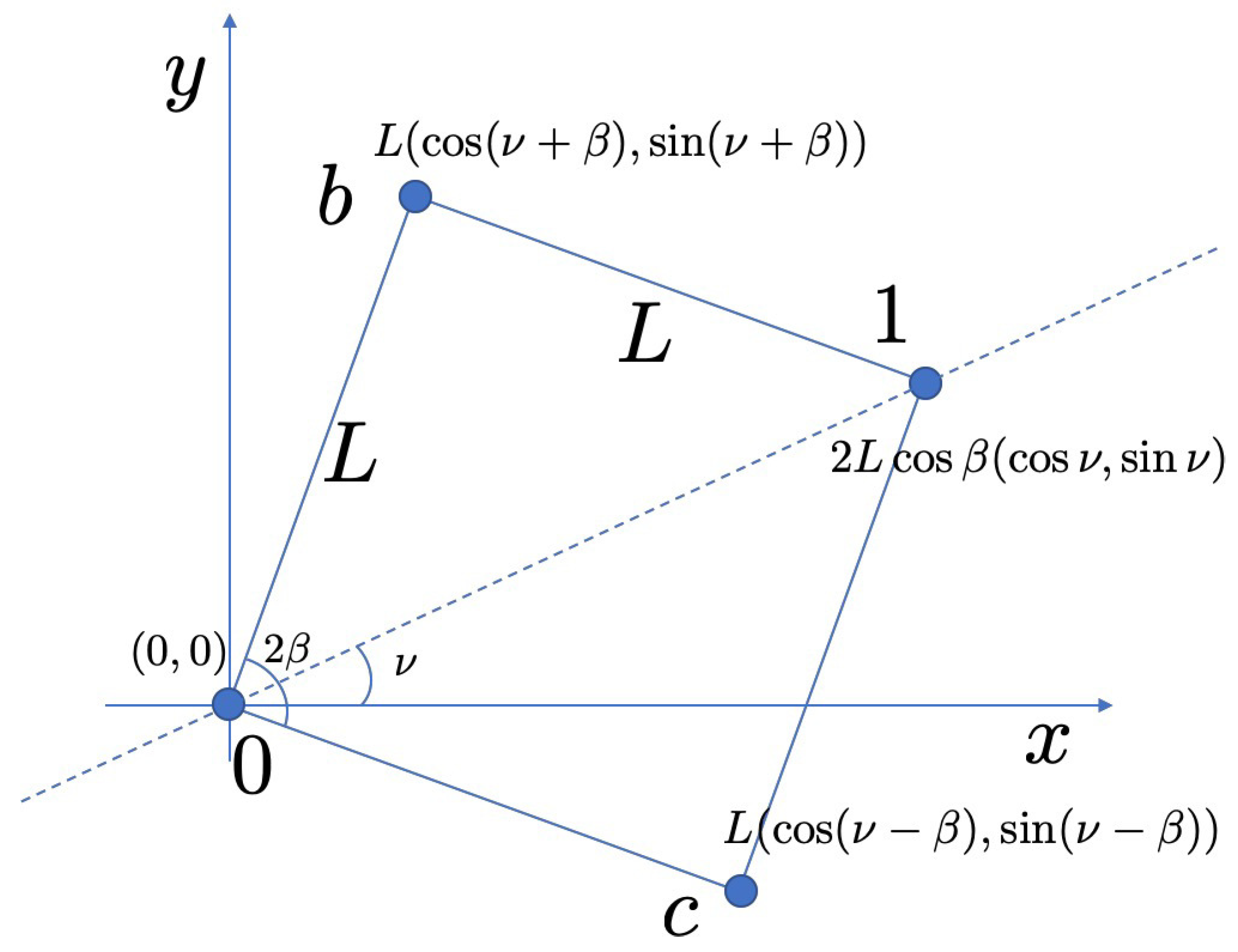
The interferometer made of four sites is configured as in Figure 2 which is attached to the leads at site $u=0$ and $u=1$ as discussed in Reference [3]. Other two sites constituting the interferometer are $u=b$ and $u=c$, connected with bonds of length L. We also define the opening angle $2\beta$ and the relative angle $\nu$ of the diagonal line to x axis. The Hamiltonian reads

$$\begin{array}{ccc}\hfill {\widehat{\mathcal{H}}}_{\mathrm{IF}}& \equiv & {\displaystyle \sum _u}{ϵ}_u|\psi \left(u\right)⟩⟨\psi \left(u\right)|-{\displaystyle \sum _{uv}}{\tilde{U}}_{uv}|\psi \left(v\right)⟩⟨\psi \left(u\right)|,\hfill \end{array}$$

(39)

for $u,v=0,c,d,1$ where ${ϵ}_u$ is the site energy and ${\tilde{U}}_{uv}\equiv J_{uv}{\widehat{U}}_{uv}$, $J_{uv}$ is a hopping energy and ${\widehat{U}}_{uv}$ is a $2\times 2$ unitary matrix representing the effect of SOI and AB phase. Total Hamiltonian is $\widehat{\mathcal{H}}={\widehat{\mathcal{H}}}_{\mathrm{IF}}+{\widehat{\mathcal{H}}}_L+{\widehat{\mathcal{H}}}_R$. In the Appendix E, we explain how this problem is reduced to the Schrödinger equations, Equations (3) and (4).

Figure 2. Schematics of the interferometer made of four sites, $0,b,c$, and 1 separated by a length L. The opening angle $2\beta$ and relative angle $\nu$ from x axis determine the geometric structure.

The coordinates of the four sites are ${\mathit{r}}_0=(0,0)$, ${\mathit{r}}_b=(Lcos(\nu +\beta ),Lsin(\nu +\beta ))$, ${\mathit{r}}_1=(2Lcos\left(\beta \right)cos\left(\nu \right),2Lcos\left(\beta \right)sin\left(\nu \right))$, and ${\mathit{r}}_c=(Lcos(\nu -\beta ),Lsin(\nu -\beta ))$. We define ${\alpha }_{\mathrm{R}}\equiv k_{\mathrm{R}}L$, ${\alpha }_{\mathrm{D}}\equiv k_{\mathrm{D}}L$ and $\zeta \equiv \sqrt{{\alpha }_{\mathrm{R}}^2+{\alpha }_{\mathrm{D}}^2}$ and introduce another angle $\theta$, such that ${\alpha }_{\mathrm{R}}=\zeta cos\theta$, and ${\alpha }_{\mathrm{D}}=\zeta sin\theta$. The unitary matrix for the hopping from site at $(0,0)$ to site at $(u_x,u_y)$ is ${\widehat{U}}_{(0,0),(u_x,u_y)}=exp\left[i\mathit{K}·\widehat{\mathit{\sigma }}\right]$ with $\mathit{K}\equiv {\alpha }_{\mathrm{R}}(u_y,-u_x,0)+{\alpha }_{\mathrm{D}}(u_x,-u_y,0)$ [27]. Therefore, for the hopping from site 0 to b,

$$\begin{array}{ccc}\hfill {\mathit{K}}_{0b}·\widehat{\mathit{\sigma }}& =& \zeta sin\left({\xi }_1\right){\widehat{\sigma }}_x-\zeta cos\left({\xi }_2\right){\widehat{\sigma }}_y\equiv \zeta {\widehat{\sigma }}_1,\hfill \end{array}$$

(40)

with ${\xi }_1\equiv \beta +\nu +\theta$ and ${\xi }_2\equiv \beta +\nu -\theta$. Similarly, for the hopping from site c to 0,

$$\begin{array}{ccc}\hfill {\mathit{K}}_{c0}·\widehat{\mathit{\sigma }}& =& \zeta sin\left({\xi }_4\right){\widehat{\sigma }}_x+\zeta cos\left({\xi }_3\right){\widehat{\sigma }}_y\equiv \zeta {\widehat{\sigma }}_2,\hfill \end{array}$$

(41)

with ${\xi }_3\equiv \beta -\nu +\theta$ and ${\xi }_4\equiv \beta -\nu -\theta$. We introduce factors $F_1\equiv \sqrt{1+sin(2\nu +2\beta )sin\left(2\theta \right)}$ and $F_2\equiv \sqrt{1+sin(2\nu -2\beta )sin\left(2\theta \right)}$ such that ${\widehat{\sigma }}_1^2=\mathbb{I}{F}_1^2$ and ${\widehat{\sigma }}_2^2=\mathbb{I}{F}_2^2$. Then, for $n=1,2$,

$$\begin{array}{ccc}\hfill e^{i\zeta {\widehat{\sigma }}_n}& \equiv & \mathbb{I}{c}_n+i{s}_n{\widehat{\sigma }}_n,\hfill \end{array}$$

(42)

where we defined

$$\begin{array}{cc}\hfill c_n\equiv cos\left(F_n\zeta \right),& s_n\equiv \frac{1}{F_n}sin\left(F_n\zeta \right).\hfill \end{array}$$

(43)

Noting that ${\widehat{U}}_{0b}=e^{i\zeta {\widehat{\sigma }}_1}$, ${\widehat{U}}_{b1}=e^{-\frac{i\varphi }{2}-i\zeta {\widehat{\sigma }}_2}$, ${\widehat{U}}_{0c}=e^{-i\zeta {\widehat{\sigma }}_2}$ and ${\widehat{U}}_{c1}=e^{\frac{i\varphi }{2}+i\zeta {\widehat{\sigma }}_1}$,

$$\begin{array}{lll}{\widehat{U}}_b& \equiv & {\widehat{U}}_{0b}{\widehat{U}}_{b1}\hfill \\ & =& e^{-\frac{i\varphi }{2}}\left\{\mathbb{I}{c}_1{c}_2-i{c}_1{s}_2{\widehat{\sigma }}_2+i{c}_2{s}_1{\widehat{\sigma }}_1+s_1{s}_2{\widehat{\sigma }}_1{\widehat{\sigma }}_2\right\}\hfill \\ & =& e^{-\frac{i\varphi }{2}}\left(\mathbb{I}\delta +i\mathit{\tau }·\widehat{\mathit{\sigma }}\right),\hfill \end{array}$$

(44)

where

$$\begin{array}{ccc}\hfill \delta & \equiv & c_1{c}_2-s_1{s}_2(sin\left(2\nu \right)sin\left(2\theta \right)+cos\left(2\beta \right)),\hfill \\ \hfill {\tau }_x& \equiv & -c_1{s}_{2}sin{\xi }_4+c_2{s}_{1}sin{\xi }_1,\hfill \\ \hfill {\tau }_y& \equiv & -c_1{s}_{2}cos{\xi }_3-c_2{s}_{1}cos{\xi }_2,\hfill \\ \hfill {\tau }_z& \equiv & s_1{s}_{2}sin\left(2\beta \right)cos\left(2\theta \right).\hfill \end{array}$$

(45)

Similarly,

$$\begin{array}{lll}{\widehat{U}}_c& \equiv & {\widehat{U}}_{0c}{\widehat{U}}_{c1}\hfill \\ & =& e^{\frac{i\varphi }{2}}\left\{\mathbb{I}{c}_2{c}_1-i{s}_2{c}_1{\widehat{\sigma }}_2+i{c}_2{s}_1{\widehat{\sigma }}_1+s_2{s}_1{\widehat{\sigma }}_2{\widehat{\sigma }}_1\right\}\hfill \\ & =& e^{\frac{i\varphi }{2}}\left(\mathbb{I}{\delta }^{\prime }+i{\mathit{\tau }}^{\prime }·\widehat{\mathit{\sigma }}\right),\hfill \end{array}$$

(46)

with ${\delta }^{\prime }=\delta$ and ${\mathit{\tau }}^{\prime }=({\tau }_x,{\tau }_y,-{\tau }_z)$. The angle $\omega$ is determined by $cos\omega =\delta {\delta }^{\prime }+\mathit{\tau }·{\mathit{\tau }}^{\prime }={\delta }^2+{\tau }_x^2+{\tau }_y^2-{\tau }_z^2=1-2{\tau }_z^2$.

6. QAP in the Diamond Interferometer

We examine the quantum adiabatic spin-pumping by choosing two SOI strengths $g_1={\alpha }_{\mathrm{R}}$ and $g_2={\alpha }_{\mathrm{D}}$ as control parameters. First we examine the basic property of the function $C_{{\alpha }_{\mathrm{R}},{\alpha }_{\mathrm{D}}}$ defined in Equation (36) and then evaluate the scattering amplitudes. Using these results, we calculate the Berry curvatures for two spin directions.

6.1. Spin-Independent Function $C_{{\alpha }_{\mathrm{R}},{\alpha }_{\mathrm{D}}}$

The function $C_{{\alpha }_{\mathrm{R}},{\alpha }_{\mathrm{D}}}$ has symmetries, $C_{{\alpha }_1,{\alpha }_2}=C_{{\alpha }_2,{\alpha }_1}$, as well as $C_{{\alpha }_1,{\alpha }_2}=C_{-{\alpha }_1,{\alpha }_2},C_{{\alpha }_1,{\alpha }_2}=C_{{\alpha }_1,-{\alpha }_2}.$ Moreover, it also obeys the relation ${\left.C_{{\alpha }_{\mathrm{R}},{\alpha }_{\mathrm{D}}}\right|}_{\nu }=-{\left.C_{{\alpha }_{\mathrm{R}},{\alpha }_{\mathrm{D}}}\right|}_{\frac{\pi }{2}-\nu }$. Therefore, the angle $\nu =\pi /4$ is rather special. At this angle, ${\mathcal{C}}_{{\alpha }_{\mathrm{R}},{\alpha }_{\mathrm{D}}}$ is identically zero and hence no pumping. One can check this since $F_1=F_2$ and hence $c_1=c_2$ and $s_1=s_2$, then

$$\begin{array}{ccc}\hfill {\tau }_x& =& c_1{s}_1(sin{\xi }_1-sin{\xi }_4)=2c_1{s}_{1}cos\beta sin(\theta +\frac{\pi }{4}),\hfill \end{array}$$

(47)

$$\begin{array}{ccc}\hfill {\tau }_y& =& -c_1{s}_1(cos{\xi }_3+cos{\xi }_2)=-2c_1{s}_{1}cos\beta cos(\theta -\frac{\pi }{4}).\hfill \end{array}$$

(48)

Therefore, the relation ${\tau }_x=-{\tau }_y$ holds for any $\beta$ and $\theta$ and ${\mathcal{C}}_{{\alpha }_{\mathrm{R}},{\alpha }_{\mathrm{D}}}=0$.

Because of its symmetric property, we focus on the function $C_{{\alpha }_{\mathrm{R}},{\alpha }_{\mathrm{D}}}$ in the range $0\le {\alpha }_{\mathrm{R}},{\alpha }_{\mathrm{D}}\le \pi$. As an example, we chose $\beta =\pi /5$ and the results for $\nu =\pi /2$ and $\nu =3\pi /8$ are shown in Figure 3. The result for $\nu =\pi /4$ is uniformly zero as noted above and that for $\nu =\pi /8$ is similar to that for $\nu =3\pi /8$ with reversing the sign of the function. There are areas where the absolute value of ${\mathcal{C}}_{{\alpha }_{\mathrm{R}},{\alpha }_{\mathrm{D}}}$ is enhanced near $({\alpha }_{\mathrm{R}},{\alpha }_{\mathrm{D}})=(\frac{\pi }{2},0),(0,\frac{\pi }{2})$, which can be understood from Equation (36) since $\left|{\tau }_z\right|$ is very close to one. If we choose $\beta =\pi /4$, the scattering states “flips” at $\pi /2$ when ${\alpha }_{\mathrm{R}}$ is increased from zero to $\pi$ with ${\alpha }_{\mathrm{D}}=0$ [3]. Then the behavior of $C_{{\alpha }_{\mathrm{R}},{\alpha }_{\mathrm{D}}=0}$ becomes quite singular, which may need further investigation (not being discussed here).

Figure 3. Contour plot of the function ${\mathcal{C}}_{{\alpha }_{\mathrm{R}},{\alpha }_{\mathrm{D}}}$ depending on the Rashba, ${\alpha }_{\mathrm{R}}$, and Dresselhaus, ${\alpha }_{\mathrm{D}}$, SOI strength parameters. We chose the geometric angles $\beta =\pi /5$ and $\nu =\pi /2$ (left) and $\nu =3\pi /8$ (right).

6.2. Spin-Dependent Prefactors

In this section, we examine the scattering amplitudes, $t_{\pm }$ and $r_{\pm }$ and the prefactors of the Berry curvatures in Equations (34) and (35). We define these factors as $d_{\widehat{\mathit{n}}}={\left|r_{+}-r_{-}\right|}^2-{\left|t_{+}\right|}^2+{\left|t_{-}\right|}^2$ and $d_{-\widehat{\mathit{n}}}=-{\left|r_{+}-r_{-}\right|}^2-{\left|t_{+}\right|}^2+{\left|t_{-}\right|}^2$. To be compatible with the analysis in the previous subsection, we focus on the geometry such that $\beta =\pi /5$ and $\nu =\pi /2$. For simplicity, we chose symmetric setup of the interferometer, where $J_{0b}=J_{b1}=J_{0c}=J_{c1}=j$ and ${ϵ}_0={ϵ}_1={ϵ}_b={ϵ}_c$. Then, ${\gamma }_b={\gamma }_c=\frac{j^2}{{ϵ}_k-{ϵ}_0}$. Moreover, in the following calculation we chose ${ϵ}_k=-j$. First, we show the result of $d_{-\widehat{\mathit{n}}}$ for ${ϵ}_0=0.9j$ in Figure 4 with choosing the AB phase $\varphi =\pi /3$. This function is negatively enhanced near $({\alpha }_{\mathrm{R}},{\alpha }_{\mathrm{D}})=(\pi /2,0)$ and $(0,\pi /2)$. In contrast, the factor $d_{\widehat{\mathit{n}}}$ is much smaller as shown in the linear plot for ${\alpha }_{\mathrm{D}}=0$. If one chose AB phase $\varphi =5\pi /3$, $d_{-\widehat{\mathit{n}}}$ is suppressed and alternatively $d_{\widehat{\mathit{n}}}$ is enhanced near $({\alpha }_{\mathrm{R}},{\alpha }_{\mathrm{D}})=(\pi /2,0)$ and $(0,\pi /2)$ (with changing sign of the data in the left Figure 4). The AB phase $\varphi$ and site energy ${ϵ}_0$ dependence of $d_{\pm \widehat{\mathit{n}}}$ are shown in the left and right of Figure 5, respectively. Therefore, a large contrast of the QAP in two spin directions can be obtained by choosing $\varphi =\pi /3$ and ${ϵ}_0=0.9j$.

Figure 4. (Left) Contour plot of the function $d_{-\widehat{\mathit{n}}}$ for ${ϵ}_0=0.9j$ and $\varphi =\pi /3$. (Right) Line plot of the functions $d_{\pm \widehat{\mathit{n}}}$ as a function of ${\alpha }_{\mathrm{R}}$ with ${\alpha }_{\mathrm{D}}=0$.

Figure 5. (Left) AB phase dependence of the function $d_{\pm \widehat{\mathit{n}}}$ for ${ϵ}_0=0.9j$ and ${\alpha }_{\mathrm{R}}=\pi /2,{\alpha }_{\mathrm{D}}=0$. (Right) Site energy dependence of the function $d_{\pm \widehat{\mathit{n}}}$ for $f=\pi /3$ and ${\alpha }_{\mathrm{R}}=\pi /2,{\alpha }_{\mathrm{D}}=0$.

6.3. Berry Curvatures

Finally, we calculate the Berry curvature, ${\prod }_{-\widehat{\mathit{n}}}({\alpha }_{\mathrm{R}},{\alpha }_{\mathrm{D}})$ for the spin in the state $|-\widehat{\mathit{n}}⟩$ as shown in the left of Figure 6. Obviously, the Berry curvature becomes large at around $({\alpha }_{\mathrm{R}},{\alpha }_{\mathrm{D}})=(\frac{\pi }{2},0),(0,\frac{\pi }{2})$. The other spin state is not much pumped as shown in the right of Figure 6.

Figure 6. (Left) Contour plot of the Berry curvature for $|-\widehat{\mathit{n}}⟩$ with $\beta =\pi /5$ and $\nu =\pi /2$. We set $\varphi =\pi /3$, ${ϵ}_k=-j$, $J_{0b}=J_{b1}=J_{0c}=J_{c1}=j$ and ${ϵ}_0={ϵ}_1={ϵ}_b={ϵ}_c=0.9j$. (Right) Berry curvatures for two spin directions with ${\alpha }_{\mathrm{D}}=0.1$ with the same parameter with the left panel.

7. Discussion

We have derived a general expression of the Berry curvature for an interferometer connected to one-dimensional leads. In this study, we restricted the control parameters in QAP formalism only to modulate the scattering eigenstates and corresponding eigenvalues through the change of the unitary operators for each arm. Then the AB phase, which, despite modifying the scattering eigenvalues, ${\lambda }_{\pm }$, does not affect the scattering eigenstates and is shown not to function as a control parameter in QAP. In a clear contrast, it has been shown [26] that in combination with the potential modulation, affecting the electron-hopping amplitudes or site energies, QAP by AB phase is possible.

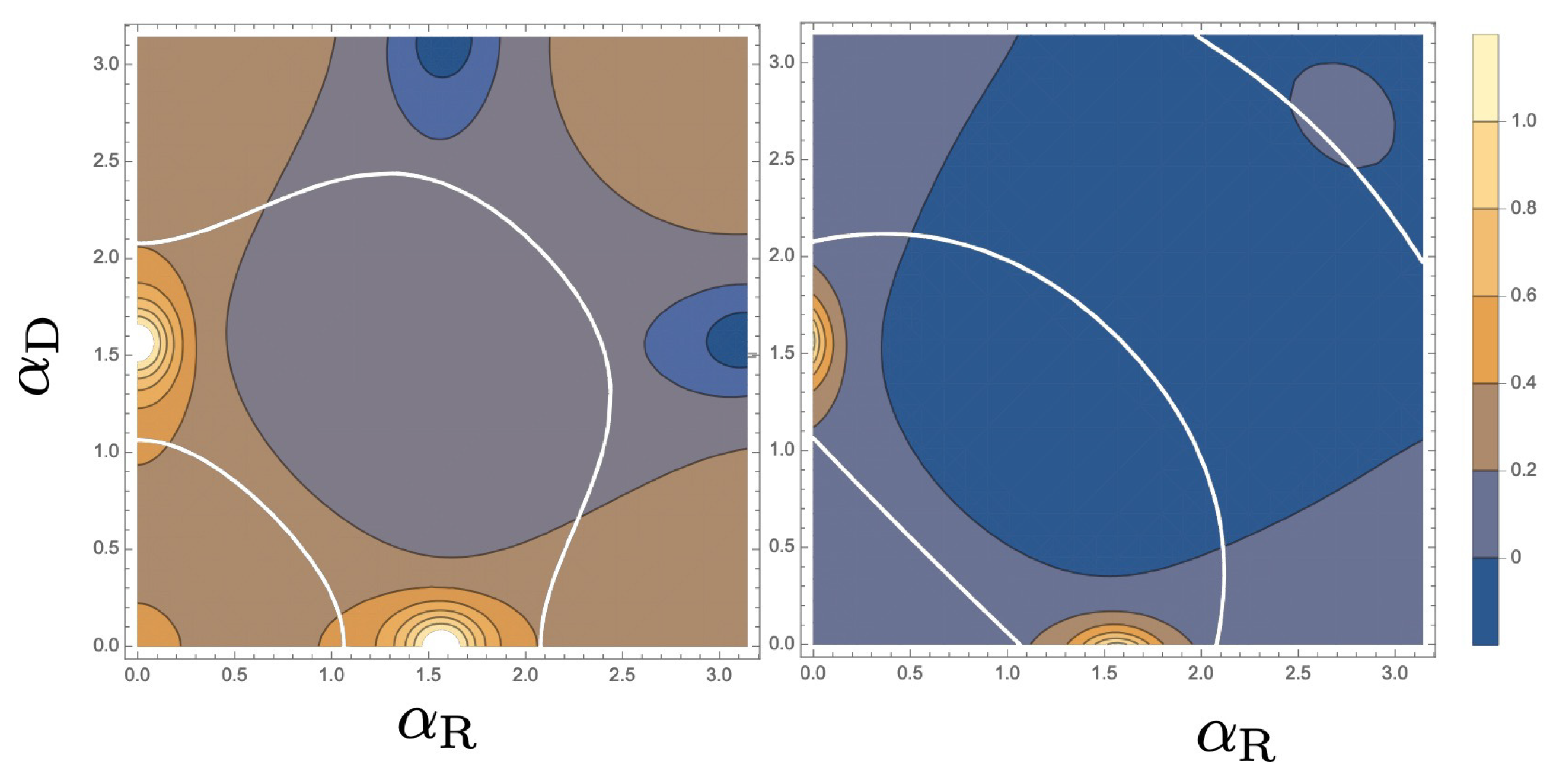
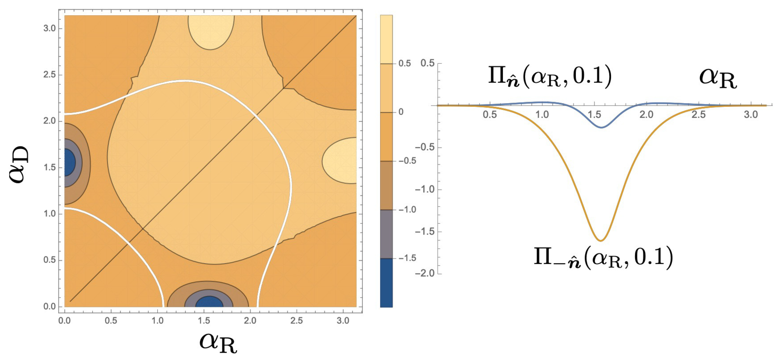
In the current analysis, the control parameters are assumed to purely modulate the phase of the electrons. In real experiments, unintended modulation of hopping amplitudes, $J_{uv}$, or the site energies, ${ϵ}_b$ or ${ϵ}_c$ by the gate voltages may induce additional effects. We demonstrated that by using the two types of the SOI as the two control parameters, spin-QAP is possible. However, in the experiments, independent control of the Rashba SOI and Dresselhaus SOI will be a complicated task. Fortunately, as shown in Figure 6, the area of large Berry curvature is well isolated and the tiny change of Dresselhaus SOI may be sufficient to observe QAP. It would be interesting if other types of SOI interaction [5] could be another control parameter of the QAP.

References

- Bercioux, D.; Lucignano, P. Quantum transport in Rashba spin-orbit materials: A review. Rep. Prog. Phys. 2015, 78, 106001. [Google Scholar] [CrossRef] [PubMed]
- Nitta, J.; Akazaki, T.; Takayanagi, H.; Enoki, T. Gate Control of Spin-Orbit Interaction in an Inverted In0.53Ga0.47As/In0.52Al0.48As Heterostructure. Phys. Rev. Lett 1997, 78, 1335. [Google Scholar] [CrossRef]
- Aharony, A.; Tokura, Y.; Cohen, G.Z.; Entin-Wohlman, O.; Katsumoto, S. Filtering and analyzing mobile qubit information via Rashba-Dresselhaus-Aharonov-Bohm interferometers. Phys. Rev. B 2011, 84, 035323. [Google Scholar] [CrossRef]
- Matityahu, S.; Aharony, A.; Entin-Wohlman, O.; Tarucha, S. Spin filtering in a Rashba-Dresselhaus-Aharonov-Bohm double-dot interferometer. New J. Phys. 2013, 15, 125017. [Google Scholar] [CrossRef]
- Kondo, K. Spin filter effects in an Aharonov-Bohm ring with double quantum dots under general Rashba spin-orbit interactions. New J. Phys. 2016, 18, 013002. [Google Scholar] [CrossRef]
- Tu, M.W.-Y.; Aharony, A.; Zhang, W.-M.; Entin-Wohlman, O. Real-time dynamics of spin-dependent transport through a double-quantum-dot Aharonov-Bohm interferometer with spin-orbit interaction. Phys. Rev. B 2014, 90, 165422. [Google Scholar] [CrossRef]
- Watson, S.K.; Potok, R.M.; Marcus, C.M.; Umansky, V. Experimental Realization of a Quantum Spin Pump. Phys. Rev. Lett. 2003, 91, 258301. [Google Scholar] [CrossRef]
- Sharma, P.; Brouwer, P.W. Mesoscopic Effects in Adiabatic Spin Pumping. Phys. Rev. Lett. 2003, 91, 166801. [Google Scholar] [CrossRef]
- Averin, D.V.; Möttönen, M.; Pekola, J.P. Maxwell’s demon based on a single-electron pump. Phys. Rev. B 2011, 84, 245448. [Google Scholar] [CrossRef]
- Zhang, P.; Xue, Q.-K.; Xie, X.C. Spin Current through a Quantum Dot in the Presence of an Oscillating Magnetic Field. Phys. Rev. Lett. 2003, 91, 196602. [Google Scholar] [CrossRef]
- Aono, T. Adiabatic spin pumping through a quantum dot with a single orbital level. Phys. Rev. B 2003, 67, 155303. [Google Scholar] [CrossRef]
- Nakajima, S.; Taguchi, M.; Kubo, T.; Tokura, Y. Interaction effect on adiabatic pump of charge and spin in quantum dot. Phys. Rev. B 2015, 92, 195420. [Google Scholar] [CrossRef]
- Hashimoto, K.; Tatara, G.; Uchiyama, C. Nonadiabaticity in spin pumping under relaxation. Phys. Rev. B 2017, 96, 064439. [Google Scholar] [CrossRef]
- Tserkovnyak, Y.; Brataas, A.; Bauer, G.E.W. Spin pumping and magnetization dynamics in metallic multilayers. Phys. Rev. B 2002, 66, 224403. [Google Scholar] [CrossRef]
- Winkler, N.; Governale, M.; König, J. Theory of spin pumping through an interacting quantum dot tunnel coupled to a ferromagnet with time-dependent magnetization. Phys. Rev. B 2013, 87, 155428. [Google Scholar] [CrossRef]
- Chen, K.; Zhang, S. Spin Pumping in the Presence of Spin-Orbit Coupling. Phys. Rev. Lett. 2015, 114, 126602. [Google Scholar] [CrossRef]
- Tatara, G.; Mizukami, S. Consistent microscopic analysis of spin pumping effects. Phys. Rev. B 2017, 96, 064423. [Google Scholar] [CrossRef]
- Büttiker, M.; Thomas, H.; Prêtre, A. Current partition in multiprobe conductors in the presence of slowly oscillating external potentials. Z. Phys. B 1994, 94, 133. [Google Scholar] [CrossRef]
- Brouwer, P.W. Scattering approach to parametric pumping. Phys. Rev. B 1998, 58, R10135. [Google Scholar] [CrossRef]
- Levinson, Y.; Entin-Wohlman, O.; Wölfle, P. Pumping at resonant transmission and transferred charge quantization. Phys. A 2001, 302, 335. [Google Scholar] [CrossRef]
- Hiltscher, B.; Governale, M.; König, J. Interference and interaction effects in adiabatic pumping through quantum dots. Phys. Rev. B 2010, 81, 085302. [Google Scholar] [CrossRef]
- Sau, J.D.; Kitagawa, T.; Halperin, B. Conductance beyond the Landauer limit and charge pumping in quantum wires. Phys. Rev. B 2012, 85, 155425. [Google Scholar] [CrossRef]
- Calvo, H.L.; Classen, L.; Splettstoesser, J.; Wegewijs, M.R. Interaction-induced charge and spin pumping through a quantum dot at finite bias. Phys. Rev. B 2012, 86, 245308. [Google Scholar] [CrossRef]
- Pluecker, T.; Wegewijs, M.R.; Splettstoesser, J. Gauge freedom in observables and Landsberg’s nonadiabatic geometric phase: Pumping spectroscopy of interacting open quantum systems. Phys. Rev. B 2017, 95, 155431. [Google Scholar] [CrossRef]
- Nakajima, S.; Tokura, Y. Excess Entropy Production in Quantum System: Quantum Master Equation Approach. J. Stat. Phys. 2017, 169, 902. [Google Scholar] [CrossRef]
- Taguchi, M.; Nakajima, S.; Kubo, T.; Tokura, Y. Quantum Adiabatic Pumping by Modulating Tunnel Phase in Quantum Dots. J. Phys. Soc. Jpn. 2016, 85, 084704. [Google Scholar] [CrossRef]
- Oreg, Y.; Entin-Wohlman, O. Transmissions through low-dimensional mesoscopic systems subject to spin-orbit scattering. Phys. Rev. B 1992, 46, 2393. [Google Scholar] [CrossRef]
© 2019 by the author. Licensee MDPI, Basel, Switzerland. This article is an open access article distributed under the terms and conditions of the Creative Commons Attribution (CC BY) license (http://creativecommons.org/licenses/by/4.0/).