Comparing Information Metrics for a Coupled Ornstein–Uhlenbeck Process


Abstract
1. Introduction
2. Information Length and Other Metrics
2.1. Information Length
2.2. Other Metrics
2.2.1. Euclidean norm
2.2.2. Wootters’ Distance
2.2.3. Kullback-Leibler Relative Entropy
2.2.4. Jensen Divergence
3. The O-U Process
3.1. Information Length
3.2. Wootters’ Distance
3.3. Kullback–Leibler Relative Entropy
3.4. Jensen Divergence
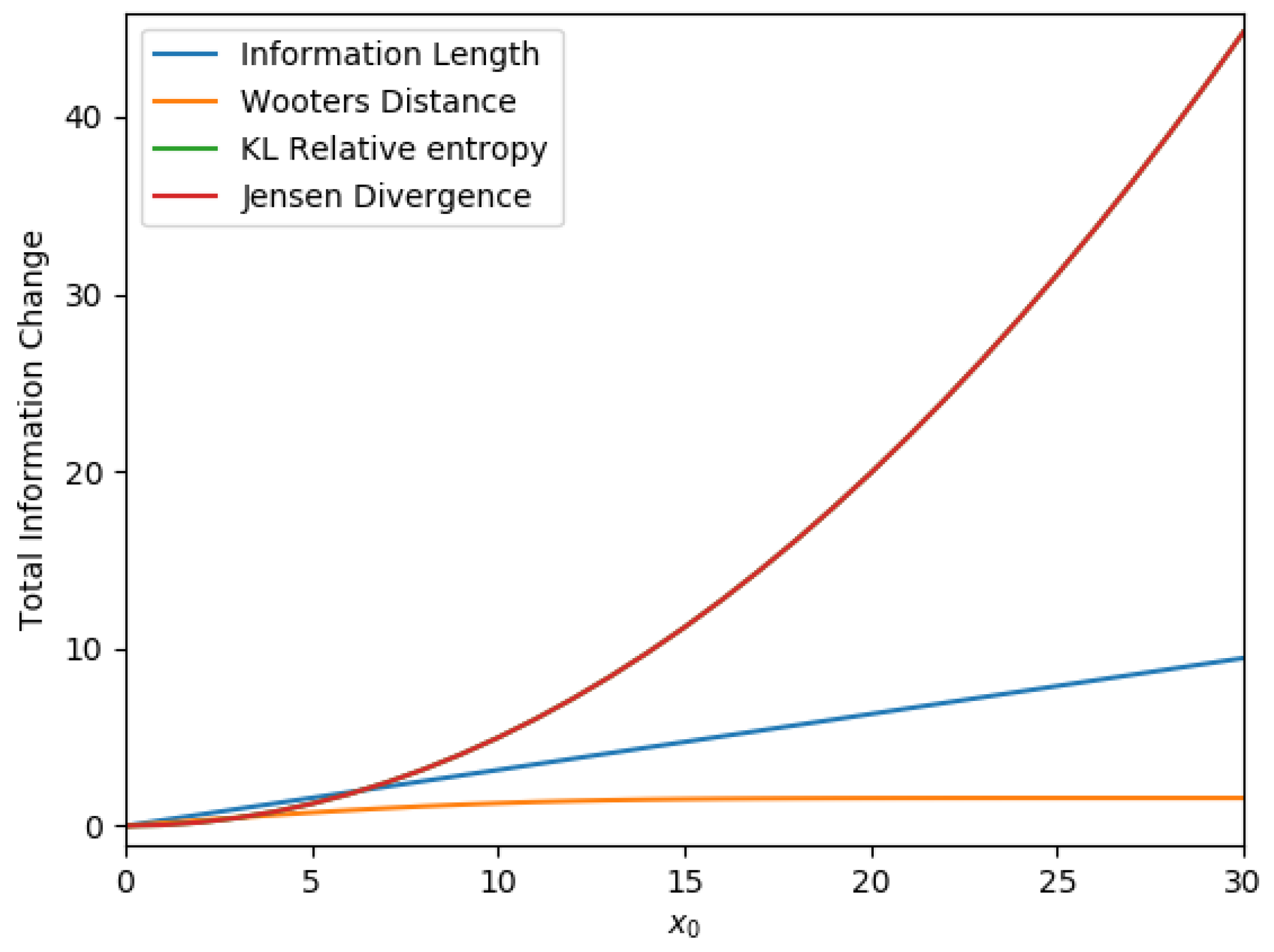
3.5. Comparison
4. The Coupled O-U Process
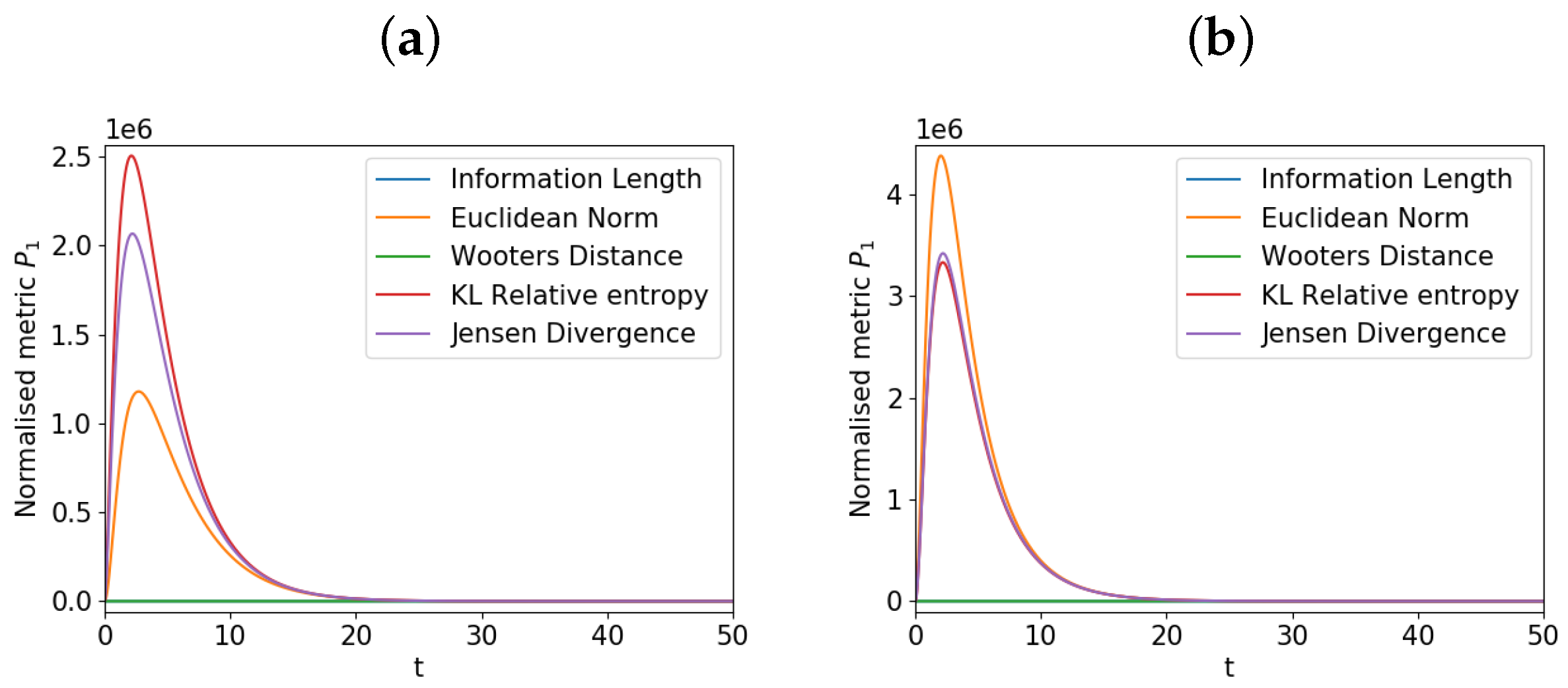
5. Results for the Coupled O-U Process
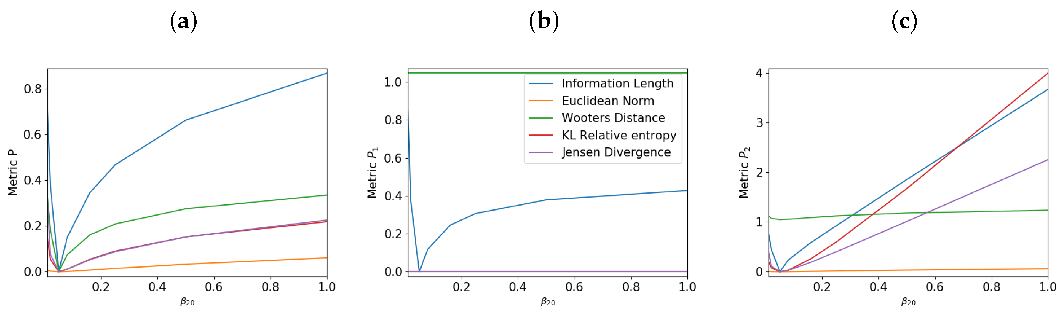
5.1. Varying
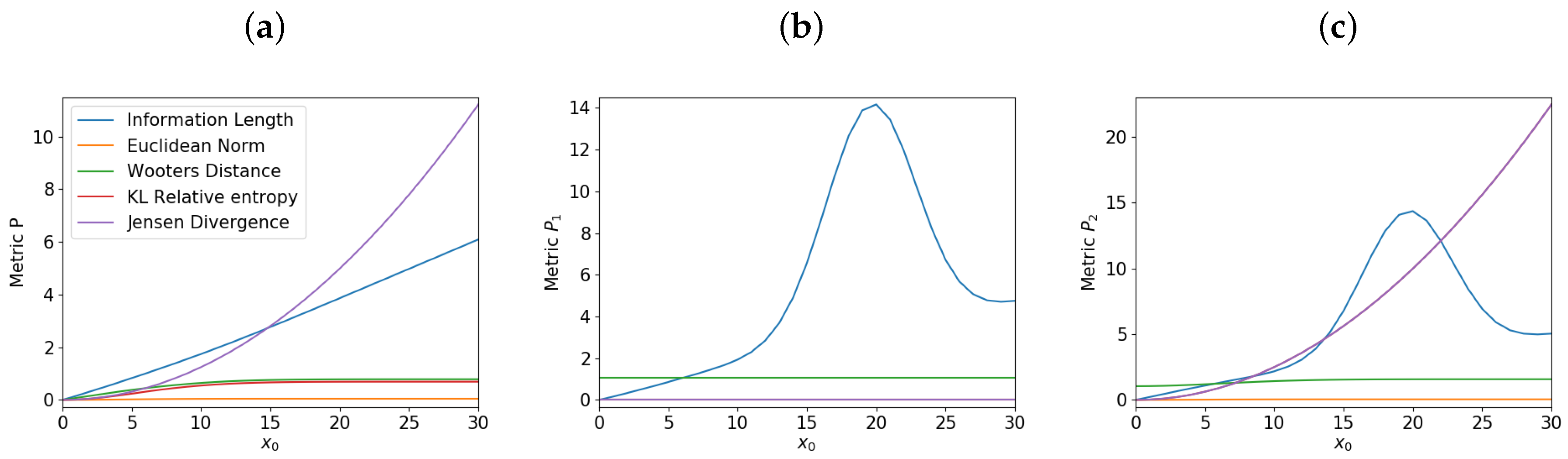
5.2. Varying
6. Conclusions
Author Contributions
Funding
Conflicts of Interest
Appendix A
Appendix A.1. The O-U Process


Appendix A.2. Coupled O-U Process
Appendix B
References
- Zamir, R. A proof of the Fisher information inequality via a data processing argument. IEEE Trans. Inf. Theory 1998, 44, 1246–1250. [Google Scholar] [CrossRef]
- Gibbs, A.L.; Su, F.E. On choosing and bounding probability metrics. Int. Stat. Rev. 2002, 70, 419–435. [Google Scholar] [CrossRef]
- Jordan, R.; Kinderlehrer, D.; Otto, F. The variational formulation of the Fokker–Planck equation. SIAM J. Math. Anal. 1998, 29, 1–17. [Google Scholar] [CrossRef]
- Lott, J. Some geometric calculations on Wasserstein space. Commun. Math. Phys. 2008, 277, 423–437. [Google Scholar] [CrossRef]
- Takatsu, A. Wasserstein geometry of Gaussian measures. Osaka J. Math. 2011, 48, 1005–1026. [Google Scholar]
- Otto, F.; Villani, C. Generalization of an Inequality by Talagrand and Links with the Logarithmic Sobolev Inequality. J. Funct. Anal. 2000, 173, 361–400. [Google Scholar] [CrossRef]
- Costa, S.; Santos, S.; Strapasson, J. Fisher information distance. Discret. Appl. Math. 2015, 197, 59–69. [Google Scholar] [CrossRef]
- Frieden, B.R. Science from Fisher Information; Cambridge University Press: Cambridge, UK, 2004. [Google Scholar]
- Wootters, W.K. Statistical distance and Hilbert space. Phys. Rev. D 1981, 23, 357–362. [Google Scholar] [CrossRef]
- Kullback, S. Letter to the Editor: The Kullback-Leibler distance. Am. Stat. 1951, 41, 340–341. [Google Scholar]
- Kowalski, A.M.; Martin, M.T.; Plastino, A.; Rosso, O.A.; Casas, M. Distances in Probability Space and the Statistical Complexity Setup. Entropy 2011, 13, 1055–1075. [Google Scholar] [CrossRef]
- Information Length. Available online: https://encyclopedia.pub/238 (accessed on 29 July 2019).
- Heseltine, J.; Kim, E. Novel mapping in non-equilibrium stochastic processes. J. Phys. A 2016, 49, 175002. [Google Scholar] [CrossRef]
- Kim, E. Investigating Information Geometry in Classical and Quantum Systems through Information Length. Entropy 2018, 20, 574. [Google Scholar] [CrossRef]
- Kim, E.; Lewis, P. Information length in quantum systems. J. Stat. Mech. 2018, 043106. [Google Scholar] [CrossRef]
- Kim, E.; Hollerbach, R. Signature of nonlinear damping in geometric structure of a nonequilibrium process. Phys. Rev. E 2017, 95, 022137. [Google Scholar] [CrossRef]
- Kim, E.; Hollerbach, R. Geometric structure and information change in phase transitions. Phys. Rev. E 2017, 95, 062107. [Google Scholar] [CrossRef]
- Hollerbach, R.; Dimanche, D.; Kim, E. Information geometry of nonlinear stochastic systems. Entropy 2018, 20, 550. [Google Scholar] [CrossRef]
- Hollerbach, R.; Kim, E.; Mahi, Y. Information length as a new diagnostic in the periodically modulated double-well model of stochastic resonance. Physica A 2019, 525, 1313–1322. [Google Scholar] [CrossRef]
- Kim, E.; Hollerbach, R. Time-dependent probability density function in cubic stochastic processes. Phys. Rev. E 2016, 94, 052118. [Google Scholar] [CrossRef]
- Nicholson, S.B.; Kim, E. Investigation of the statistical distance to reach stationary distributions. Phys. Lett. A 2015, 379, 83–88. [Google Scholar] [CrossRef]
- Matey, A.; Lamberti, P.W.; Martin, M.T.; Plastron, A. Wotters’ distance resisted: A new distinguishability criterium. Eur. Rhys. J. D 2005, 32, 413–419. [Google Scholar]
- Risken, H. The Fokker-Planck Equation: Methods of Solution and Applications; Springer: Berlin, Germany, 1996. [Google Scholar]
- Klebaner, F. Introduction to Stochastic Calculus with Applications; Imperial College Press: London, UK, 2012. [Google Scholar]
- Bena, I. Dichotomous Markov Noise: Exact results for out-of-equilibrium systems (a brief overview). Int. J. Mod. Phys. B 2006, 20, 2825–2888. [Google Scholar] [CrossRef]
- Shwartz-Ziv, R.; Tishby, N. Opening the Black Box of Deep Neural Networks via Information. arXiv 2017, arXiv:1703.00810. [Google Scholar]
- Kim, E.; Lee, U.; Heseltine, J.; Hollerbach, R. Geometric structure and geodesic in a solvable model of nonequilibrium process. Phys. Rev. E 2016, 93, 062127. [Google Scholar] [CrossRef]
- Van Den Brock, C. On the relation between white shot noise, Gaussian white noise, and the dichotomic Markov process. J. Stat. Phys. 1983, 31, 467–483. [Google Scholar] [CrossRef]


© 2019 by the authors. Licensee MDPI, Basel, Switzerland. This article is an open access article distributed under the terms and conditions of the Creative Commons Attribution (CC BY) license (http://creativecommons.org/licenses/by/4.0/).
Share and Cite
Heseltine, J.; Kim, E.-j. Comparing Information Metrics for a Coupled Ornstein–Uhlenbeck Process. Entropy 2019, 21, 775. https://doi.org/10.3390/e21080775
Heseltine J, Kim E-j. Comparing Information Metrics for a Coupled Ornstein–Uhlenbeck Process. Entropy. 2019; 21(8):775. https://doi.org/10.3390/e21080775
Chicago/Turabian StyleHeseltine, James, and Eun-jin Kim. 2019. "Comparing Information Metrics for a Coupled Ornstein–Uhlenbeck Process" Entropy 21, no. 8: 775. https://doi.org/10.3390/e21080775
APA StyleHeseltine, J., & Kim, E.-j. (2019). Comparing Information Metrics for a Coupled Ornstein–Uhlenbeck Process. Entropy, 21(8), 775. https://doi.org/10.3390/e21080775