A Novel Method for Intelligent Single Fault Detection of Bearings Using SAE and Improved D–S Evidence Theory


Abstract
:1. Introduction
- (1)
- The problem about how to realize intelligent single fault detection (SFD) from multi-fault by the features auto-extraction method was presented in this paper. This paper considered training the classifiers to distinguish whether data contains the single target fault or not, and the completed classifier can be the identification tool of the specific fault type trained before.
- (2)
- This paper proposed one feature auto-extraction method of SAE to process vibration data of different sensors. For the multi-sensor and multi-species faults coupling data features extraction, SAE demonstrates excellent computing and feature compression capabilities, extracted features are important for the single fault detection in this study.
- (3)
- The improved D–S evidence method for bearing fault diagnosis has been used to calculate multiple sensors’ classification results. Considering the difficulties of this data-driven method to separate faults, improving fault detection accuracy and solving the common paradoxes on traditional D–S evidence, IDS had been proposed and applied to fuse the detection results of multiple sensors.
2. Related Theory
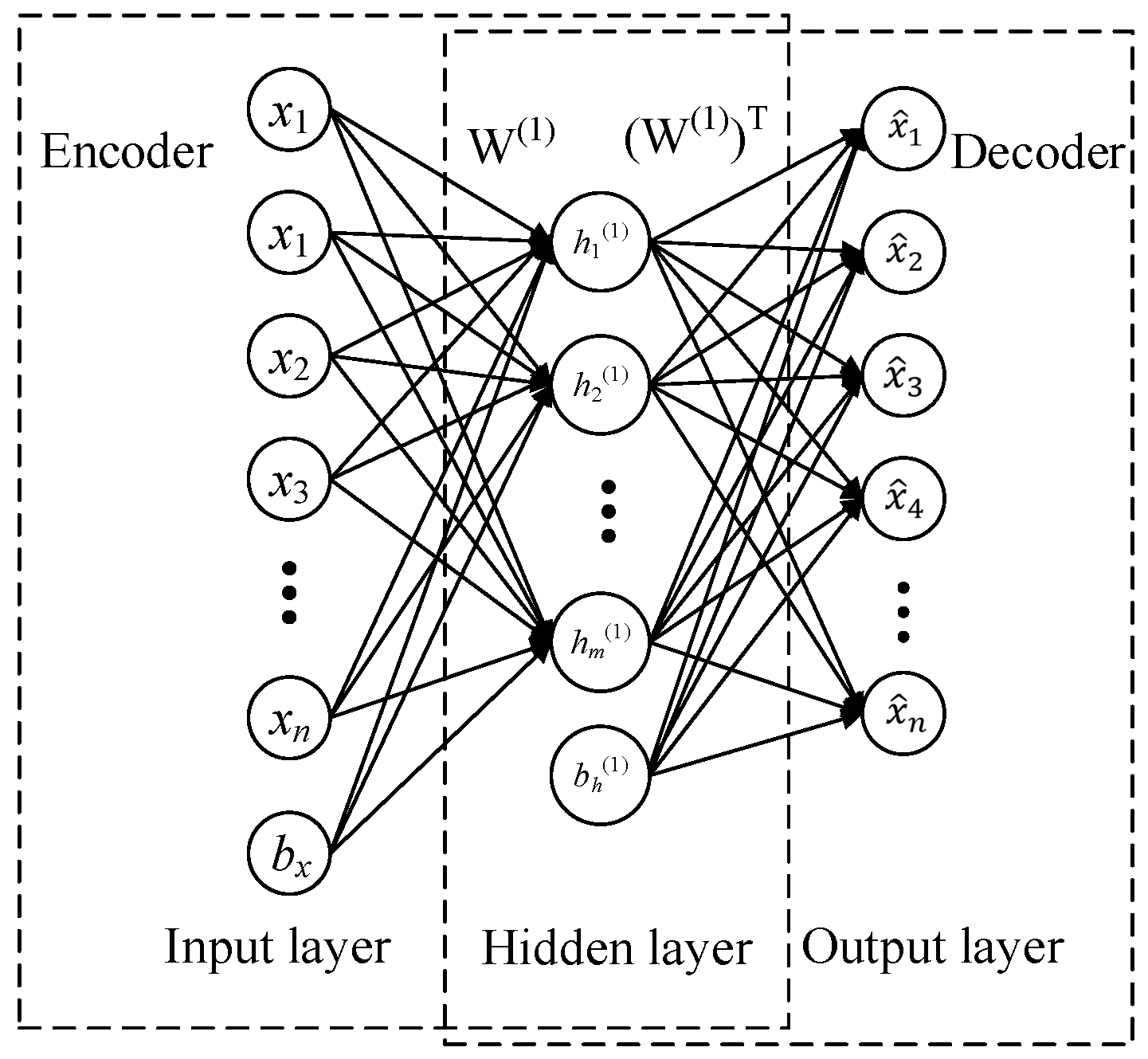
2.1. Sparse Auto-Encoder (SAE)
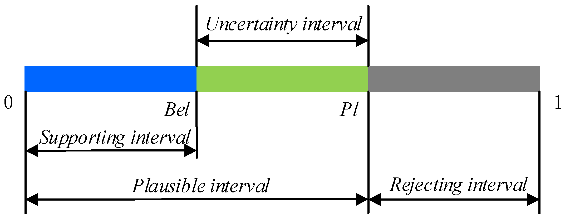
2.2. Basic Concept of D–S Evidence Theory
2.3. Pearson Correlation Coefficient (PCC)
3. The SAE and Improved D–S Evidence Theory for Bearing Single Fault Detection (SFD)
3.1. The Frame of Bearing Single Fault Detection
3.2. Rule of Single Fault Detection(R-SFD)
- (1)
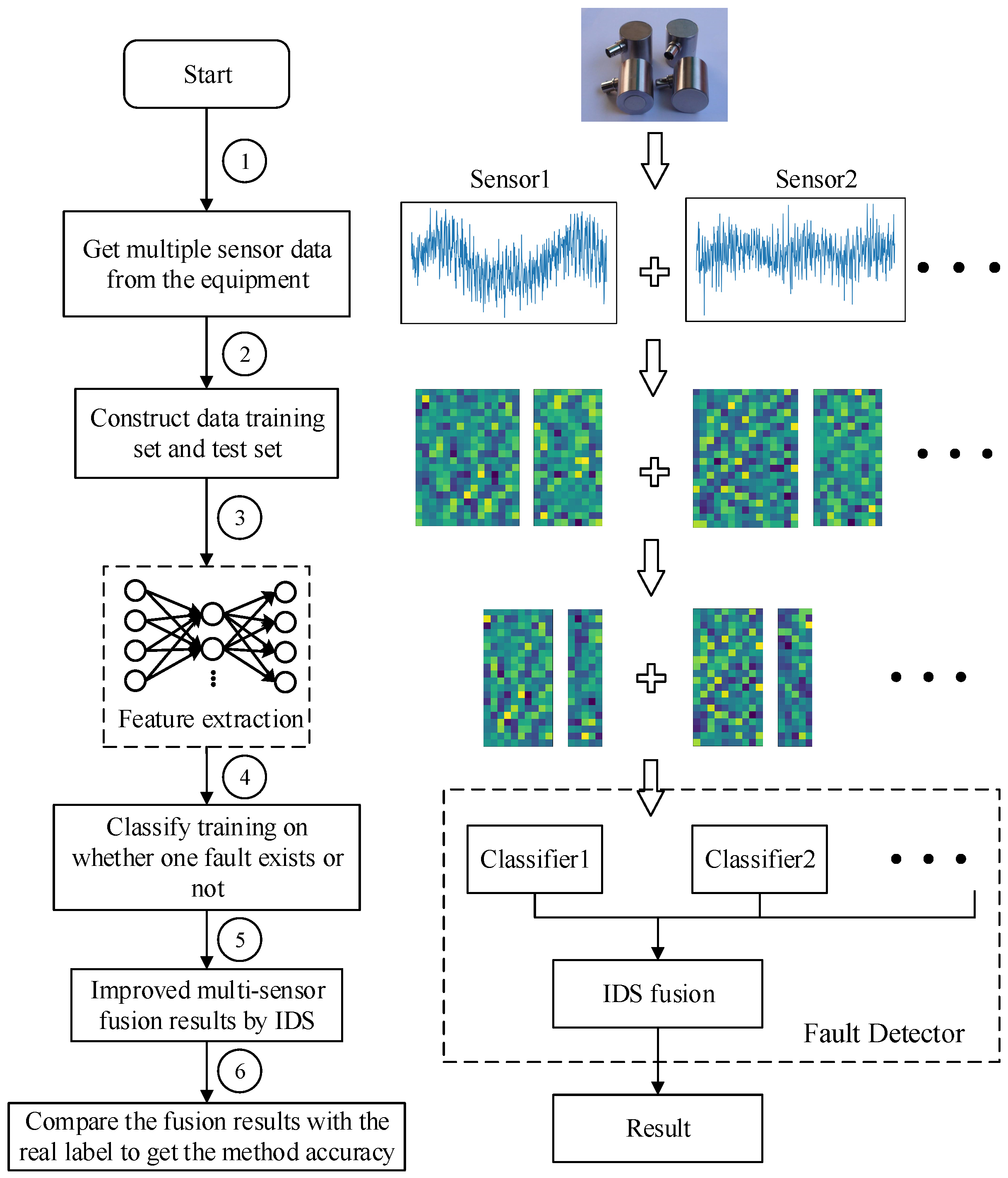
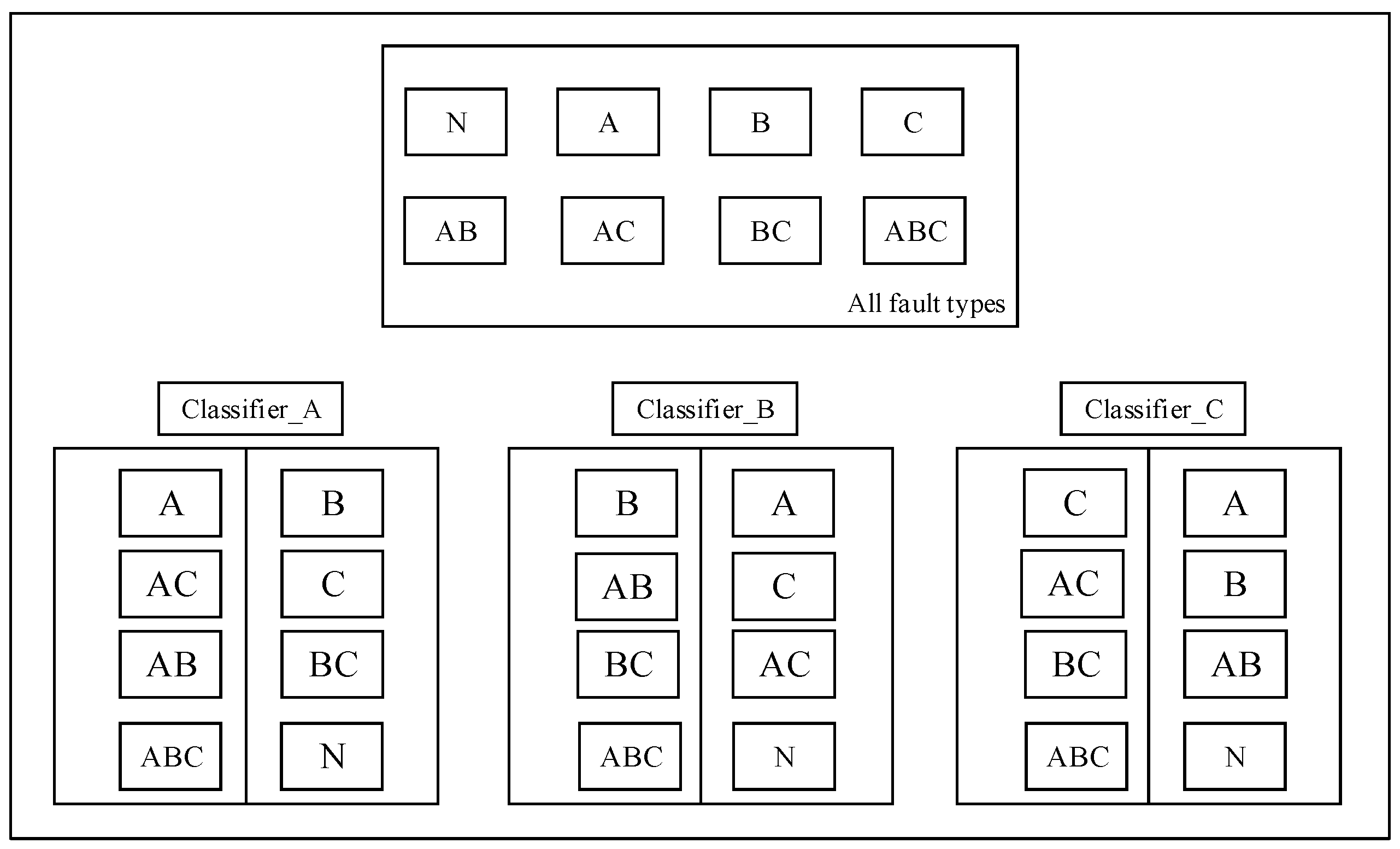
- SAE training on the sets of training samples and features extraction for each type of training data sample to obtain , and then construct , feature set , is a set of all data including a fault, for example, a single fault condition is a, b and c, combined multi-fault types are ab, ac, bc and abc, then represents a trained features set of a, ab, ac and abc. The same is true for other situations, this training principle is shown in Figure 5.
- (2)
- Here, two-category classification training is performed on the extracted features containing a certain fault and the extracted features not including the fault. For example, if the multi-fault type contains three fault conditions and the classification algorithm selects SVM, then three SVMs need to be prepared. There are two categories of training for three types of faults. The classification training results will cause the corresponding classification algorithm SVM to have the judgment ability of whether the fault exists.
- (3)
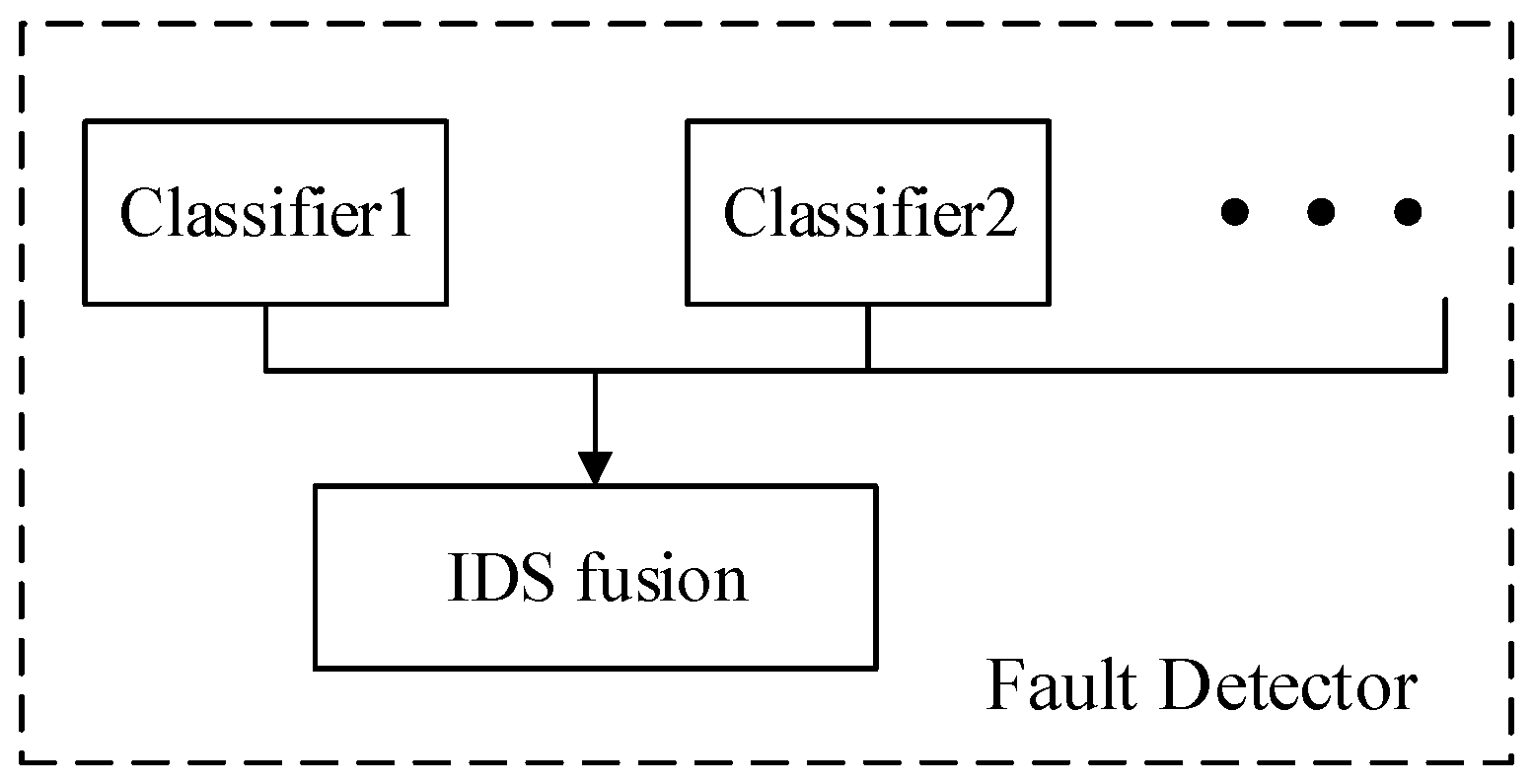
- The classified output of the plurality of sensor data was fused, and the fusion result was used for label determination. Finally, all the trained classifiers are used to test whether the faults exist in the test data, and the accuracy of the proposed method fault diagnosis is obtained. As shown in Figure 3, the test label is compared with the real label to obtain the accuracy of the proposed method in single fault detection.
3.3. The Improved D–S Evidence Theory (IDS)
- Evidence 1:
- Evidence 2:
- Evidence 3:
| Algorithm 1. “One-vote veto” eliminate |
| Input: M = , where n is the number of evidences, and X is the identification framework. Output: the modified BPA matrix. |
| for each i in for each j in X |
| if, modified it to 0.01 and make the reduce 0.01, and the always unchanged. |
| end for |
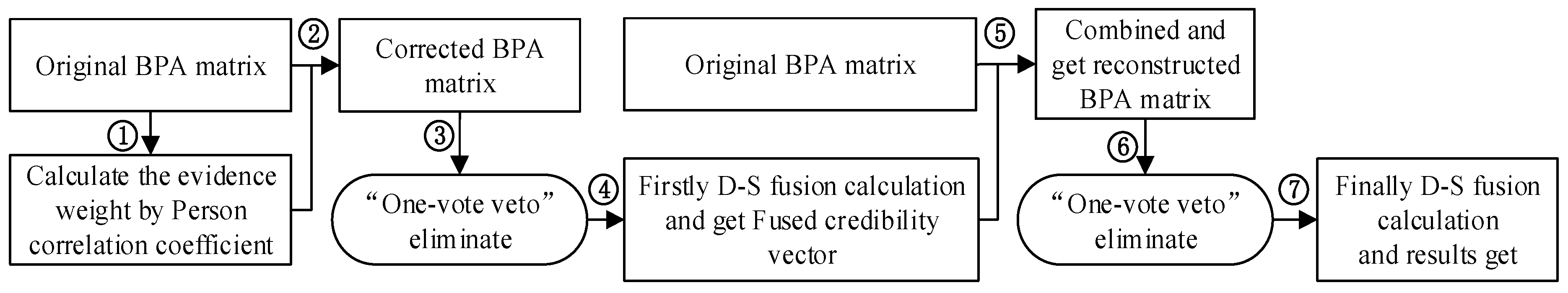
- ①
- Calculate the evidence weight by PCC, define it to , indicating the degree of correlation between and , and form a positive specific matrix based on the obtained PCC:Defining the support level of evidence as , the sum of all elements except the self in the similarity measure matrix represents the degree of support between the evidence and other evidence:Then, defining the trust degree of the evidence as , standardizing the support degree, satisfying the requirement of D–S evidence theory, , and .Finally, the evidence credibility with total negative linear correlation was set to absolute value, others remains unchanged.
- ②
- Correct the original BPA using the obtained evidence credibility . Define the corrected BPA as .
- ③
- As Algorithm 1 shows, replace 0 items to 0.01 from the corrected BPA matrix.
- ④
- According to the D–S fusion calculate rules, the first fusion support vector can be obtained.
- ⑤
- Add the BPA vector obtained from the first fusion above to original BPA matrix and get the .
- ⑥
- Modifying the 0 value of as ③ do.
- ⑦
- Perform the D–S fusion calculation once again as ④ does, and get the finally fusion results.
4. Data Acquisition and Experimental Analysis
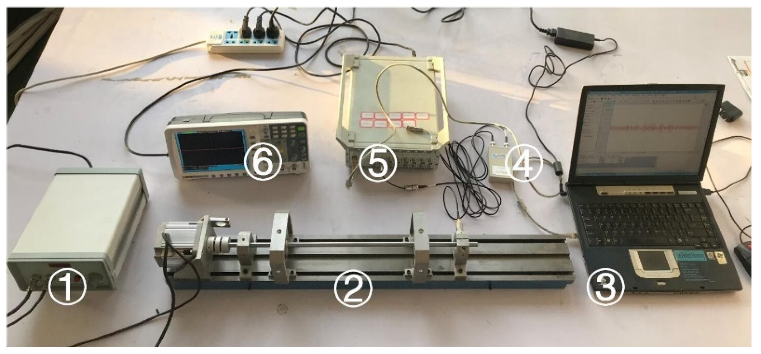
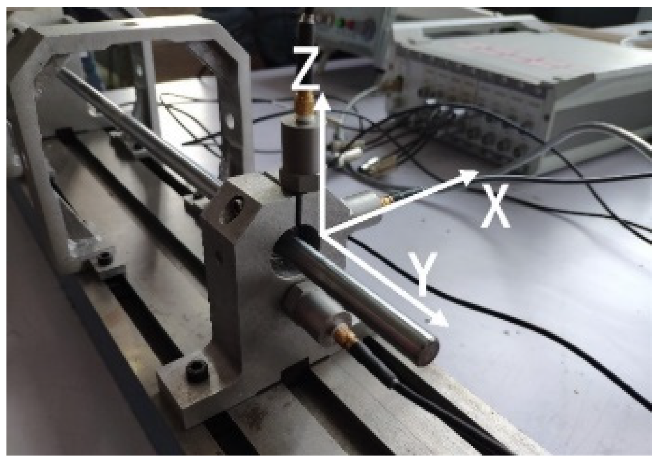
4.1. Data Preparation
4.2. Analysis
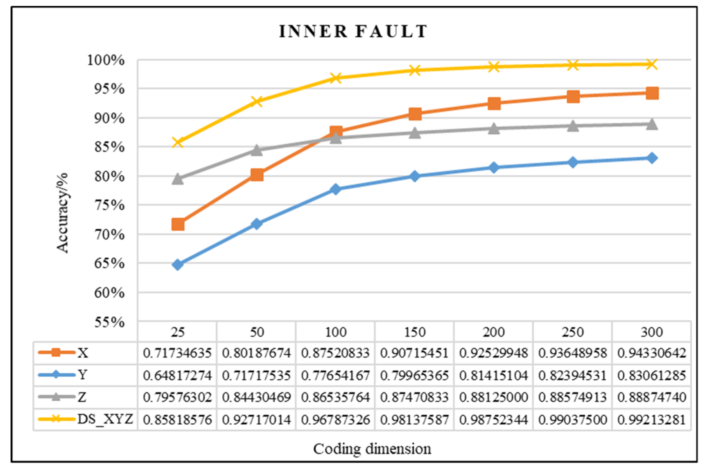
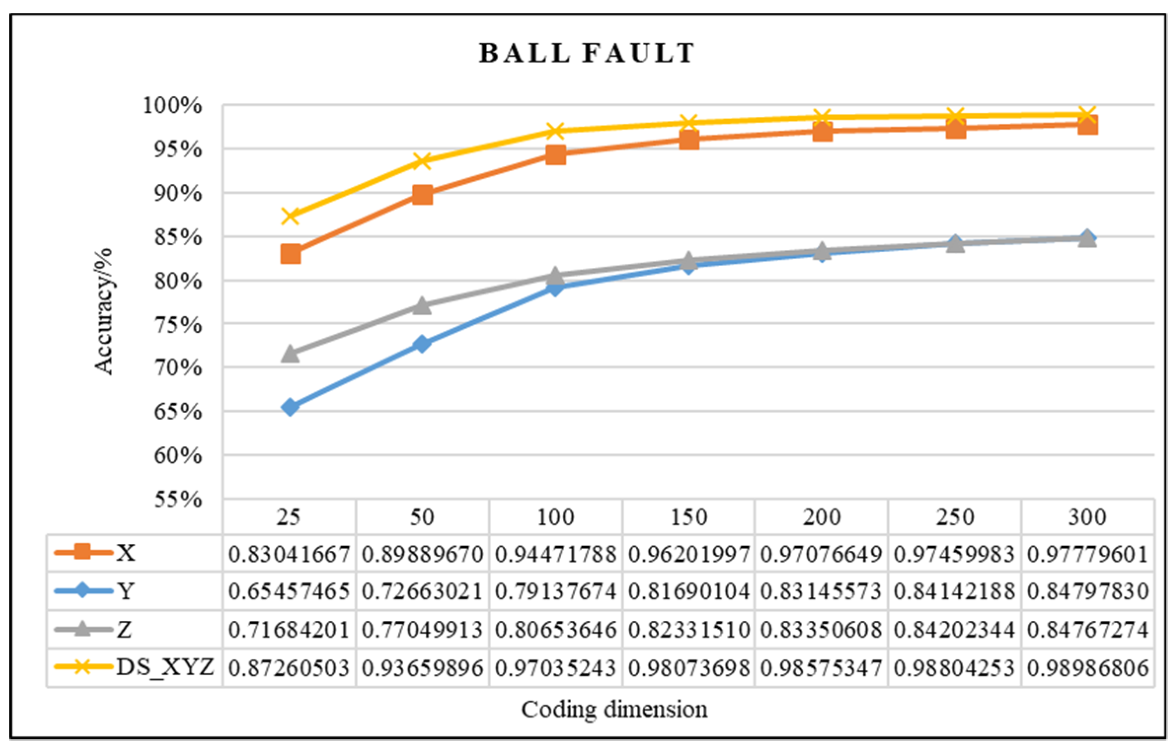
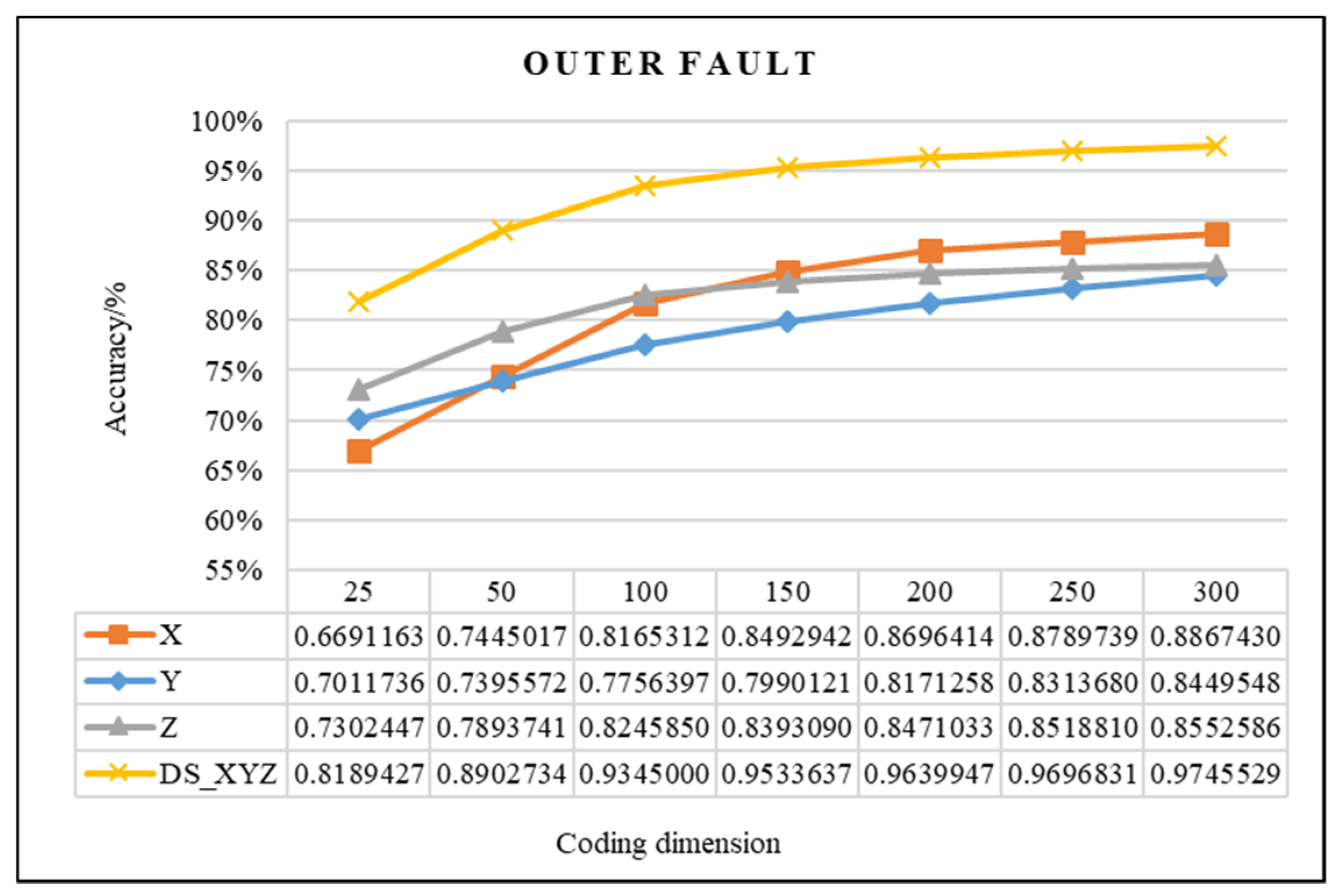
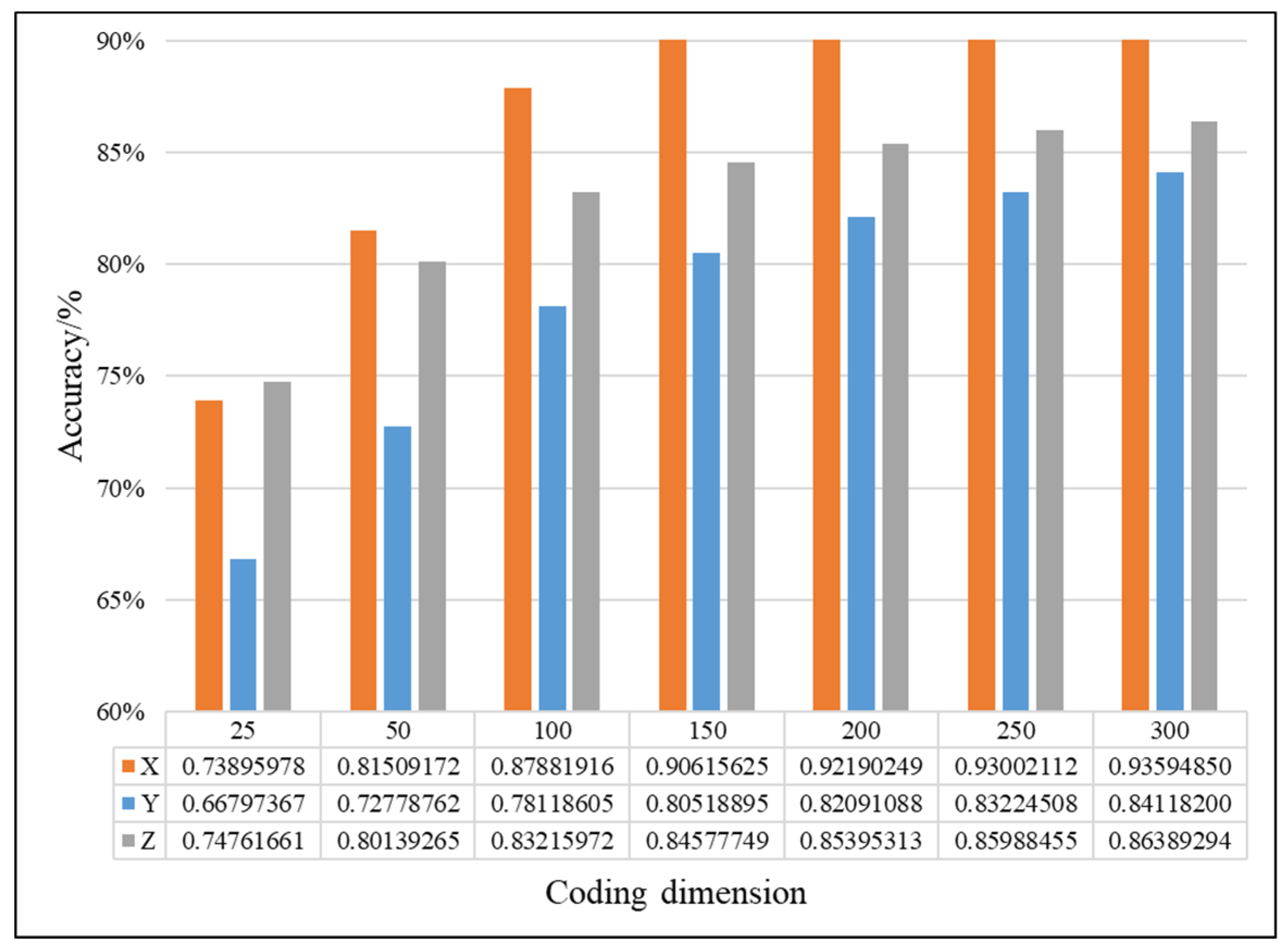
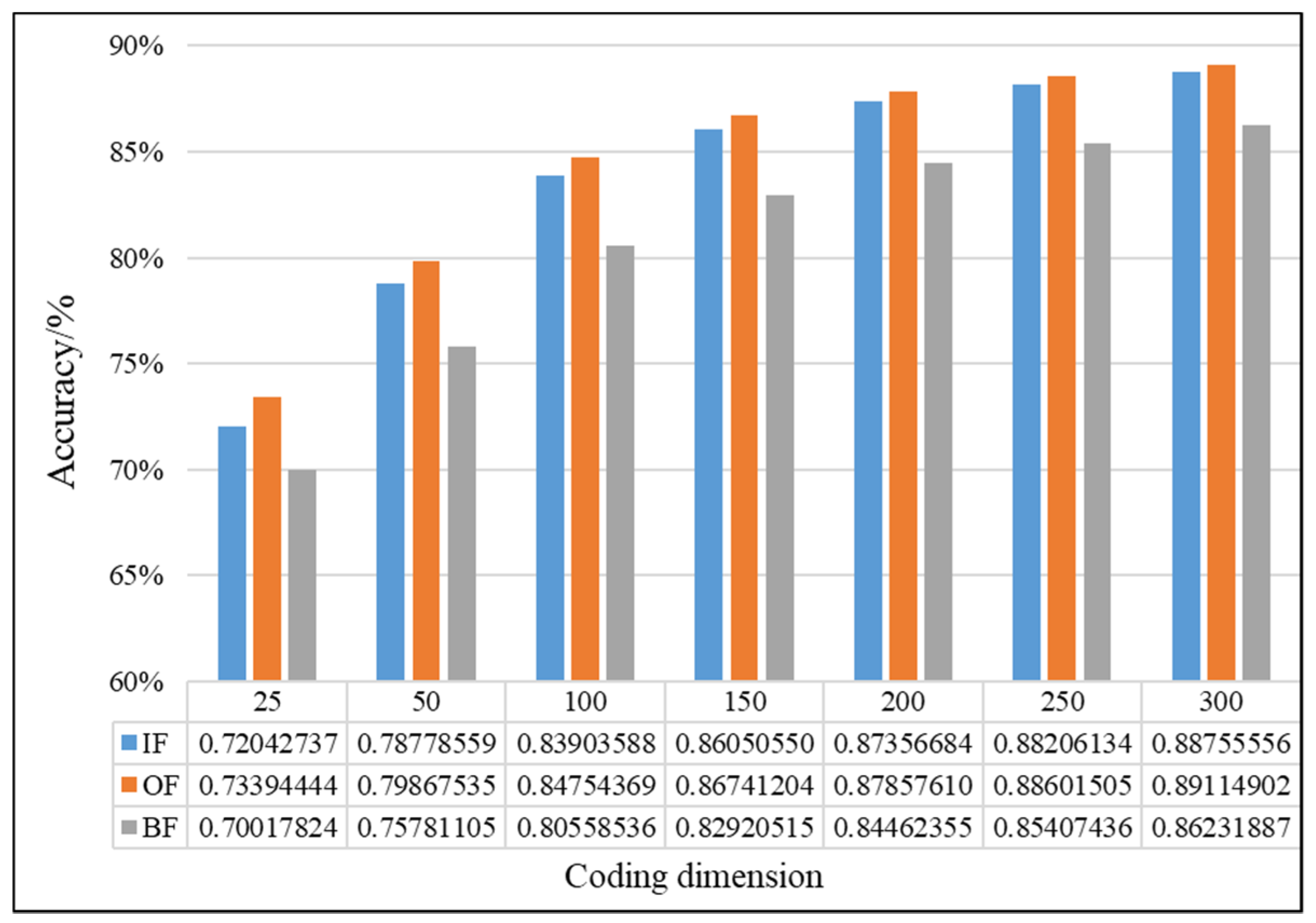
4.2.1. Effectiveness Analysis of Single Fault Detection Method by SAE and D–S Evidence Theory
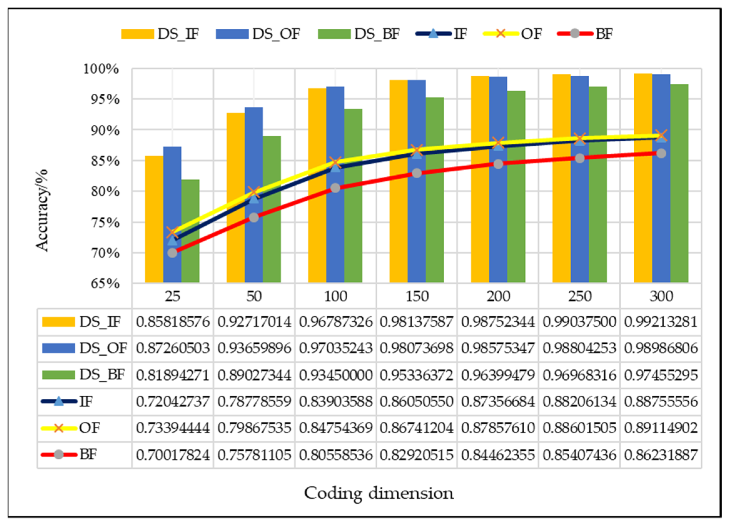
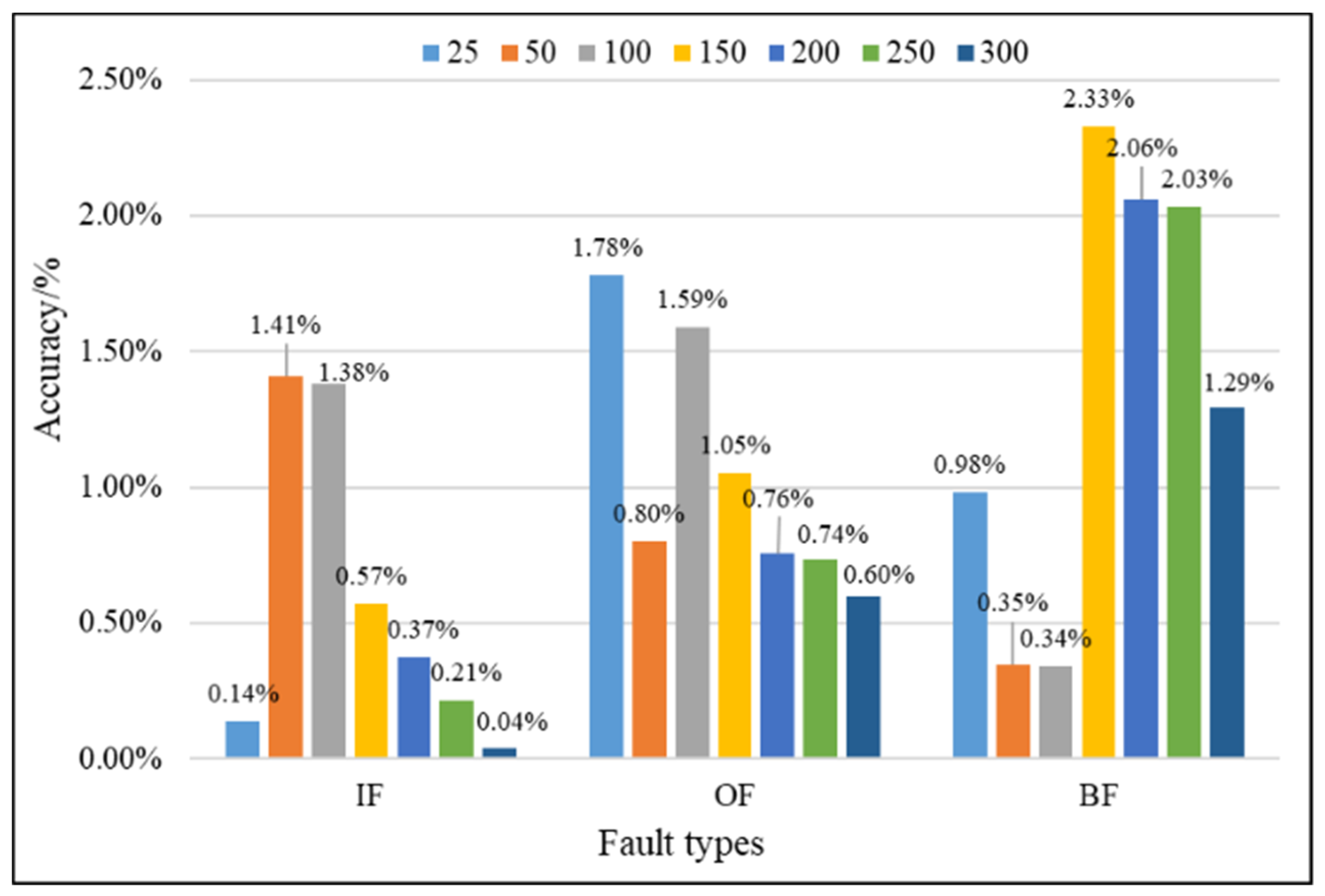
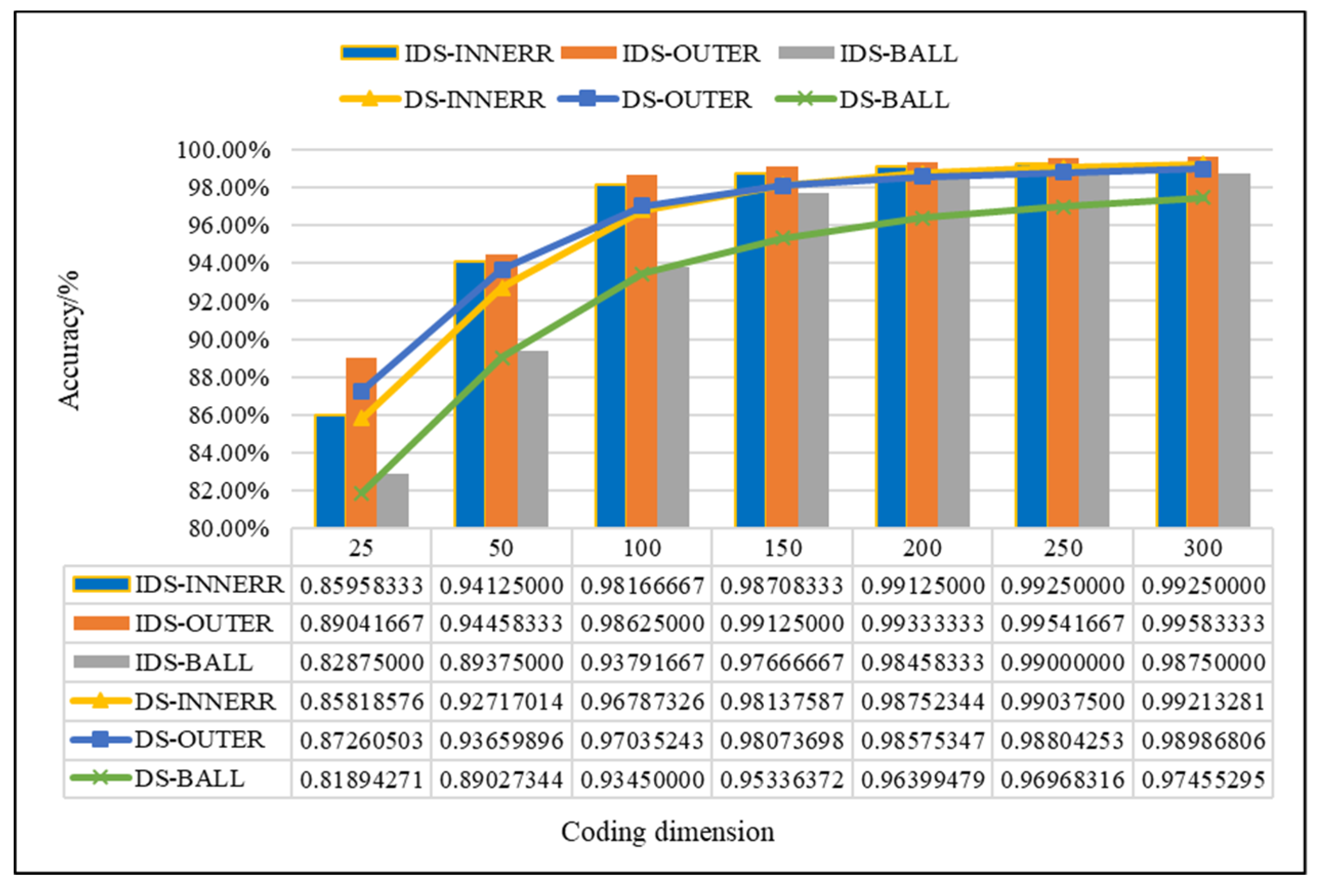
4.2.2. Evaluation of the Improved D–S (IDS) Evidence Fusion Algorithm and Its Effect in Bearing Fault Detection
5. Conclusions
Author Contributions
Funding
Conflicts of Interest
References
- Glowacz, A.; Glowacz, W.; Glowacz, Z. Early fault diagnosis of bearing and stator faults of the single-phase induction motor using acoustic signals. Measurement 2018, 113, 1–9. [Google Scholar] [CrossRef]
- Wang, L.; Liu, Z.; Miao, Q. Time–frequency analysis based on ensemble local mean decomposition and fast kurtogram for rotating machinery fault diagnosis. Mech. Syst. Signal Process. 2018, 103, 60–75. [Google Scholar] [CrossRef]
- Meng, L. An intelligent fault diagnosis system of rolling bearing. In Proceedings of the 2011 International Conference on Transportation, Mechanical, and Electrical Engineering, Changchun, China, 12–18 December 2011; pp. 544–547. [Google Scholar]
- Cerrada, M.; Sánchez, R.V.; Li, C. A review on data-driven fault severity assessment in rolling bearings. Mech. Syst. Signal Process. 2018, 99, 169–196. [Google Scholar] [CrossRef]
- Hoang, D.T.; Kang, H.J. A Bearing Fault Diagnosis Method Based on Autoencoder and Particle Swarm Optimization—Support Vector Machine. In International Conference on Intelligent Computing; Springer: Cham, Switzerland, 2018. [Google Scholar]
- Lu, C.; Wang, Z.; Zhou, B. Intelligent Fault Diagnosis of Rolling Bearing Using Hierarchical Convolutional Network Based Health State Classification; Elsevier Ltd.: New York, NY, USA, 2017; Volume 32, pp. 139–151. [Google Scholar]
- Wei, Z.; Wang, Y.; He, S. A novel intelligent method for bearing fault diagnosis based on affinity propagation clustering and adaptive feature selection. Knowl. Based Syst. 2017, 116, 1–12. [Google Scholar] [CrossRef]
- Lian, J.; Zhao, R. Fault diagnosis model based on NRS and EEMD for rolling-element bearing. In Proceedings of the Prognostics and System Health Management Conference, Harbin, China, 9–12 July 2017; pp. 1–5. [Google Scholar]
- Guo, L.; Chen, J.; Li, X. Rolling bearing fault classification based on envelope spectrum and support vector machine. J. Vib. Control 2009, 15, 1349–1363. [Google Scholar]
- Tian, Y.; Ma, J.; Lu, C. Rolling bearing fault diagnosis under variable conditions using LMD-SVD and extreme learning machine. Mech. Mach. Theory 2015, 90, 175–186. [Google Scholar] [CrossRef]
- Chen, Y.; Peng, G.; Xie, C. ACDIN: Bridging the gap between artificial and real bearing damages for bearing fault diagnosis. Neurocomputing 2018, 294, 61–71. [Google Scholar] [CrossRef]
- Zhao, D.; Li, J.; Cheng, W. Compound faults detection of rolling element bearing based on the generalized demodulation algorithm under time-varying rotational speed. J. Sound Vib. 2016, 378, 109–123. [Google Scholar] [CrossRef]
- Li, H.; Li, M.; Li, C. Multi-faults decoupling on turbo-expander using differential-based ensemble empirical mode decomposition. Mech. Syst. Signal Process. 2017, 93, 267–280. [Google Scholar] [CrossRef]
- Li, M.; Li, F.; Jing, B. Multi-fault diagnosis of rotor system based on differential-based empirical mode decomposition. J. Vib. Control 2015, 21, 1821–1837. [Google Scholar]
- Zhang, D.; Yu, D.; Zhang, W. Energy operator demodulating of optimal resonance components for the compound faults diagnosis of gearboxes. Meas. Sci. Technol. 2015, 26, 115003. [Google Scholar] [CrossRef]
- Yang, F.; Shen, X.; Wang, Z. Multi-Fault Diagnosis of Gearbox Based on Improved Multipoint Optimal Minimum Entropy Deconvolution. Entropy 2018, 20, 611. [Google Scholar] [CrossRef]
- Cui, L.; Wu, C.; Ma, C. Diagnosis of roller bearings compound fault using underdetermined blind source separation algorithm based on null-space pursuit. Shock Vib. 2015, 2015, 131489. [Google Scholar] [CrossRef]
- Purushotham, V.; Narayanan, S.; Prasad, S.A. Multi-fault diagnosis of rolling bearing elements using wavelet analysis and hidden Markov model based fault recognition. NDT E Int. 2005, 38, 654–664. [Google Scholar] [CrossRef]
- Xu, Y.; Meng, Z.; Lu, M. Compound fault diagnosis of rolling bearing based on dual-tree complex wavelet packet transform and ICA. J. Vib. Meas. Diagn. 2015, 35, 513–518. [Google Scholar]
- Chen, L.; Diao, L.; Sang, J. Weighted Evidence Combination Rule Based on Evidence Distance and Uncertainty Measure: An Application in Fault Diagnosis. Math. Probl. Eng. 2018, 2018, 5858272. [Google Scholar] [CrossRef]
- Wang, H.; Guo, L.; Dou, Z. A new method of cognitive signal recognition based on hybrid information entropy and D-S evidence theory. Mob. Netw. Appl. 2018, 23, 677–685. [Google Scholar] [CrossRef]
- Beynon, M.; Curry, B.; Morgan, P. The Dempster–Shafer theory of evidence: An alternative approach to multicriteria decision modelling. Omega 2000, 28, 37–50. [Google Scholar] [CrossRef]
- Li, H.X.; Wang, Y.; Chen, C.P. Dempster–Shafer structure based fuzzy logic system for stochastic modeling. Appl. Soft Comput. 2017, 56, 134–142. [Google Scholar] [CrossRef]
- Li, S.; Liu, G.; Tang, X. An ensemble deep convolutional neural network model with improved D-S evidence fusion for bearing fault diagnosis. Sensors 2017, 17, 1729. [Google Scholar] [CrossRef]
- Zhang, L.; Ding, L.; Wu, X. An improved Dempster–Shafer approach to construction safety risk perception. Knowl. Based Syst. 2017, 132, 30–46. [Google Scholar] [CrossRef]
- Shafer, G. A Mathematical Theory of Evidence; Princeton University Press: Princeton, NJ, USA, 1976. [Google Scholar]
- Bao, Y.; Li, H.; An, Y. Dempster–Shafer evidence theory approach to structural damage detection. Struct. Health Monit. 2012, 11, 13–26. [Google Scholar] [CrossRef]
- Li, Y.; Chen, J.; Ye, F. The improvement of D-S evidence theory and its application in IR/MMW target recognition. J. Sens. 2016, 2016, 1903792. [Google Scholar] [CrossRef]
- Yager, R.R. On the aggregation of prioritized belief structures. IEEE Trans. Syst. Man Cybern. A Syst. Hum. 1996, 26, 708–717. [Google Scholar] [CrossRef]
- Sun, Q.; Ye, X.; Gu, W. A New Combination Rules of Evidence Theory. Acta Electron. Sin. 2000, 28, 117–119. [Google Scholar]
- Murphy, C.K. Combining belief functions when evidence conflicts. Decis. Support Syst. 2000, 29, 1–9. [Google Scholar] [CrossRef]
- Deng, Y.; Shi, W.K.; Zhu, Z.F. Efficient combination approach of conflict evidence. J. Infrared Millim. Waves 2004, 23, 27–32. [Google Scholar]


| Paradoxes | Evidences | Propositions | ||||
|---|---|---|---|---|---|---|
| A | B | C | D | E | ||
| Complete conflict paradox (k = 1) | m1 | 1 | 0 | 0 | \ | \ |
| m2 | 0 | 1 | 0 | \ | \ | |
| m3 | 0.8 | 0.1 | 0.1 | \ | \ | |
| m4 | 0.8 | 0.1 | 0.1 | \ | \ | |
| 1 trust paradox (k = 0.9998) | m1 | 0.9 | 0.1 | 0 | \ | \ |
| m2 | 0 | 0.1 | 0.9 | \ | \ | |
| m3 | 0.1 | 0.15 | 0.75 | \ | \ | |
| m4 | 0.1 | 0.15 | 0.7 | \ | \ | |
| High conflict paradox (k = 0.9999) | m1 | 0.7 | 0.1 | 0.1 | 0 | 0.1 |
| m2 | 0 | 0.5 | 0.2 | 0.1 | 0.2 | |
| m3 | 0.6 | 0.1 | 0.15 | 0 | 0.15 | |
| m4 | 0.55 | 0.1 | 0.1 | 0.15 | 0.1 | |
| m5 | 0.6 | 0.1 | 0.2 | 0 | 0.1 | |
| Correlation Coefficient | Relevant Degree |
|---|---|
| 0.8–1.0 | Extremely strong |
| 0.6–0.8 | strong |
| 0.4–0.6 | Moderate |
| 0.2–0.4 | Weak |
| 0.0–0.2 | Very weak or no correlation |
| Type | Train Set Sample | Test Set Sample | Sample Length | Tags |
|---|---|---|---|---|
| N | 700 | 300 | 1024 | 000 |
| O | 700 | 300 | 1024 | 100 |
| B | 700 | 300 | 1024 | 010 |
| I | 700 | 300 | 1024 | 001 |
| OB | 700 | 300 | 1024 | 110 |
| OI | 700 | 300 | 1024 | 101 |
| BI | 700 | 300 | 1024 | 011 |
| OBI | 700 | 300 | 1024 | 111 |
| Paradoxes | Methods | Propositions | |||||
|---|---|---|---|---|---|---|---|
| A | B | C | D | E | Θ | ||
| Complete conflict paradox | Yager [29] | 0 | 0 | 0 | \ | \ | 1 |
| Sun [30] | 0.0917 | 0.0423 | 0.0071 | \ | \ | 0.8589 | |
| Murphy [31] | 0.8204 | 0.1748 | 0.0048 | \ | \ | 0 | |
| Deng [32] | 0.8166 | 0.1164 | 0.0670 | \ | \ | 0 | |
| IDS | 0.9998 | 0.0002 | 0 | \ | \ | 0 | |
| 1 trust paradox | Yager [29] | 0 | 1 | 0 | \ | \ | 0 |
| Sun [30] | 0.0388 | 0.0179 | 0.0846 | \ | \ | 0.8587 | |
| Murphy [31] | 0.1676 | 0.0346 | 0.7978 | \ | \ | 0 | |
| Deng [32] | 0.1388 | 0.1388 | 0.7294 | \ | \ | 0 | |
| IDS | 0.0003 | 0.0020 | 0.9977 | \ | \ | 0 | |
| High conflictparadox | Yager [29] | 0 | 0.3571 | 0.4286 | 0 | 0.2143 | 0 |
| Sun [30] | 0.0443 | 0.0163 | 0.0163 | 0.0045 | 0.0118 | 0.9094 | |
| Murphy [31] | 0.7637 | 0.1031 | 0.0716 | 0.0080 | 0.0538 | 0 | |
| Deng [32] | 0.5324 | 0.1521 | 0.1462 | 0.0451 | 0.1241 | 0 | |
| IDS | 0.9961 | 0.0014 | 0.0020 | 0 | 0.0005 | 0 | |
| Fault Types | Coding Dimension | Methods | ||
|---|---|---|---|---|
| D–S | IDS | Difference Value | ||
| IF | 150 | 0.98137587 | 0.98708333 | 0.57% |
| 200 | 0.98752344 | 0.99125000 | 0.37% | |
| Difference value | 0.61% | 0.42% | - | |
| OF | 150 | 0.98073698 | 0.99125000 | 1.05% |
| 200 | 0.98575347 | 0.99333333 | 0.76% | |
| Difference value | 0.50% | 0.21% | - | |
| BF | 150 | 0.95336372 | 0.97666667 | 2.33% |
| 200 | 0.96399479 | 0.98458333 | 2.06% | |
| Difference value | 1.06% | 0.79% | - | |
© 2019 by the authors. Licensee MDPI, Basel, Switzerland. This article is an open access article distributed under the terms and conditions of the Creative Commons Attribution (CC BY) license (http://creativecommons.org/licenses/by/4.0/).
Share and Cite
Lu, J.; Zhang, H.; Tang, X. A Novel Method for Intelligent Single Fault Detection of Bearings Using SAE and Improved D–S Evidence Theory. Entropy 2019, 21, 687. https://doi.org/10.3390/e21070687
Lu J, Zhang H, Tang X. A Novel Method for Intelligent Single Fault Detection of Bearings Using SAE and Improved D–S Evidence Theory. Entropy. 2019; 21(7):687. https://doi.org/10.3390/e21070687
Chicago/Turabian StyleLu, Jianguang, Huan Zhang, and Xianghong Tang. 2019. "A Novel Method for Intelligent Single Fault Detection of Bearings Using SAE and Improved D–S Evidence Theory" Entropy 21, no. 7: 687. https://doi.org/10.3390/e21070687
APA StyleLu, J., Zhang, H., & Tang, X. (2019). A Novel Method for Intelligent Single Fault Detection of Bearings Using SAE and Improved D–S Evidence Theory. Entropy, 21(7), 687. https://doi.org/10.3390/e21070687