Assessment of a Stream Gauge Network Using Upstream and Downstream Runoff Characteristics and Entropy


Abstract
:1. Introduction
2. Entropy to Assess a Stream Gauge Network
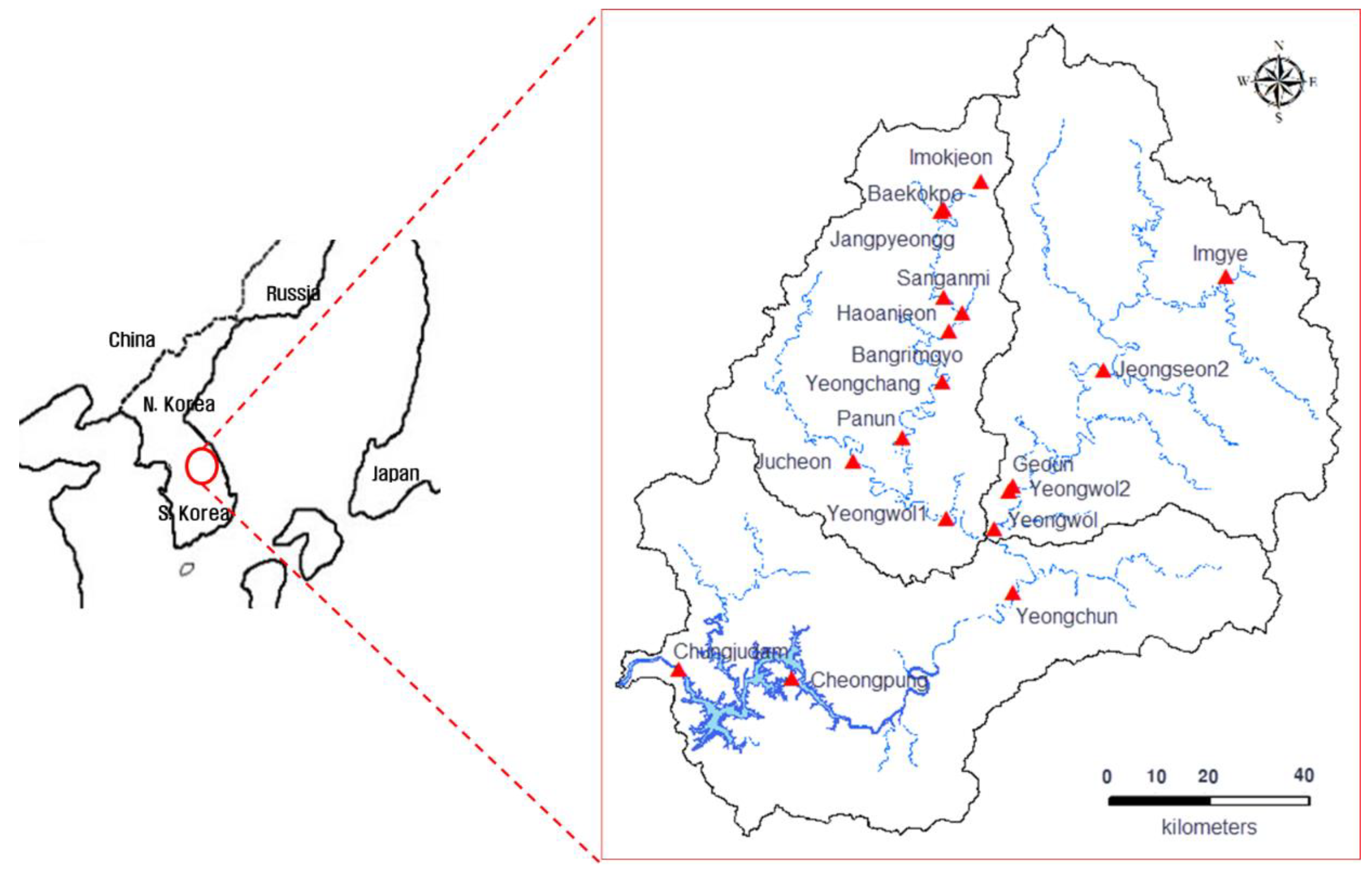
3. Study Area
3.1. Selected Study Area
3.2. Density of Stream Gauge Stations in the Study Area
4. Development of Unit Hydrographs and their Conversion to the Probability Density Function
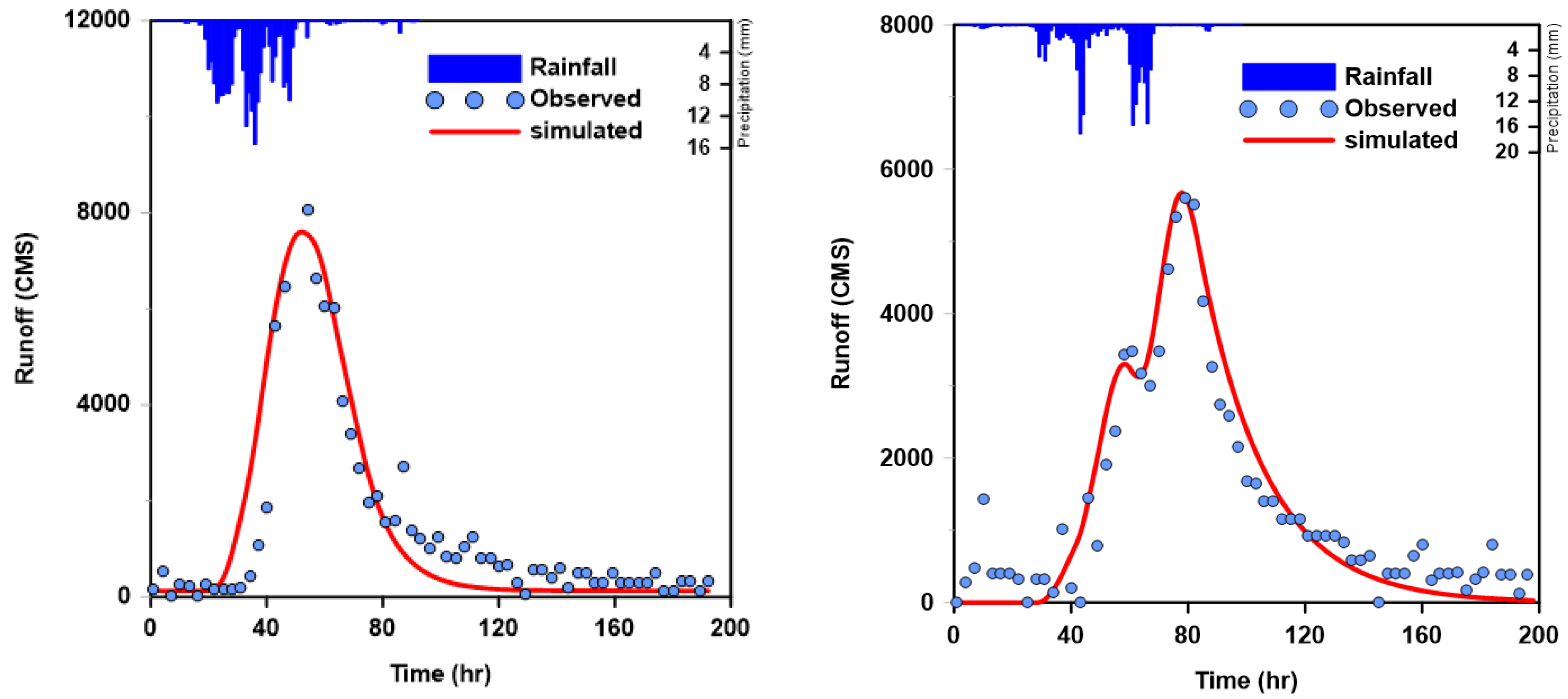
4.1. Rainfall–Runoff Analysis for the Development of Unit Hydrographs
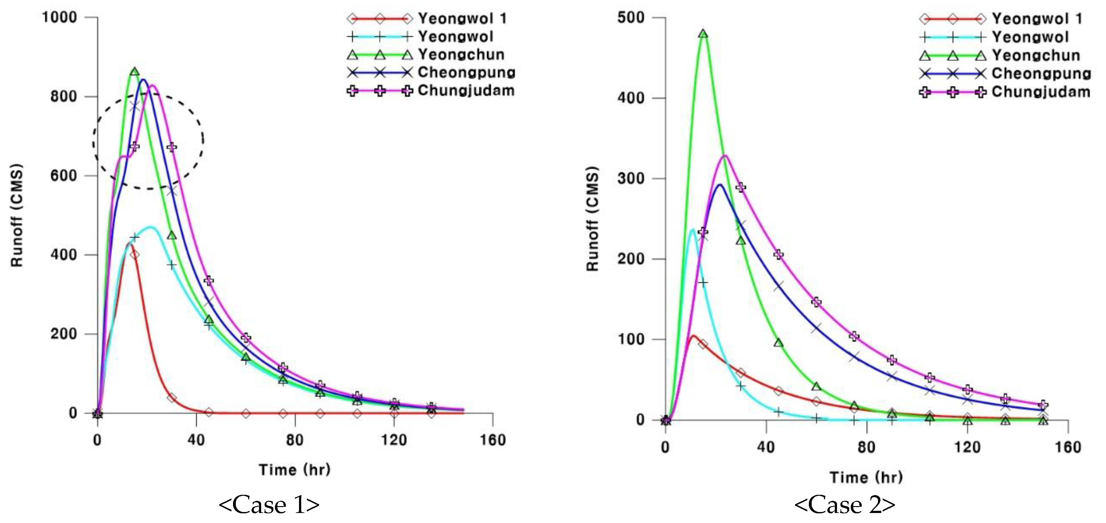
4.2. Development of Unit Hydrographs by Gauge Station
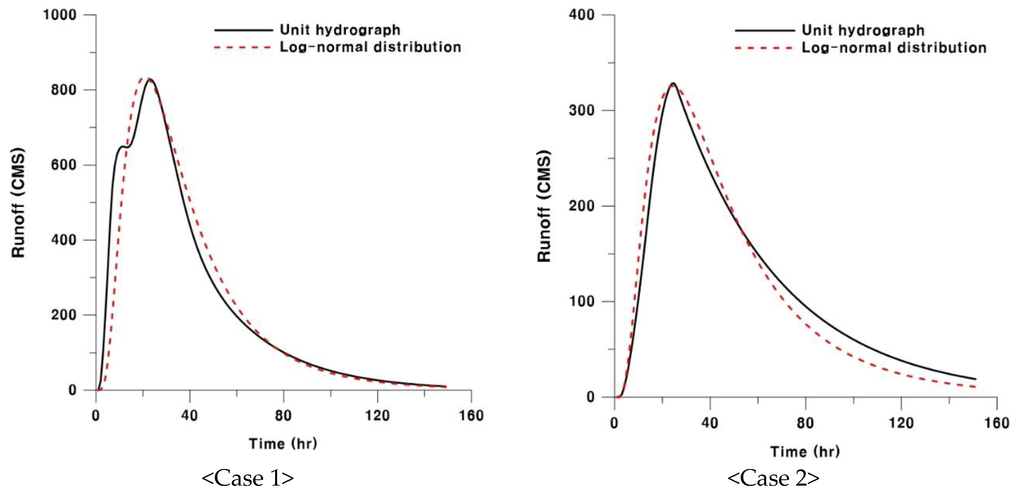
4.3. Conversion of the Developed Unit Hydrograph to the Probability Density Function
5. Application of the Entropy Theory and Construction of an Optimal Stream Gauge Network
- □
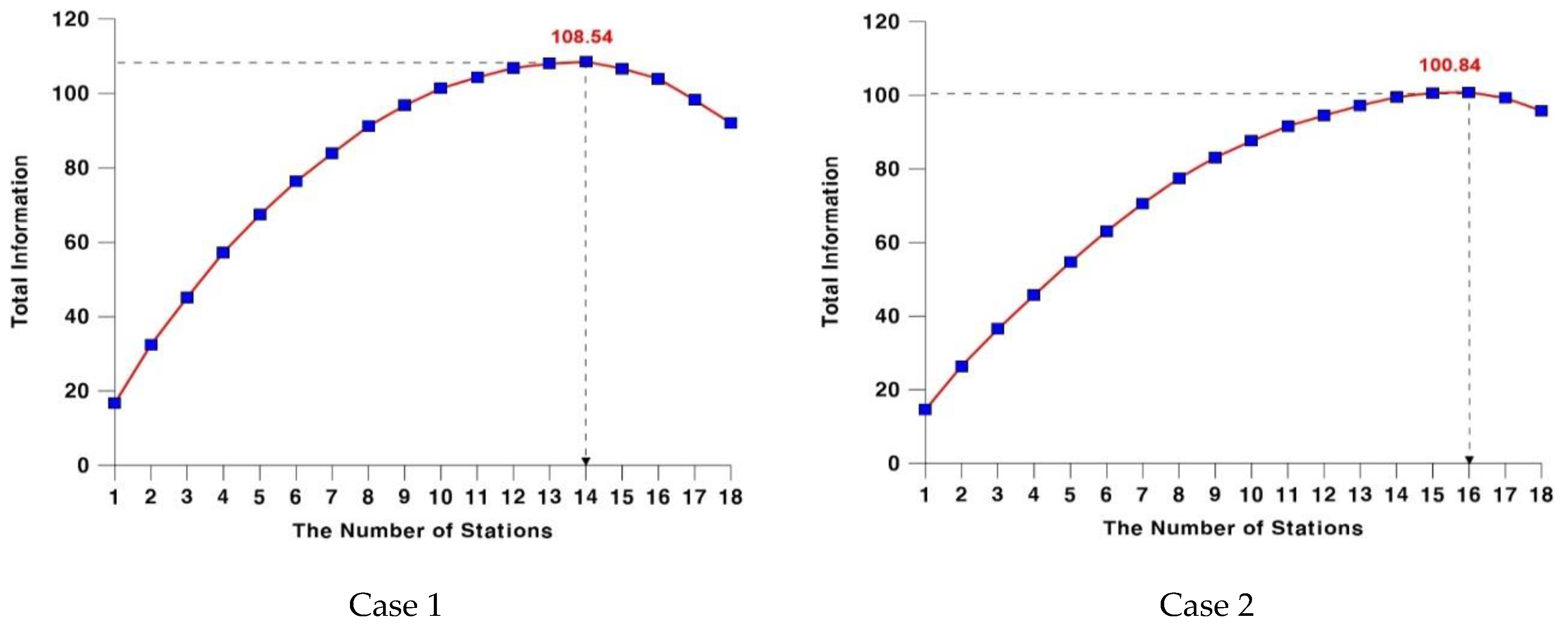
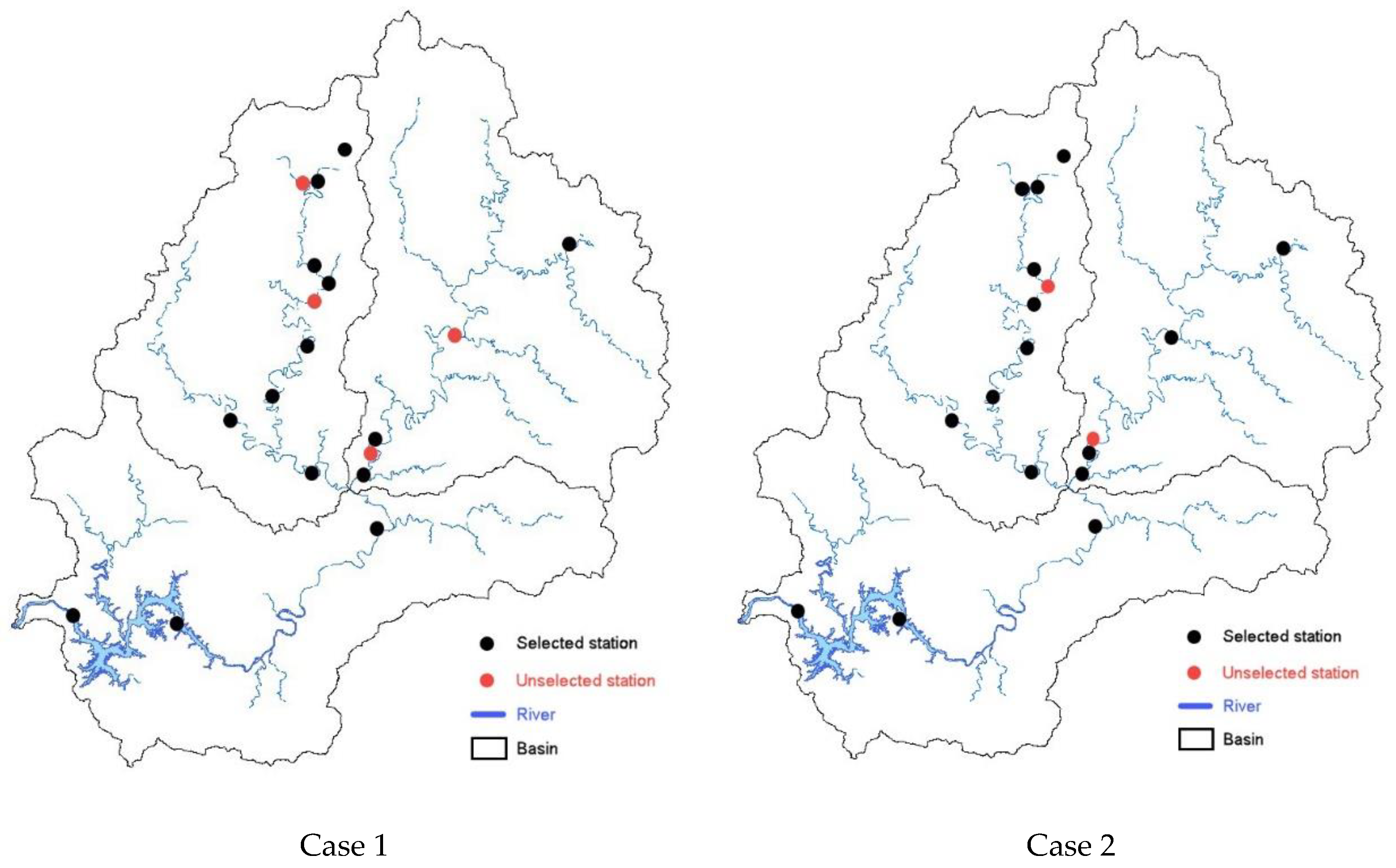
- Case 1
- □
- Case 2
6. Conclusions
Author Contributions
Funding
Conflicts of Interest
References
- Sauer, V.B.; Turnipseed, D.P. Stage Measurement at Gaging Stations: U.S. Geological Survey Techniques and Methods, Chapter 7 of Book 3, Section A.; U.S. Geological Survey: Leston, VA, USA, 2010.
- Osei, M.A.; Amekudzi, L.K.; Wemegah, D.D.; Preko, K.; Gyawu, E.S.; Obiri-Danso, K. Hydro-Climatic Modelling of an Ungauged Basin in Kumasi, Ghana. Hydrol. Earth Syst. Sci. 2018, 1–21. [Google Scholar] [CrossRef]
- Lee, J.H.; Jun, H.D. Evaluation of raingauge network using area average rainfall estimation and the estimation error. J. Wetl. Res. 2014, 16, 103–112. [Google Scholar] [CrossRef]
- Caselton, W.F.; Husain, T. Hydrologic networks: Information transmission. J. Water Resour. Plan. Manag. 1980, 106, 503–529. [Google Scholar]
- Chapman, T.G. Entropy as a measurement of hydrologic data uncertainty and model performance. J. Hydrol. 1986, 85, 111–126. [Google Scholar] [CrossRef]
- Krstanovic, P.F.; Singh, V.P. Evaluation of rainfall networks using entropy: II. Application. Water Resour. Manag. 1992, 6, 295–314. [Google Scholar] [CrossRef]
- Al-Zahrani, M.; Husain, T. An algorithm for designing a precipitation network in the south-western region of Saudi Arabia. J. Hydrol. 1998, 205, 205–216. [Google Scholar] [CrossRef]
- Markus, M.; Knapp, H.V.; Tasker, G.D. Entropy and generalized least square methods in assessment of regional value of stream gages. J. Hydrol. 2003, 283, 107–121. [Google Scholar] [CrossRef]
- Yang, Y.; Burn, D.H. An entropy approach to data collection network design. J. Hydrol. Eng. 1994, 157, 307–324. [Google Scholar] [CrossRef]
- Kim, J.B.; Bae, Y.D.; Park, B.J.; Kim, J.H. Evaluation of the soundness of the raingauge network in the Soyang-dam basin. In Proceedings of the Korea Water Resources Association Annual Conference, Korea, 17 May 2007; pp. 178–182. [Google Scholar]
- Lee, J.H.; Byun, H.; Kim, H.S.; Jun, H.D. Evaluation of a raingauge network considering the spatial distribution characteristics and entropy: A case study of Imha dam basin. J. Korean Soc. Hazard Mitig. 2013, 13, 217–226. [Google Scholar] [CrossRef]
- Singh, V.P. Entropy-Based Parameter Estimation in Hydrology; Springer: Berlin/Heidelberg, Germany, 1998. [Google Scholar]
- Chou, C.M. Applying Multiscale Entropy to the Complexity Analysis of Rainfall-Runoff Relationships. Entropy 2012, 14, 945–957. [Google Scholar] [CrossRef]
- Zhu, Q.; Shen, L.; Liu, P.; Zhao, Y.; Yang, Y.; Huang, D.; Wang, P.; Yang, J. Evolution of the Water Resources System Based on Synergetic and Entropy Theory. Pol. J. Environ. Stud. 2015, 24, 2727–2738. [Google Scholar] [CrossRef]
- Wrzesiński, D. Uncertainty of flow regime characteristics of rivers in Europe. Quaest. Geogr. 2013, 32, 49–59. [Google Scholar] [CrossRef]
- Wrzesiński, D. Use of entropy in the assessment of uncertainty of river runoff regime in Poland. Acta Geophys. 2016, 64, 1825–1839. [Google Scholar] [CrossRef]
- Faiz, M.A.; Liu, D.; Fu, Q.; Wrzesiński, D.; Muneer, S.; Khan, M.I.; Li, T.; Cui, S. Assessment of precipitation variability and uncertainty of stream flow in the Hindu Kush Himalayan and Karakoram River basins of Pakistan. Meteorol. Atmos. Phys. 2019, 131, 127–136. [Google Scholar] [CrossRef]
- Wang, K.; Chen, N.; Tong, D.; Wang, K.; Gong, J. Optimizing the configuration of streamflow stations based on coverage maximization: A case study of the Jinsha River Basin. J. Hydrol. 2015, 527, 172–183. [Google Scholar] [CrossRef]
- Yu, Y.; Zhang, H.; Singh, V.P. Forward Prediction of Runoff Data in Data-Scarce Basins with an Improved Ensemble Empirical Mode Decomposition (EEMD) Model. Water 2018, 10, 388. [Google Scholar] [CrossRef]
- Lay-Ekuakille, A.; Telesca, V.; Ragosta, M.; Giorgio, G.A.; Mvemba, P.K.; Kidiamboko, S. Supervised and characterized smart monitoring network for sensing environmental quantities. IEEE Sens. J. 2017, 17, 7812–7819. [Google Scholar] [CrossRef]
- Shannon, C.E.; Weaver, W. The Mathematical Theory of Communication; The University of Illinois Press: Urbana, IL, USA, 1963. [Google Scholar]
- Ozkul, S.; Harmancioglu, N.B.; Singh, V.P. Entropy-based assessment of water quality monitoring networks. J. Hydrol. Eng. 2000, 5, 90–100. [Google Scholar] [CrossRef]
- World Meteorological Organization (WMO). Guide to Hydrological Practices, 5th ed.; WMO: Geneva, Switzerland, 2008. [Google Scholar]
- Lee, J.H.; Kim, S.J.; Jun, H.D. A Study of the Influence of the Spatial Distribution of Rain Gauge Networks on Areal Average Rainfall Calculation. Water 2018, 10, 1635. [Google Scholar] [CrossRef]
- Clark, C.O. Storage and the unit hydrograph. Trans. Am. Soc. Civ. Eng. 1945, 110, 1419–1446. [Google Scholar]
- Yoo, C.S.; Ku, H.J.; Kim, K.W. Use of a Distance Measure for the Comparison of Unit Hydrographs: Application to the Stream Gauge Network Optimization. J. Hydrol. Eng. 2001, 16, 880–890. [Google Scholar] [CrossRef]
- Lee, J.H.; Yoo, C.S. Decision of basin representative concentration time and storage coefficient considering antecedent moisture conditions. J. Korean Soc. Hazard Mitig. 2011, 11, 255–264. [Google Scholar] [CrossRef]
- Zhang, L.; Singh, V.P. Bivariate rainfall and runoff analysis using entropy and copula theories. Entropy 2012, 14, 1784–1812. [Google Scholar] [CrossRef]
- Guo, A.; Chang, J.; Wang, Y.; Huang, Q.; Guo, Z. Maximum Entropy-Copula Method for Hydrological Risk Analysis under Uncertainty: A Case Study on the Loess Plateau, China. Entropy 2017, 19, 609. [Google Scholar] [CrossRef]

| Basin | No. of Stream Gauge Station | Name of Stream Gauge Station | Basin Area (km2) | Stream Length (km) | Stream Slope | Density | |
|---|---|---|---|---|---|---|---|
| (km2/# R.G.) | (#R.G./km2) | ||||||
| Namhan River Basin | 1 | Imgye | 457.5 | 7.5 | 0.01042 | 457.5 | 0.0022 |
| 2 | Jeongseon 2 | 1682.1 | 93.1 | 0.00569 | 841.1 | 0.0012 | |
| 3 | Geoun | 2272.1 | 142.2 | 0.00297 | 757.4 | 0.0013 | |
| 4 | Yeongwol 2 | 2287.9 | 147.8 | 0.00263 | 572.0 | 0.0017 | |
| 5 | Yeongwol | 2447.8 | 153.4 | 0.00254 | 489.6 | 0.0020 | |
| Pyeongchang River Basin | 6 | Imokjeong | 54.3 | 7.5 | 0.01604 | 54.3 | 0.0184 |
| 7 | Jangpyeonggyo | 104.5 | 24.3 | 0.01214 | 52.3 | 0.0191 | |
| 8 | Baekokpo | 143.6 | 21.8 | 0.00590 | 47.9 | 0.0209 | |
| 9 | Sanganmi | 394.8 | 49.3 | 0.00790 | 98.7 | 0.0101 | |
| 10 | Habanjeong | 81.4 | 16.7 | 0.01420 | 81.4 | 0.0123 | |
| 11 | Bangrimgyo | 524.2 | 54.3 | 0.00726 | 104.8 | 0.0095 | |
| 12 | Pyeongchang | 695.6 | 76.9 | 0.00513 | 115.9 | 0.0086 | |
| 13 | Panun | 830.1 | 101.2 | 0.00348 | 118.6 | 0.0084 | |
| 14 | Jucheon | 528.8 | 73.2 | 0.00436 | 528.8 | 0.0019 | |
| 15 | Yeongwol 1 | 1399.6 | 136.5 | 0.00250 | 140.0 | 0.0714 | |
| After confluence of Namhan and Pyeongchang River Basin | - | - | 3847.0 | - | - | 256.5 | 0.0039 |
| Chungju Dam Basin | 16 | Yeongchun | 4543.4 | 181.5 | 0.00162 | 285.0 | 0.0035 |
| 17 | Cheongpung | 5388.1 | 240.7 | 0.00126 | 316.9 | 0.0032 | |
| 18 | Chungju Dam | 6648.0 | 268.2 | 0.00126 | 369.3 | 0.0027 | |
| Total | - | - | 6648.0 | - | - | 369.3 | 0.0027 |
| Physiographic Unit | Streamflow |
|---|---|
| Coastal | 2750 |
| Mountains | 1000 |
| Interior plains | 1875 |
| Hilly/undulating | 1875 |
| Small islands | 300 |
| Polar/arid | 20,000 |
| # Event | Date (Y/M/D/H) | Total Rainfall (mm) | Rainfall Duration (hr) | Total Five-Day Antecedent Rainfall (mm) | AMC | Maximum Rainfall Intensity (mm/hr) | Average Rainfall Intensity (mm/hr) | Centroid of Hyetograph (hr) |
|---|---|---|---|---|---|---|---|---|
| 1 | 2008/07/23/10 | 220.4 | 92 | 141.4 | III | 15.62 | 2.40 | 32.6 |
| 2 | 2010/09/09/14 | 182.2 | 98 | 142.3 | III | 17.08 | 1.86 | 52.3 |
| Basin | Number of Stream Gauge Station | Name of Stream Gauge Station | Case 1 | Case 2 | ||
|---|---|---|---|---|---|---|
| Average | SD | Average | SD | |||
| Namhan River basin | 1 | Imgye | 1.43 | 0.44 | 0.92 | 0.18 |
| 2 | Jeongseon 2 | 2.15 | 0.41 | 1.77 | 0.53 | |
| 3 | Geoun | 2.55 | 0.36 | 2.68 | 0.62 | |
| 4 | Yeongwol 2 | 2.59 | 0.35 | 2.82 | 0.68 | |
| 5 | Yeongwol | 2.58 | 0.36 | 2.58 | 0.57 | |
| Pyeongchang River basin | 6 | Imokjeong | 1.47 | 0.40 | 1.00 | 0.28 |
| 7 | Jangpyeonggyo | 1.62 | 0.40 | 0.62 | 0.46 | |
| 8 | Baekokpo | 1.51 | 0.39 | 0.72 | 0.44 | |
| 9 | Sanganmi | 1.74 | 0.38 | 1.19 | 0.50 | |
| 10 | Habanjeong | 1.81 | 0.46 | 0.97 | 0.24 | |
| 11 | Bangrimgyo | 1.80 | 0.41 | 1.23 | 0.48 | |
| 12 | Pyeongchang | 2.03 | 0.40 | 1.96 | 0.61 | |
| 13 | Panun | 2.23 | 0.37 | 2.73 | 0.68 | |
| 14 | Jucheon | 2.00 | 0.53 | 2.10 | 0.63 | |
| 15 | Yeongwol 1 | 2.35 | 0.44 | 3.32 | 0.71 | |
| Chungju Dam basin | 16 | Yeongchun | 2.54 | 0.43 | 3.05 | 0.58 |
| 17 | Cheongpung | 2.83 | 0.38 | 3.75 | 0.64 | |
| 18 | Chungjudam | 3.57 | 0.25 | 3.80 | 0.63 | |
| 1 | 2 | 3 | 4 | 5 | 6 | 7 | 8 | 9 | 10 | 11 | 12 | 13 | 14 | 15 | 16 | 17 | 18 | |
| 1 | 5.203 | 0.106 | 0.001 | 0.000 | 0.000 | 2.171 | 1.059 | 1.672 | 0.605 | 0.600 | 0.528 | 0.185 | 0.047 | 0.372 | 0.039 | 0.005 | 0.003 | 0.005 |
| 2 | 0.106 | 5.133 | 0.341 | 0.264 | 0.293 | 0.120 | 0.252 | 0.146 | 0.426 | 0.566 | 0.555 | 1.558 | 1.628 | 1.008 | 1.124 | 0.480 | 0.072 | 0.036 |
| 3 | 0.001 | 0.341 | 5.002 | 2.339 | 2.754 | 0.001 | 0.008 | 0.001 | 0.024 | 0.056 | 0.045 | 0.185 | 0.502 | 0.169 | 0.808 | 1.900 | 0.632 | 0.427 |
| 4 | 0.000 | 0.264 | 2.339 | 4.974 | 3.318 | 0.000 | 0.004 | 0.000 | 0.013 | 0.038 | 0.028 | 0.137 | 0.392 | 0.130 | 0.651 | 1.514 | 0.770 | 0.525 |
| 5 | 0.000 | 0.293 | 2.754 | 3.318 | 5.002 | 0.000 | 0.005 | 0.001 | 0.017 | 0.045 | 0.035 | 0.155 | 0.432 | 0.145 | 0.709 | 1.681 | 0.732 | 0.499 |
| 6 | 2.171 | 0.120 | 0.001 | 0.000 | 0.000 | 5.108 | 1.332 | 2.516 | 0.731 | 0.692 | 0.623 | 0.213 | 0.053 | 0.414 | 0.044 | 0.006 | 0.003 | 0.005 |
| 7 | 1.059 | 0.252 | 0.008 | 0.004 | 0.005 | 1.332 | 5.108 | 1.652 | 1.446 | 1.248 | 1.179 | 0.420 | 0.132 | 0.695 | 0.106 | 0.025 | 0.001 | 0.003 |
| 8 | 1.672 | 0.146 | 0.001 | 0.000 | 0.001 | 2.516 | 1.652 | 5.083 | 0.874 | 0.803 | 0.736 | 0.255 | 0.067 | 0.471 | 0.054 | 0.009 | 0.003 | 0.005 |
| 9 | 0.605 | 0.426 | 0.024 | 0.013 | 0.017 | 0.731 | 1.446 | 0.874 | 5.057 | 1.921 | 2.275 | 0.701 | 0.241 | 1.000 | 0.188 | 0.056 | 0.000 | 0.001 |
| 10 | 0.600 | 0.566 | 0.056 | 0.038 | 0.045 | 0.692 | 1.248 | 0.803 | 1.921 | 5.248 | 2.488 | 0.883 | 0.344 | 1.402 | 0.277 | 0.102 | 0.003 | 0.000 |
| 11 | 0.528 | 0.555 | 0.045 | 0.028 | 0.035 | 0.623 | 1.179 | 0.736 | 2.275 | 2.488 | 5.133 | 0.900 | 0.329 | 1.277 | 0.258 | 0.088 | 0.001 | 0.000 |
| 12 | 0.185 | 1.558 | 0.185 | 0.137 | 0.155 | 0.213 | 0.420 | 0.255 | 0.701 | 0.883 | 0.900 | 5.108 | 0.926 | 1.411 | 0.680 | 0.281 | 0.027 | 0.010 |
| 13 | 0.047 | 1.628 | 0.502 | 0.392 | 0.432 | 0.053 | 0.132 | 0.067 | 0.241 | 0.344 | 0.329 | 0.926 | 5.030 | 0.650 | 1.584 | 0.670 | 0.112 | 0.059 |
| 14 | 0.372 | 1.008 | 0.169 | 0.130 | 0.145 | 0.414 | 0.695 | 0.471 | 1.000 | 1.402 | 1.277 | 1.411 | 0.650 | 5.389 | 0.554 | 0.252 | 0.034 | 0.015 |
| 15 | 0.039 | 1.124 | 0.808 | 0.651 | 0.709 | 0.044 | 0.106 | 0.054 | 0.188 | 0.277 | 0.258 | 0.680 | 1.584 | 0.554 | 5.203 | 1.095 | 0.237 | 0.150 |
| 16 | 0.005 | 0.480 | 1.900 | 1.514 | 1.681 | 0.006 | 0.025 | 0.009 | 0.056 | 0.102 | 0.088 | 0.281 | 0.670 | 0.252 | 1.095 | 5.180 | 0.577 | 0.396 |
| 17 | 0.003 | 0.072 | 0.632 | 0.770 | 0.732 | 0.003 | 0.001 | 0.003 | 0.000 | 0.003 | 0.001 | 0.027 | 0.112 | 0.034 | 0.237 | 0.577 | 5.057 | 1.890 |
| 18 | 0.005 | 0.036 | 0.427 | 0.525 | 0.499 | 0.005 | 0.003 | 0.005 | 0.001 | 0.000 | 0.000 | 0.010 | 0.059 | 0.015 | 0.150 | 0.396 | 1.890 | 5.002 |
| 1 | 2 | 3 | 4 | 5 | 6 | 7 | 8 | 9 | 10 | 11 | 12 | 13 | 14 | 15 | 16 | 17 | 18 | |
| 1 | 4.331 | 0.060 | 0.001 | 0.001 | 0.001 | 1.176 | 0.258 | 0.373 | 0.467 | 1.575 | 0.433 | 0.041 | 0.000 | 0.022 | 0.010 | 0.005 | 0.024 | 0.026 |
| 2 | 0.060 | 5.389 | 0.145 | 0.112 | 0.170 | 0.129 | 0.035 | 0.055 | 0.379 | 0.100 | 0.432 | 1.577 | 0.163 | 1.042 | 0.001 | 0.006 | 0.093 | 0.116 |
| 3 | 0.001 | 0.145 | 5.546 | 2.053 | 2.266 | 0.000 | 0.002 | 0.001 | 0.005 | 0.000 | 0.006 | 0.283 | 2.757 | 0.430 | 0.423 | 0.648 | 0.004 | 0.000 |
| 4 | 0.001 | 0.112 | 2.053 | 5.638 | 1.472 | 0.000 | 0.003 | 0.002 | 0.002 | 0.001 | 0.003 | 0.225 | 2.223 | 0.343 | 0.587 | 0.870 | 0.021 | 0.004 |
| 5 | 0.001 | 0.170 | 2.266 | 1.472 | 5.462 | 0.000 | 0.002 | 0.001 | 0.006 | 0.000 | 0.007 | 0.327 | 1.917 | 0.495 | 0.321 | 0.504 | 0.000 | 0.006 |
| 6 | 1.176 | 0.129 | 0.000 | 0.000 | 0.000 | 4.742 | 0.328 | 0.477 | 0.884 | 2.198 | 0.828 | 0.087 | 0.000 | 0.051 | 0.014 | 0.008 | 0.040 | 0.043 |
| 7 | 0.258 | 0.035 | 0.002 | 0.003 | 0.002 | 0.328 | 5.248 | 1.942 | 0.380 | 0.296 | 0.305 | 0.025 | 0.001 | 0.013 | 0.018 | 0.009 | 0.043 | 0.047 |
| 8 | 0.373 | 0.055 | 0.001 | 0.002 | 0.001 | 0.477 | 1.942 | 5.203 | 0.515 | 0.434 | 0.420 | 0.038 | 0.001 | 0.021 | 0.018 | 0.009 | 0.046 | 0.049 |
| 9 | 0.467 | 0.379 | 0.005 | 0.002 | 0.006 | 0.884 | 0.380 | 0.515 | 5.331 | 0.698 | 2.566 | 0.266 | 0.008 | 0.177 | 0.015 | 0.007 | 0.078 | 0.086 |
| 10 | 1.575 | 0.100 | 0.000 | 0.001 | 0.000 | 2.198 | 0.296 | 0.434 | 0.698 | 4.589 | 0.655 | 0.067 | 0.000 | 0.039 | 0.012 | 0.007 | 0.033 | 0.036 |
| 11 | 0.433 | 0.432 | 0.006 | 0.003 | 0.007 | 0.828 | 0.305 | 0.420 | 2.566 | 0.655 | 5.290 | 0.299 | 0.010 | 0.199 | 0.014 | 0.006 | 0.078 | 0.086 |
| 12 | 0.041 | 1.577 | 0.283 | 0.225 | 0.327 | 0.087 | 0.025 | 0.038 | 0.266 | 0.067 | 0.299 | 5.530 | 0.306 | 1.871 | 0.014 | 0.034 | 0.078 | 0.107 |
| 13 | 0.000 | 0.163 | 2.757 | 2.223 | 1.917 | 0.000 | 0.001 | 0.001 | 0.008 | 0.000 | 0.010 | 0.306 | 5.638 | 0.456 | 0.449 | 0.665 | 0.006 | 0.000 |
| 14 | 0.022 | 1.042 | 0.430 | 0.343 | 0.495 | 0.051 | 0.013 | 0.021 | 0.177 | 0.039 | 0.199 | 1.871 | 0.456 | 5.562 | 0.038 | 0.074 | 0.058 | 0.088 |
| 15 | 0.010 | 0.001 | 0.423 | 0.587 | 0.321 | 0.014 | 0.018 | 0.018 | 0.015 | 0.012 | 0.014 | 0.014 | 0.449 | 0.038 | 5.682 | 1.446 | 0.328 | 0.229 |
| 16 | 0.005 | 0.006 | 0.648 | 0.870 | 0.504 | 0.008 | 0.009 | 0.009 | 0.007 | 0.007 | 0.006 | 0.034 | 0.665 | 0.074 | 1.446 | 5.479 | 0.154 | 0.094 |
| 17 | 0.024 | 0.093 | 0.004 | 0.021 | 0.000 | 0.040 | 0.043 | 0.046 | 0.078 | 0.033 | 0.078 | 0.078 | 0.006 | 0.058 | 0.328 | 0.154 | 5.578 | 2.137 |
| 18 | 0.026 | 0.116 | 0.000 | 0.004 | 0.006 | 0.043 | 0.047 | 0.049 | 0.086 | 0.036 | 0.086 | 0.107 | 0.000 | 0.088 | 0.229 | 0.094 | 2.137 | 5.562 |
| Case 1 | Case 2 | ||||
|---|---|---|---|---|---|
| No. of Stations | Optimized Combination of Stream Gauge Stations | Maximum Information Content | No. of Stations | Optimized Combination of Stream Gauge Stations | Maximum Information Content |
| 1 | 10 | 16.72 | 1 | 13 | 14.60 |
| 2 | 5,10 | 32.45 | 2 | 9,13 | 26.46 |
| 3 | 5,8,10 | 45.19 | 3 | 3,9,12 | 36.51 |
| 4 | 2,5,8,10 | 57.29 | 4 | 3,9,10,12 | 45.72 |
| 5 | 5,6,11,14,15 | 67.36 | 5 | 3,4,9,10,12 | 54.72 |
| 6 | 2,5,6,9,10,16 | 76.30 | 6 | 3,4,9,10,12,17 | 63.09 |
| 7 | 2,5,6,7,11,14,16 | 83.89 | 7 | 3,4,8,9,10,12,17 | 70.62 |
| 8 | 2,5,6,7,11,14,16,17 | 91.20 | 8 | 3,4,8,9,10,12,15,18 | 77.51 |
| 9 | 2,3,4,6,7,11,14,15,18 | 96.78 | 9 | 2,3,4,8,9,10,14,15,18 | 83.15 |
| 10 | 1,2,3,4,8,9,10,14,15,18 | 101.40 | 10 | 1,2,3,4,6,7,9,14,15,18 | 87.60 |
| 11 | 1,2,5,8,9,10,14,15,16,17,18 | 104.31 | 11 | 1,2,5,6,7,9,13,14,15,16,18 | 91.65 |
| 12 | 1,3,5,7,8,11,12,13,14,15,17,18 | 106.86 | 12 | 1,2,5,6,7,9,13,14,15,16,17,18 | 94.52 |
| 13 | 1,3,5,6,7,9,10,12,13,14,15,17,18 | 107.99 | 13 | 1,2,5,6,7,8,11,13,14,15,16,17,18 | 97.25 |
| 14 | 1,3,5,6,7,9,10,12,13,14,15,16,17,18 | 108.54 | 14 | 1,2,4,5,6,7,8,11,13,14,15,16,17,18 | 99.53 |
| 15 | 1,2,3,4,6,7,9,10,12,13,14,15,16,17,18 | 106.69 | 15 | 1,2,4,5,6,7,8,11,12,13,14,15,16,17,18 | 100.64 |
| 16 | 1,2,3,4,6,7,8,9,10,12,13,14,15,16,17,18 | 103.98 | 16 | 1,2,4,5,6,7,8,9,11,12,13,14,15,16,17,18 | 100.84 |
| 17 | 1,2,3,4,5,6,7,8,9,11,12,13,14,15,16,17,18 | 98.24 | 17 | 1,2,4,5,6,7,8,9,10,11,12,13,14,15,16,17,18 | 99.28 |
| 18 | 1,2,3,4,5,6,7,8,9,10,11,12,13,14,15,16,17,18 | 92.02 | 18 | 1,2,3,4,5,6,7,8,9,10,11,12,13,14,15,16,17,18 | 95.80 |
© 2019 by the authors. Licensee MDPI, Basel, Switzerland. This article is an open access article distributed under the terms and conditions of the Creative Commons Attribution (CC BY) license (http://creativecommons.org/licenses/by/4.0/).
Share and Cite
Joo, H.; Jun, H.; Lee, J.; Kim, H.S. Assessment of a Stream Gauge Network Using Upstream and Downstream Runoff Characteristics and Entropy. Entropy 2019, 21, 673. https://doi.org/10.3390/e21070673
Joo H, Jun H, Lee J, Kim HS. Assessment of a Stream Gauge Network Using Upstream and Downstream Runoff Characteristics and Entropy. Entropy. 2019; 21(7):673. https://doi.org/10.3390/e21070673
Chicago/Turabian StyleJoo, Hongjun, Hwandon Jun, Jiho Lee, and Hung Soo Kim. 2019. "Assessment of a Stream Gauge Network Using Upstream and Downstream Runoff Characteristics and Entropy" Entropy 21, no. 7: 673. https://doi.org/10.3390/e21070673
APA StyleJoo, H., Jun, H., Lee, J., & Kim, H. S. (2019). Assessment of a Stream Gauge Network Using Upstream and Downstream Runoff Characteristics and Entropy. Entropy, 21(7), 673. https://doi.org/10.3390/e21070673