Using Entropy for Welds Segmentation and Evaluation


Abstract
:1. Introduction
2. Preparation of Input Data for the Neural Network
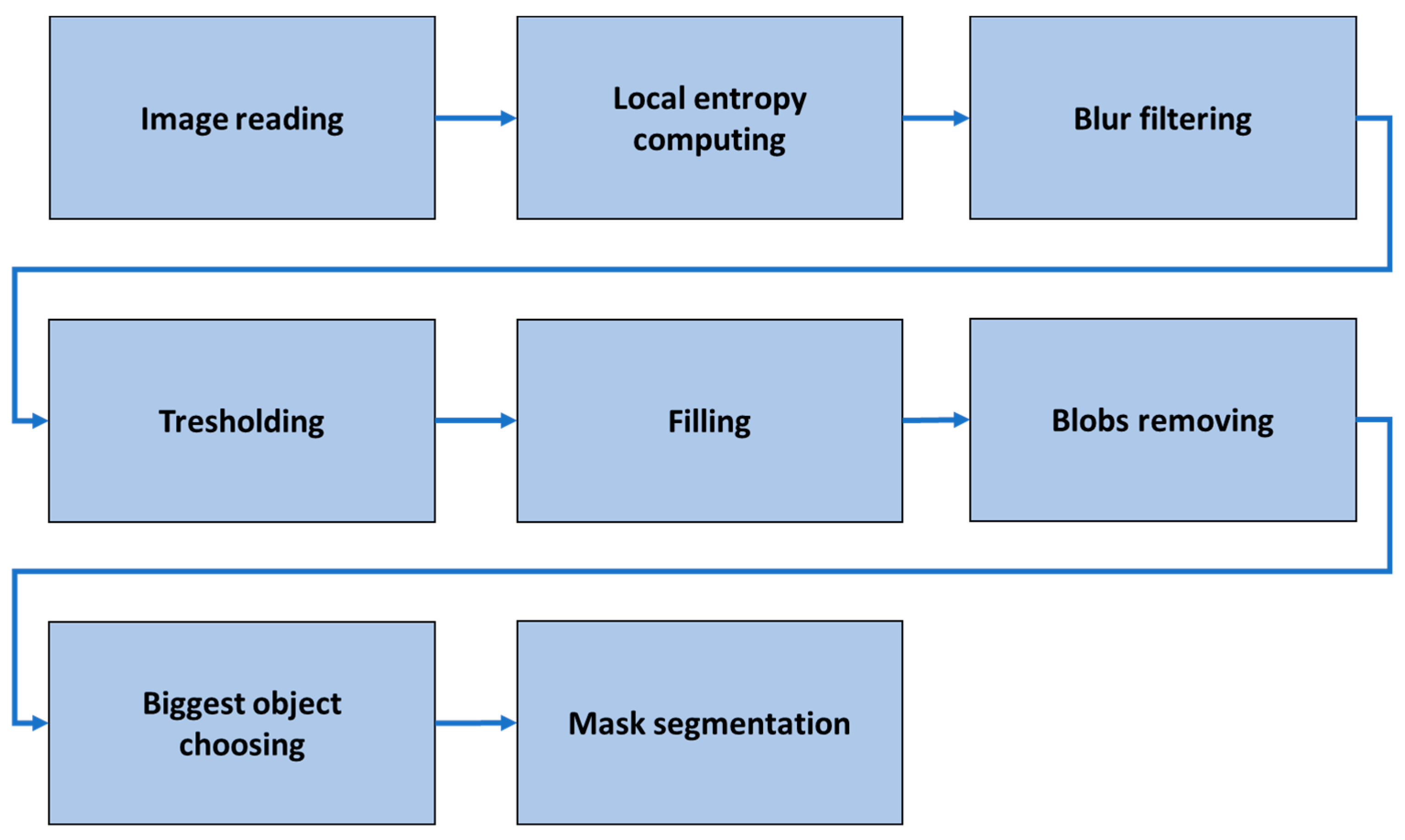
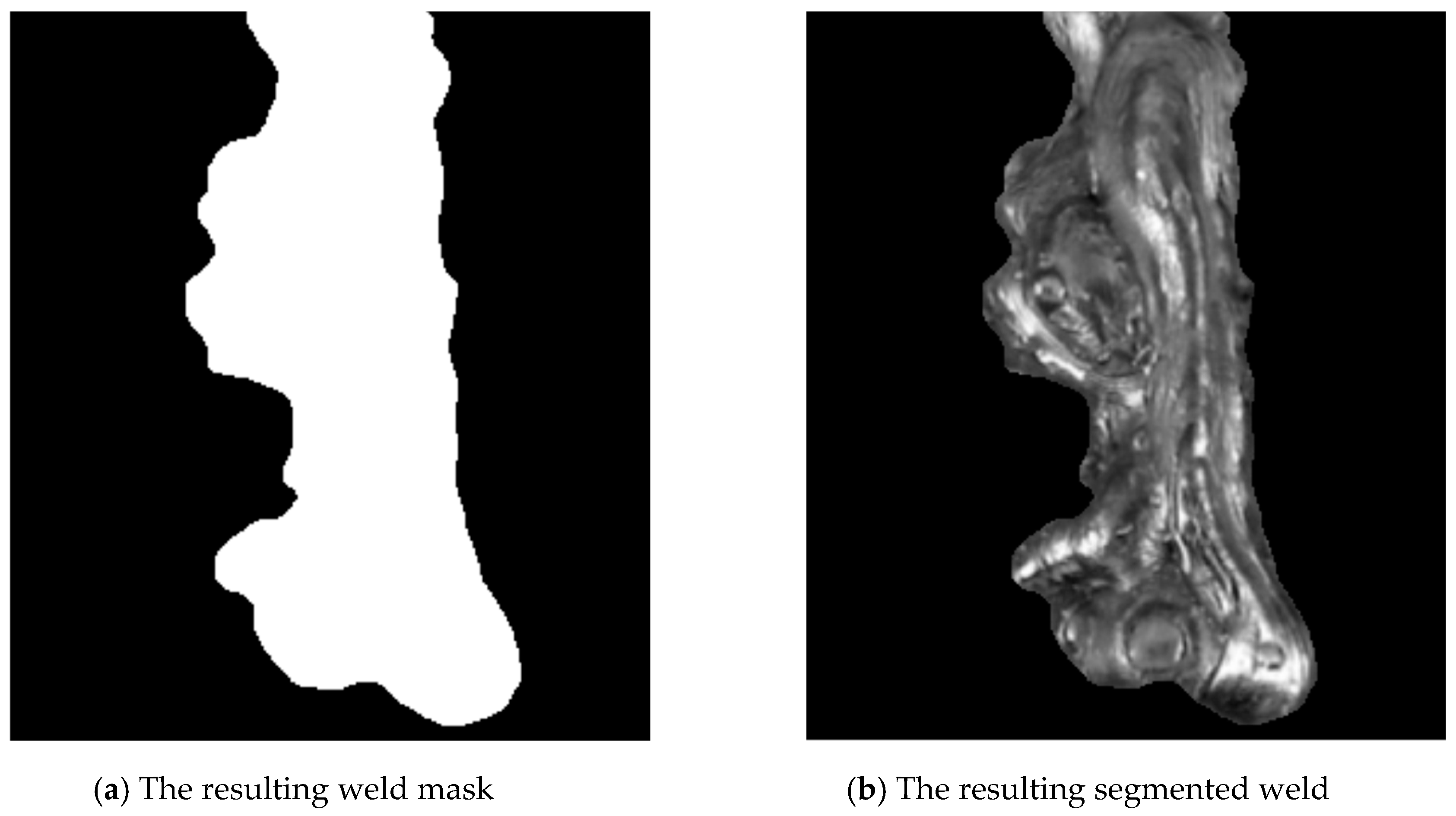
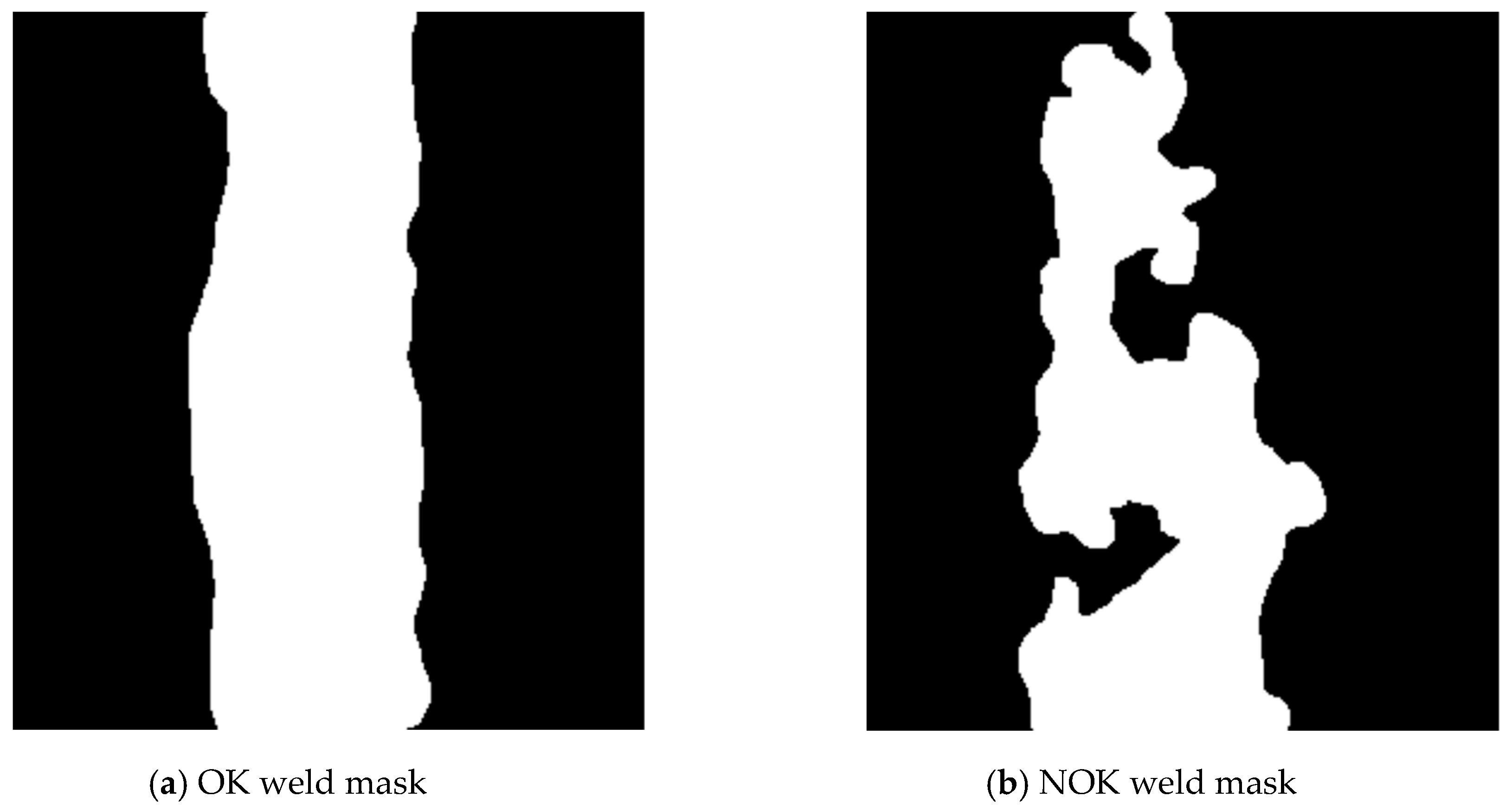
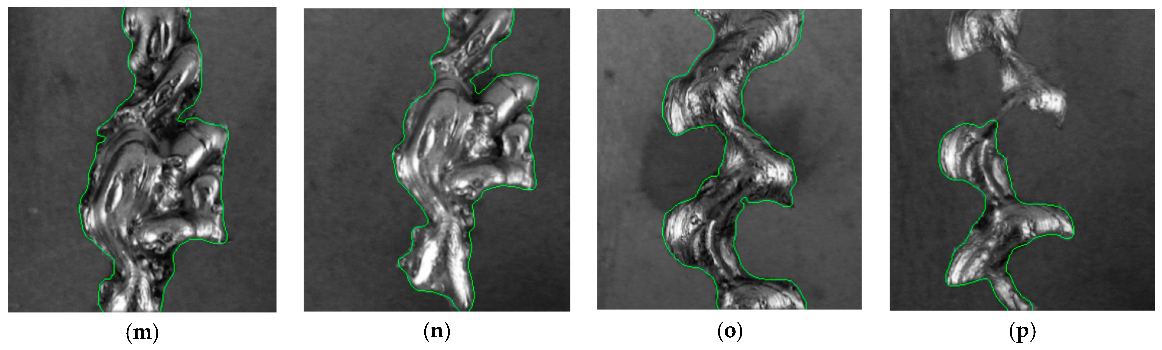
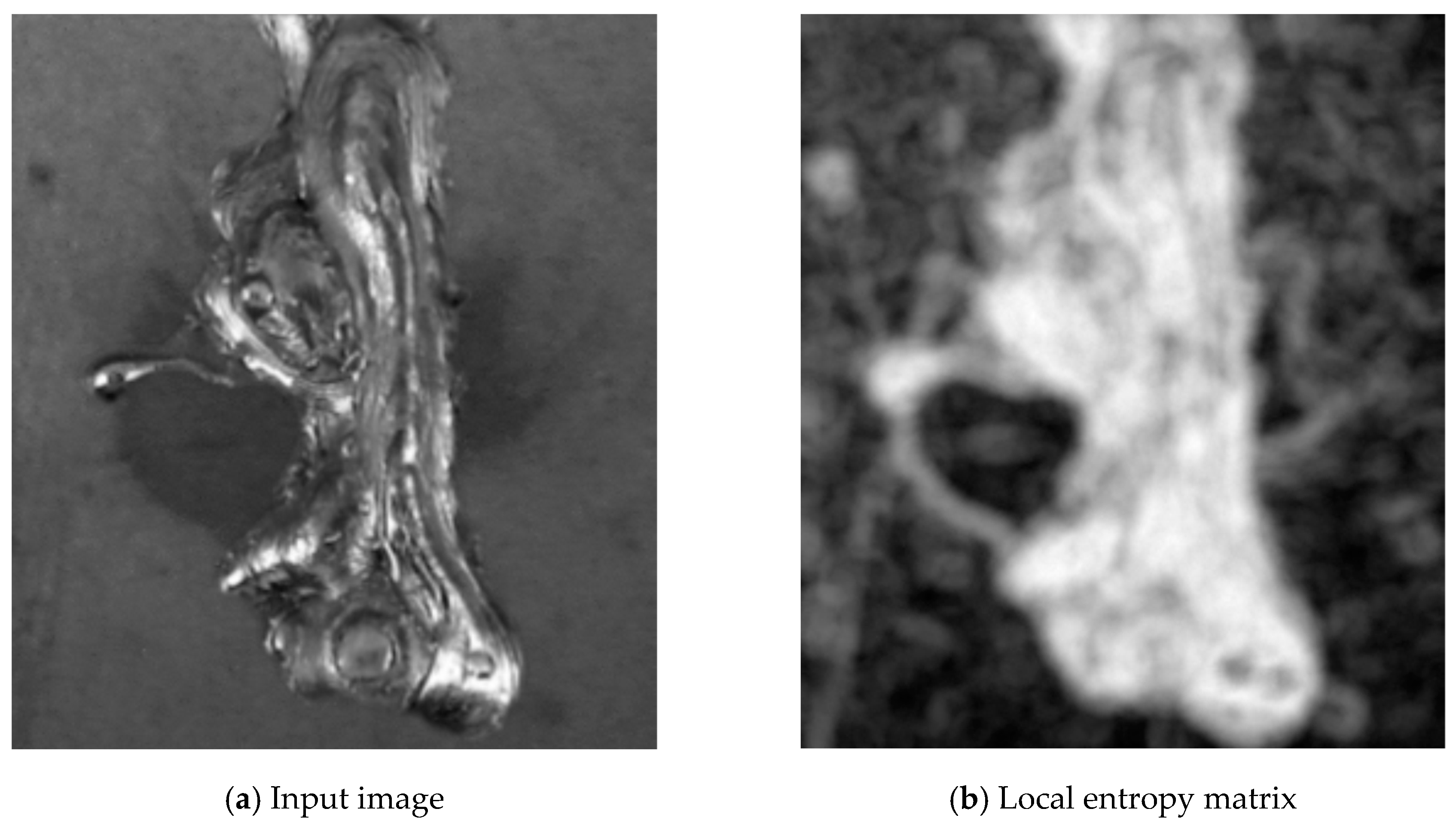
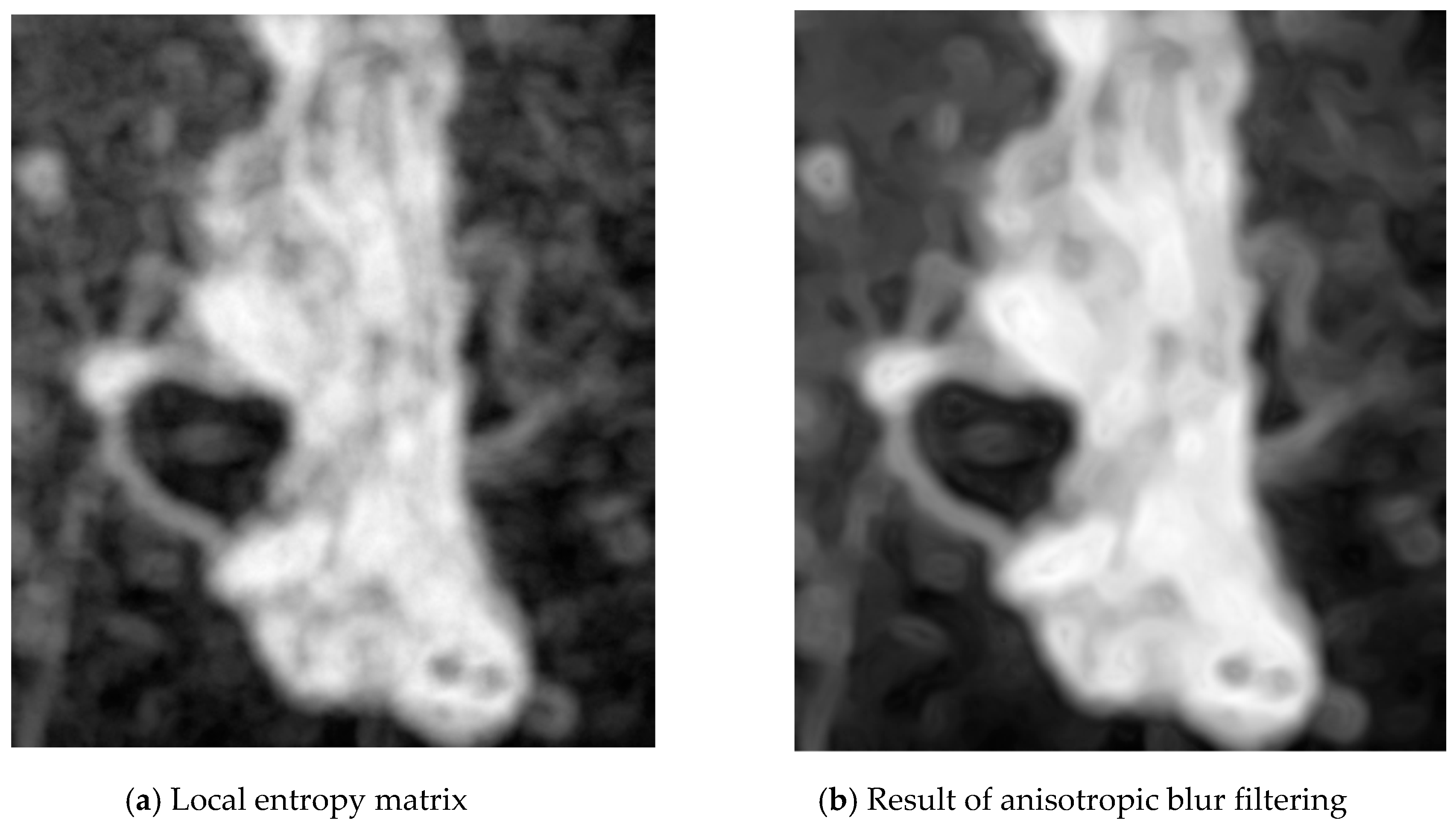
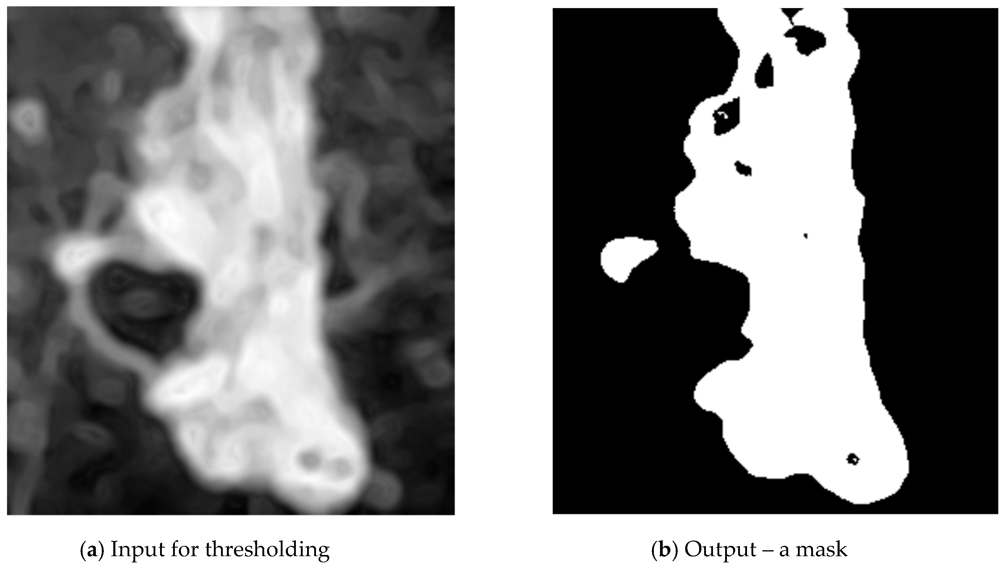
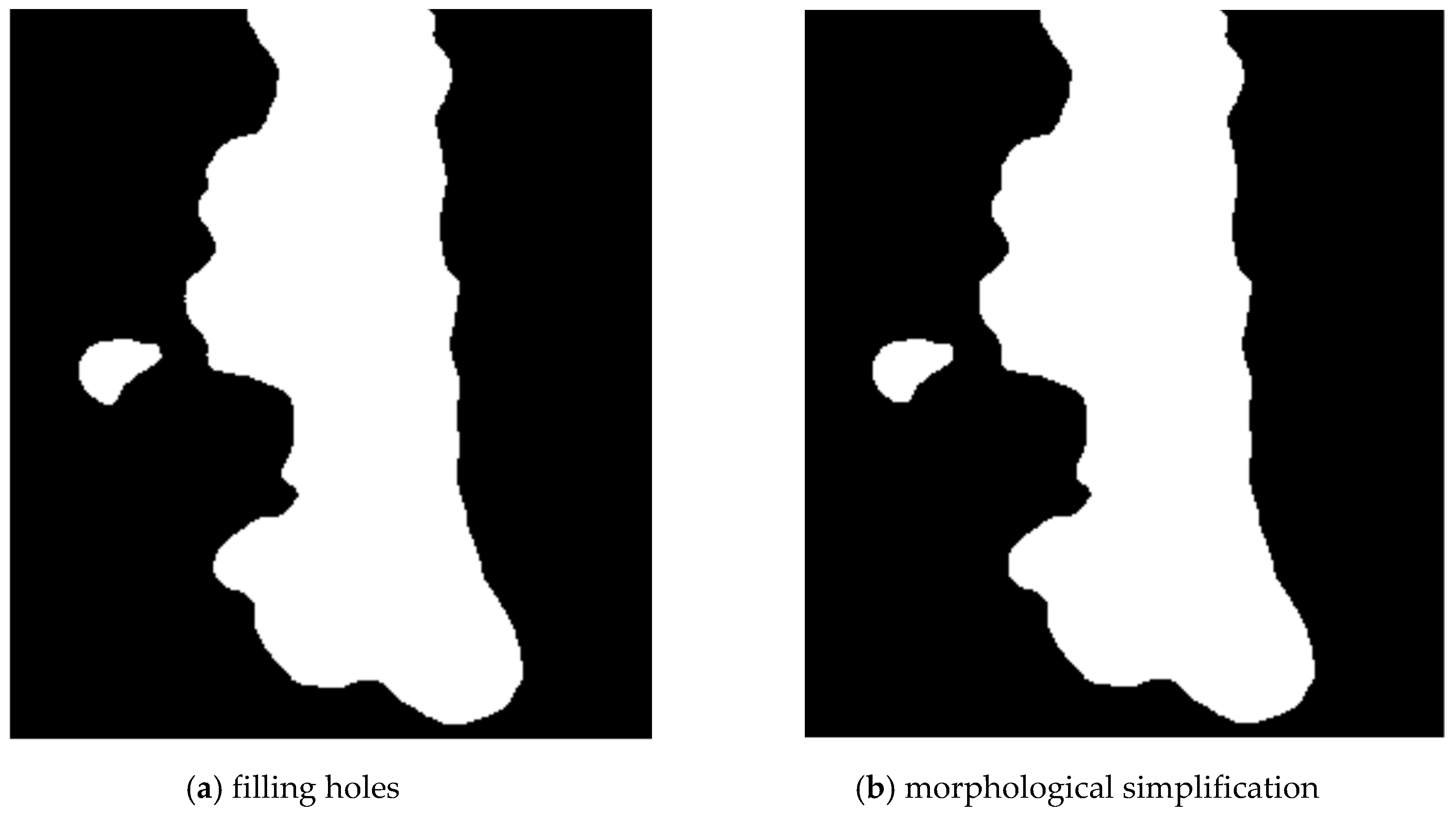
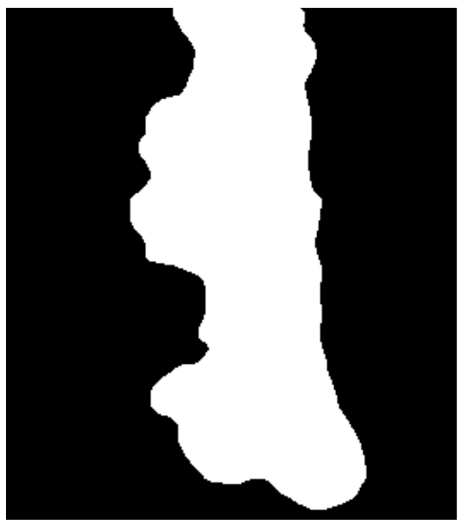
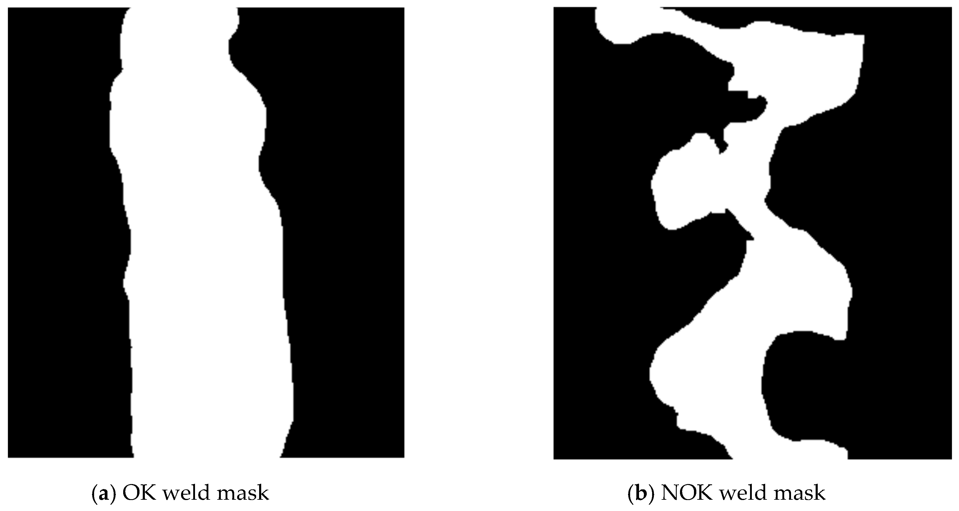
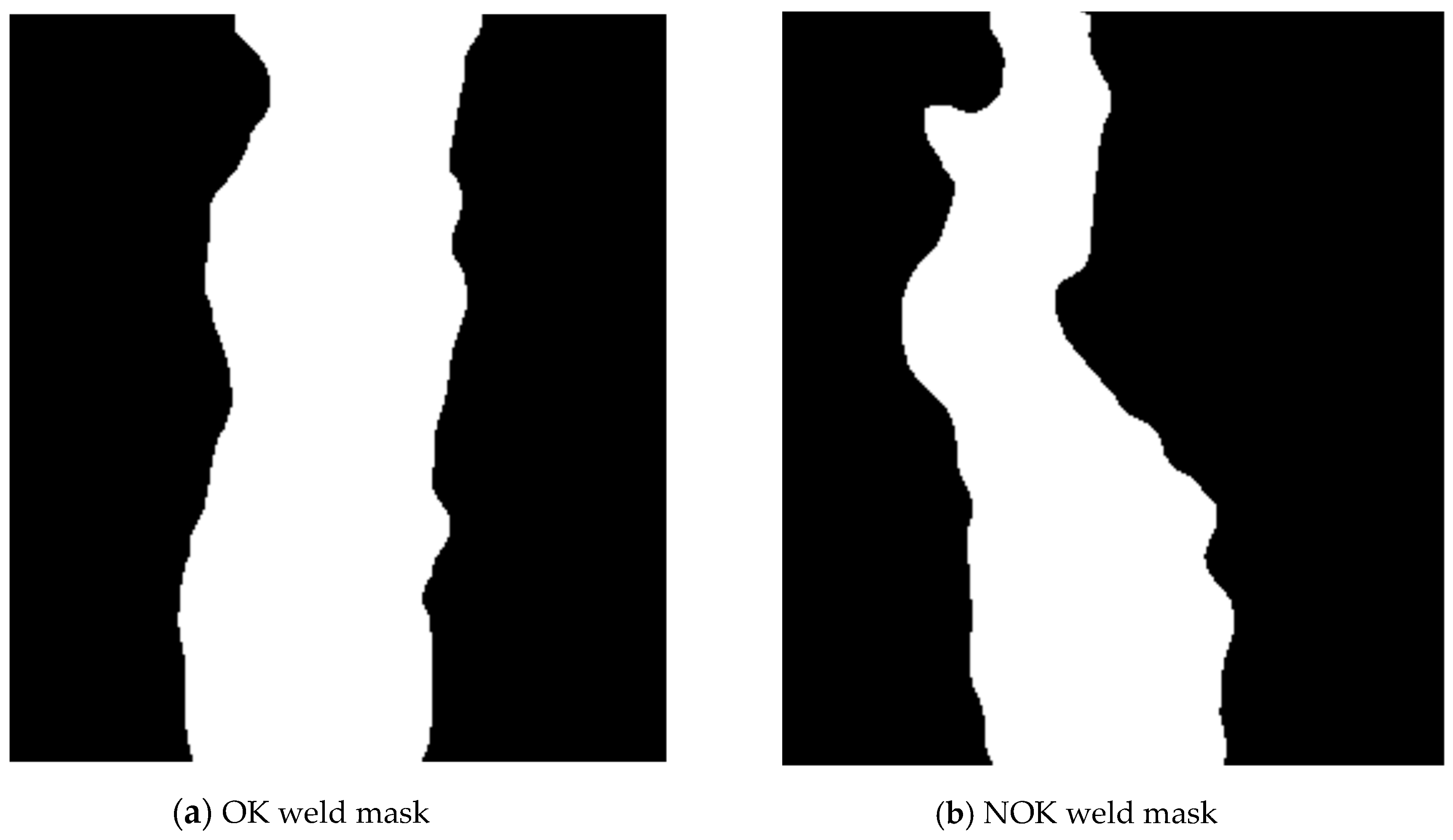
2.1. Weld Segmentation
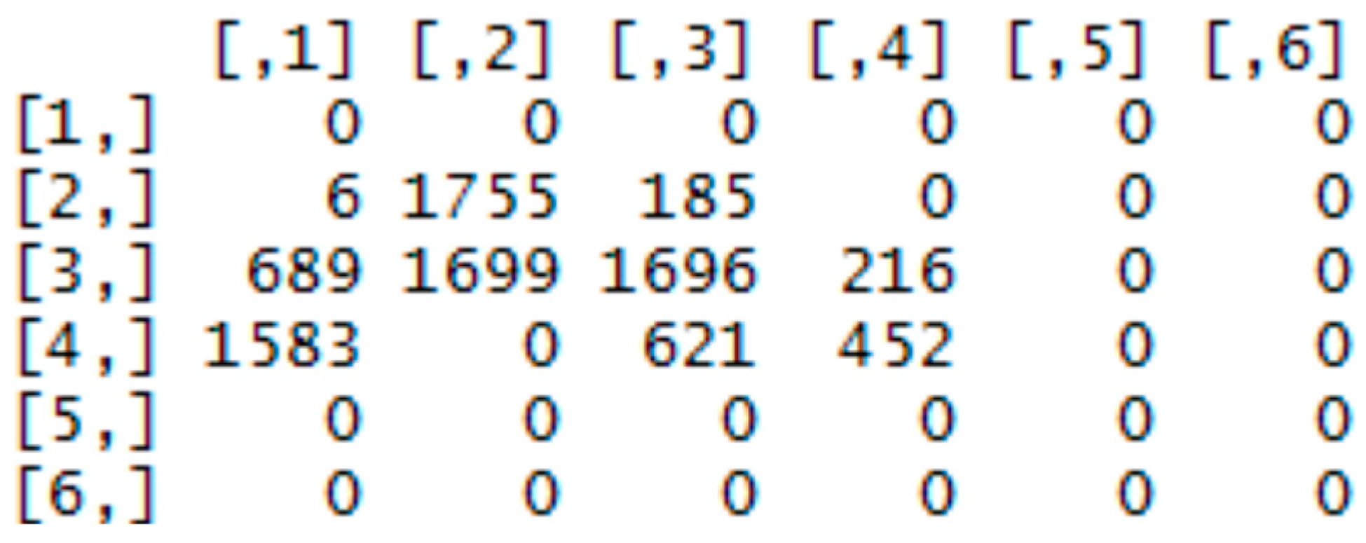
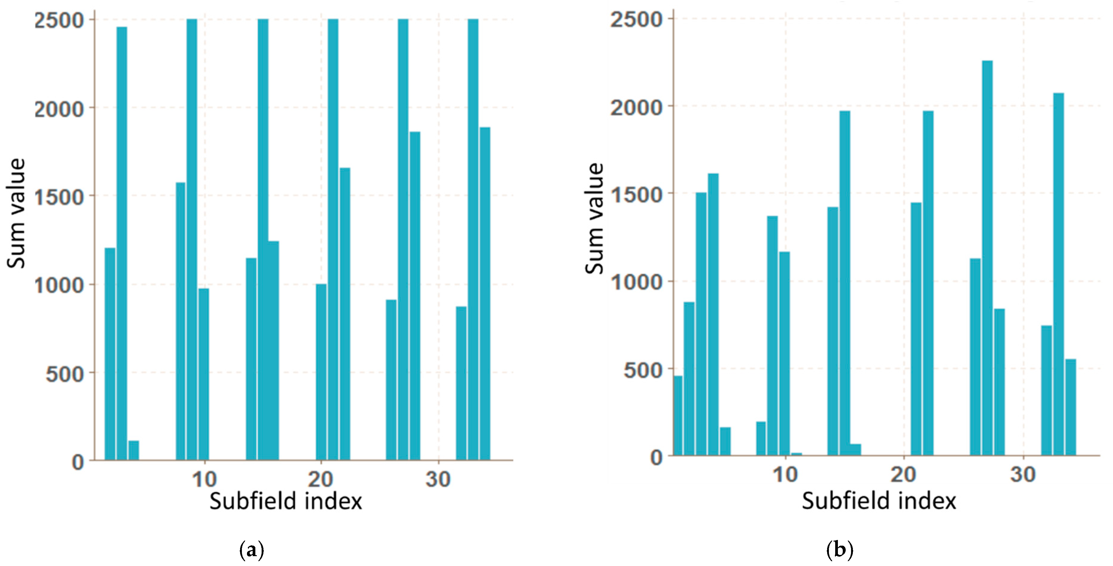
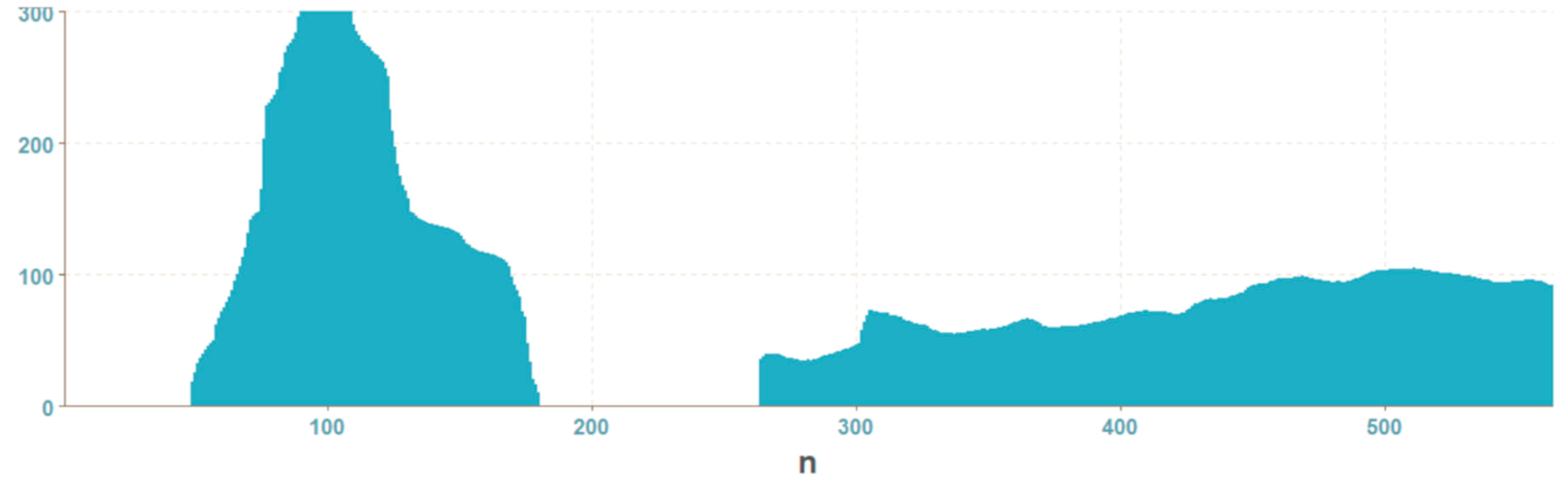
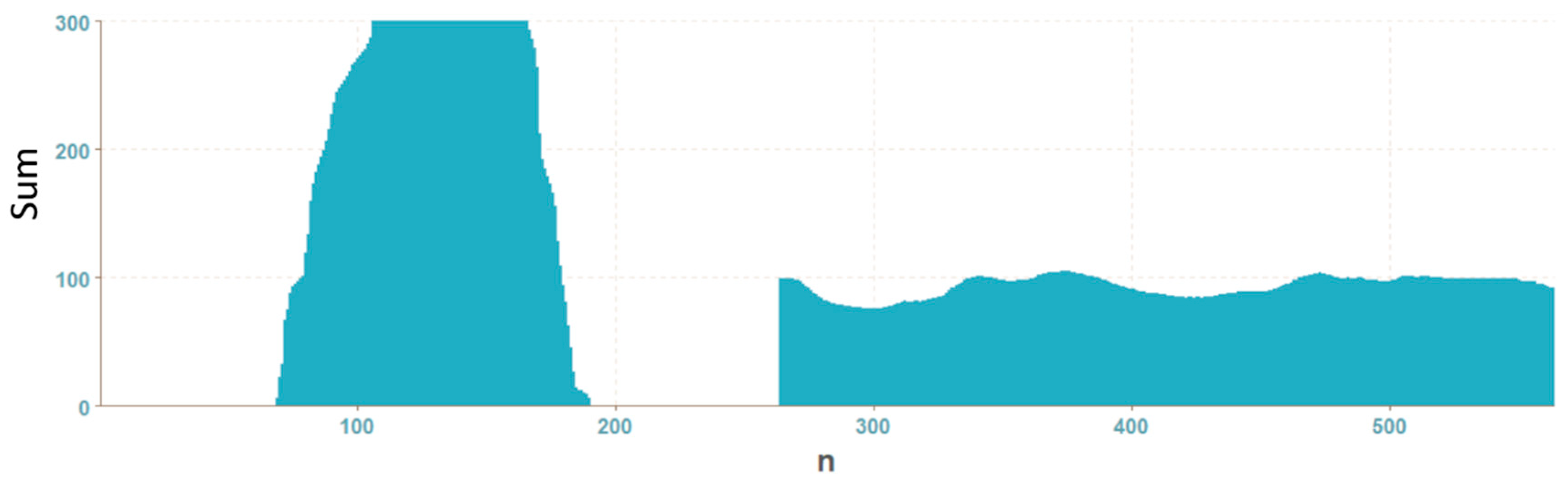
2.2. Vector of Sums of Subfields in the Mask
| Algorithm 1. Computing of subfields sums of the mask |
| procedure MaskToSums(img, size) xLen ←length(img[ ,1]) yLen ←length(img[1, ]) nRows ← ceiling(xLen/size) nCols ← ceiling(yLen/size) res ← matrix(0, nRows, nCols) for i in 1:xLen do for j in 1:yLen do if img[i,j] == TRUE then indI ← ceiling(i/size) indJ ← ceiling(j/size) res[indI, indJ] ++ end if end for end for return as.vector(res) end procedure |
2.3. Histogram Projection of the Mask
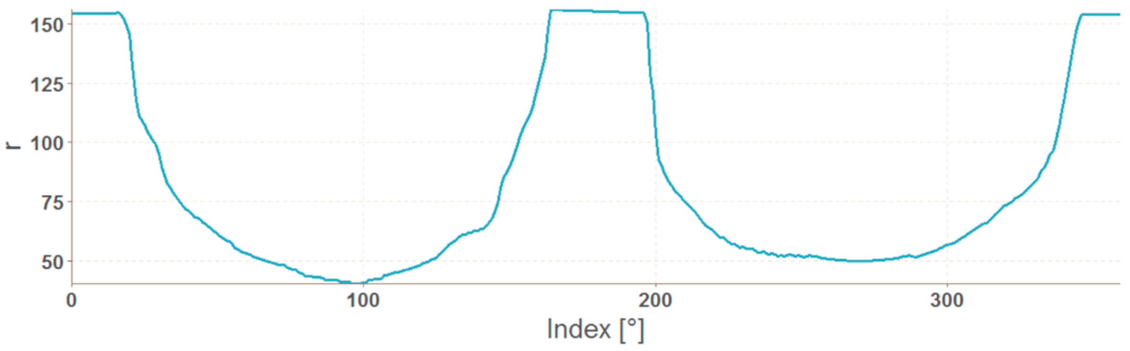
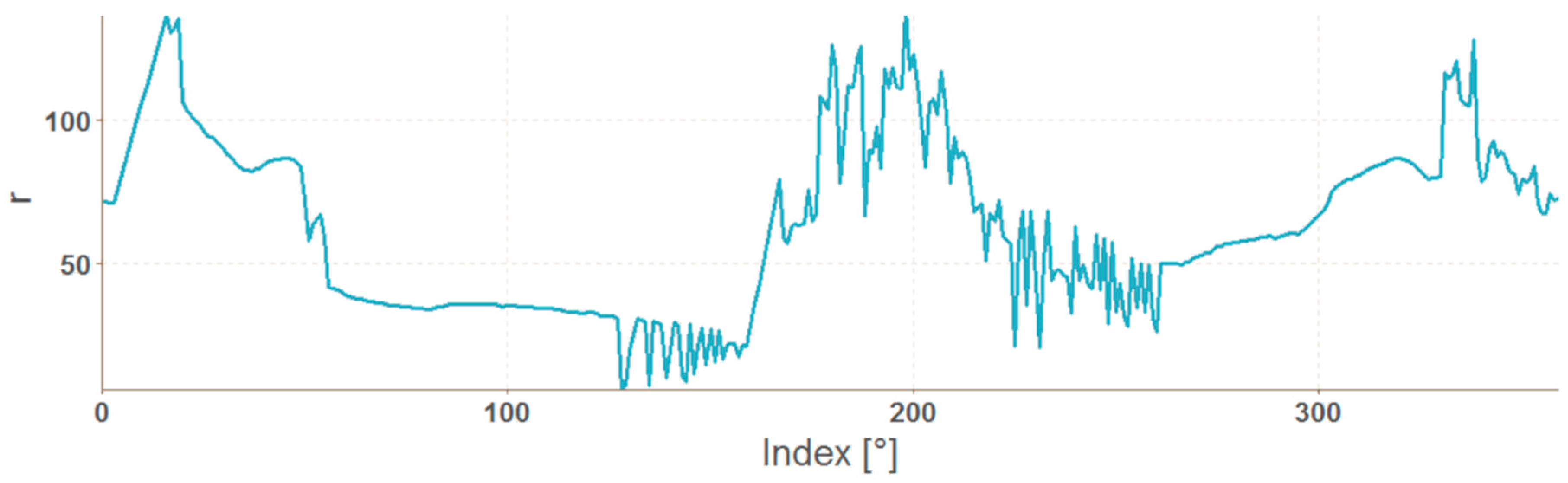
2.4. Vector of Polar Coordinates of the Mask Boundary
| Algorithm 2. Calculation of angle from Cartesian coordinates |
| procedure Angle(x, y) z ← x + 1i * y a ← 90 - arg(z) / π * 180 return round(a mod 360) end procedure |
2.5. Data Preparation for Neural Network
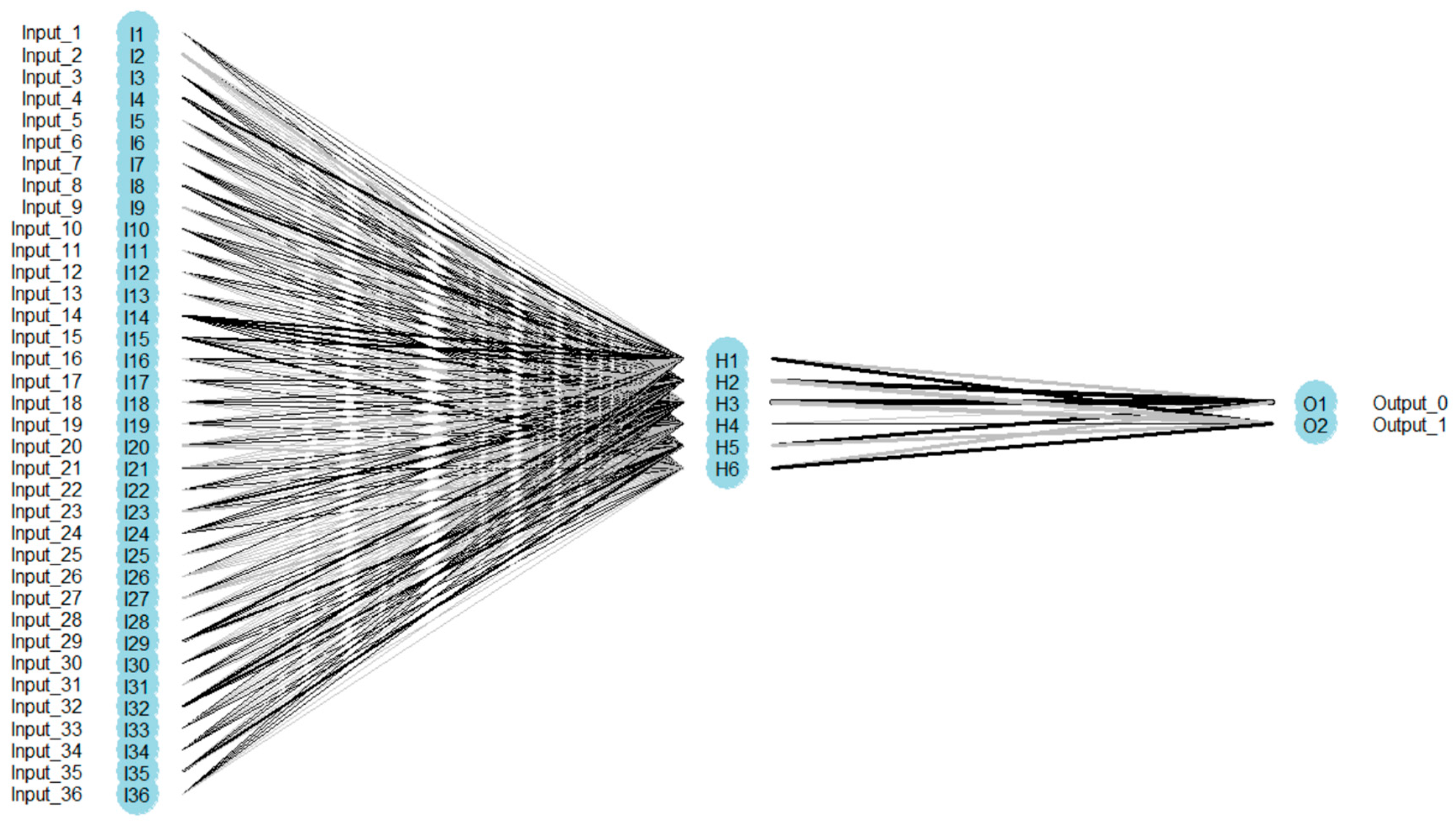
3. Configuration and Training of Neural Networks
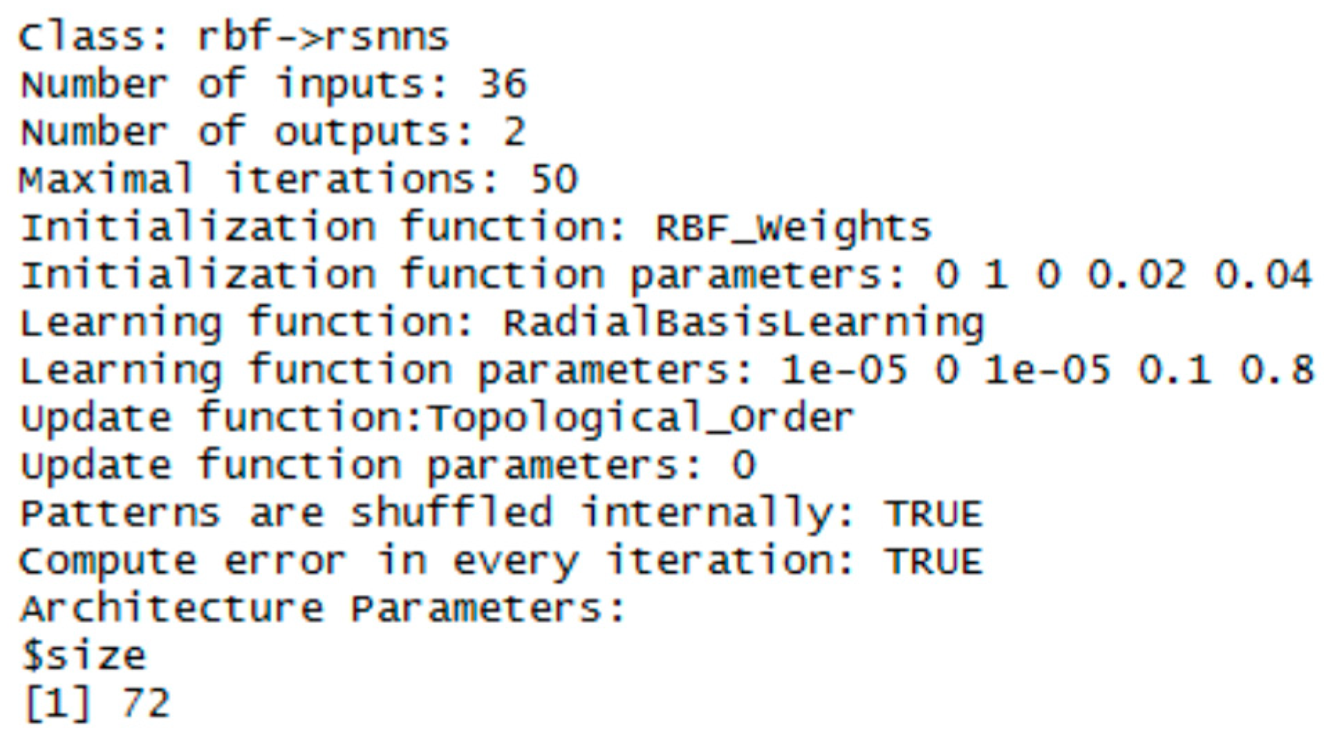
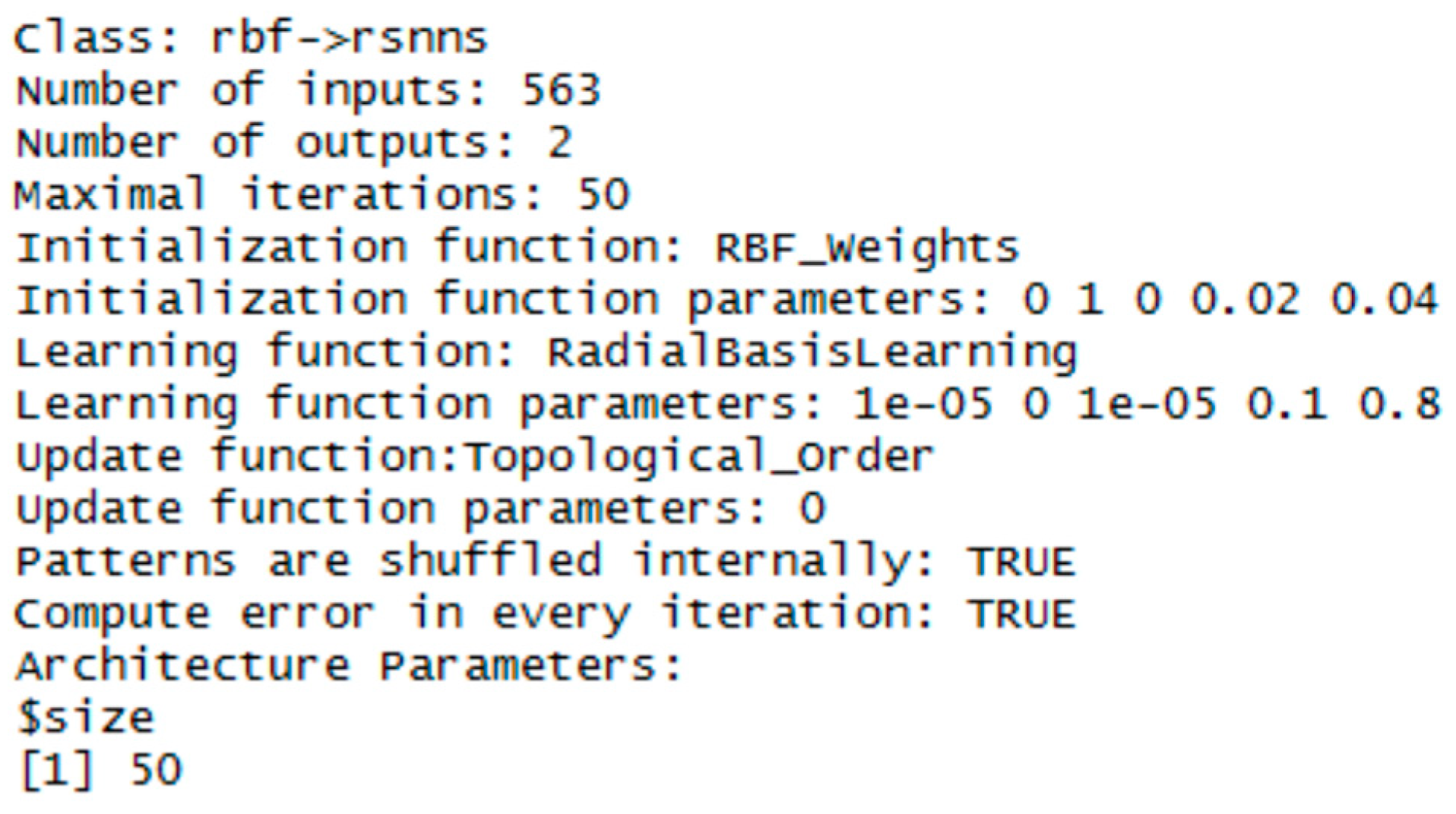
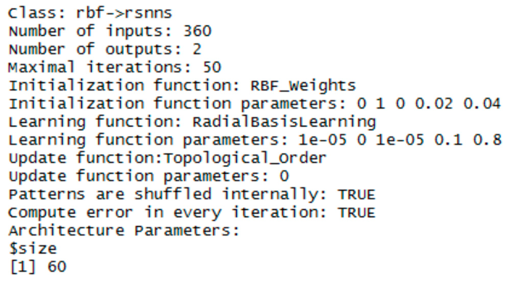
3.1. RBF Network
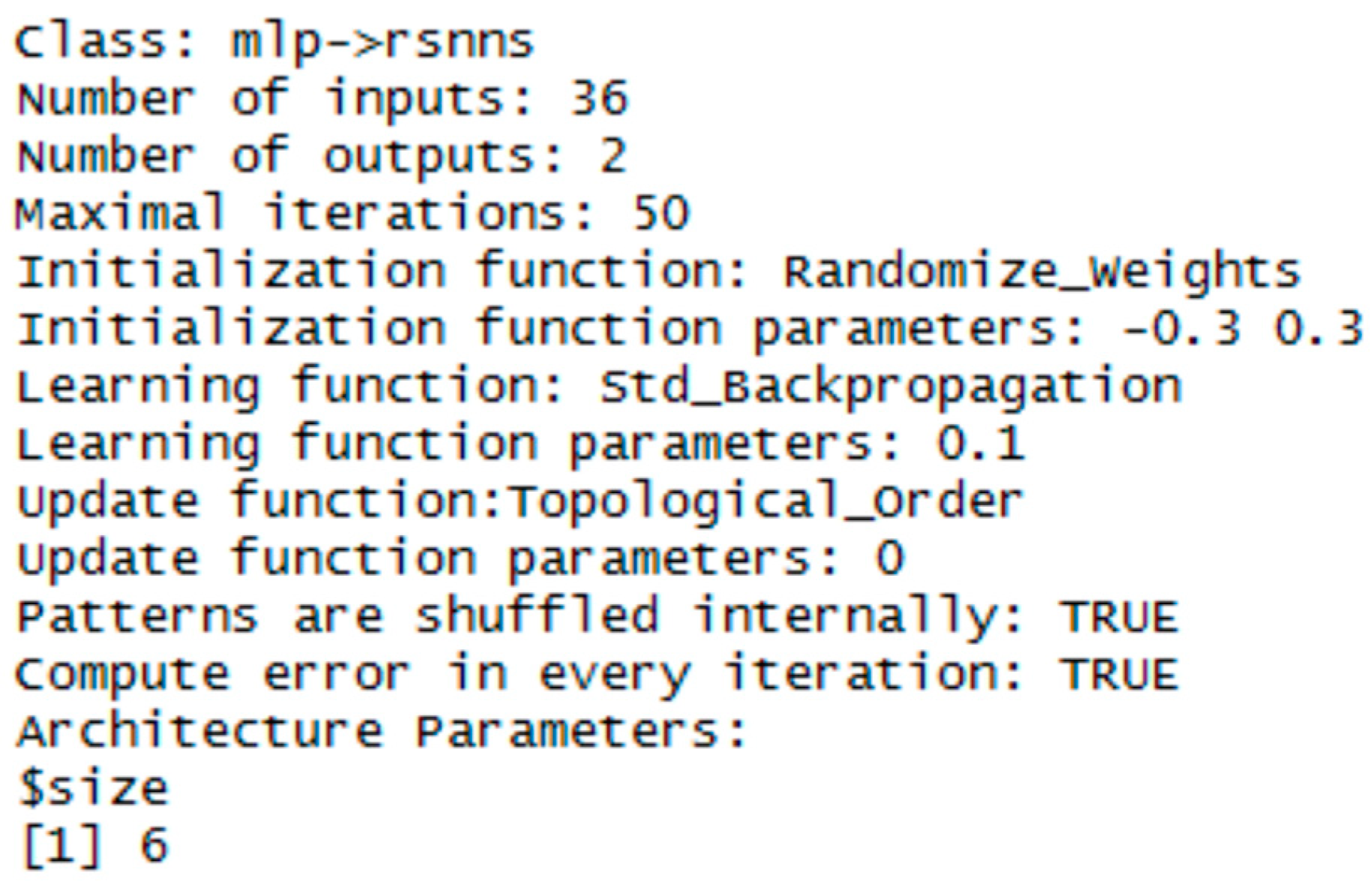
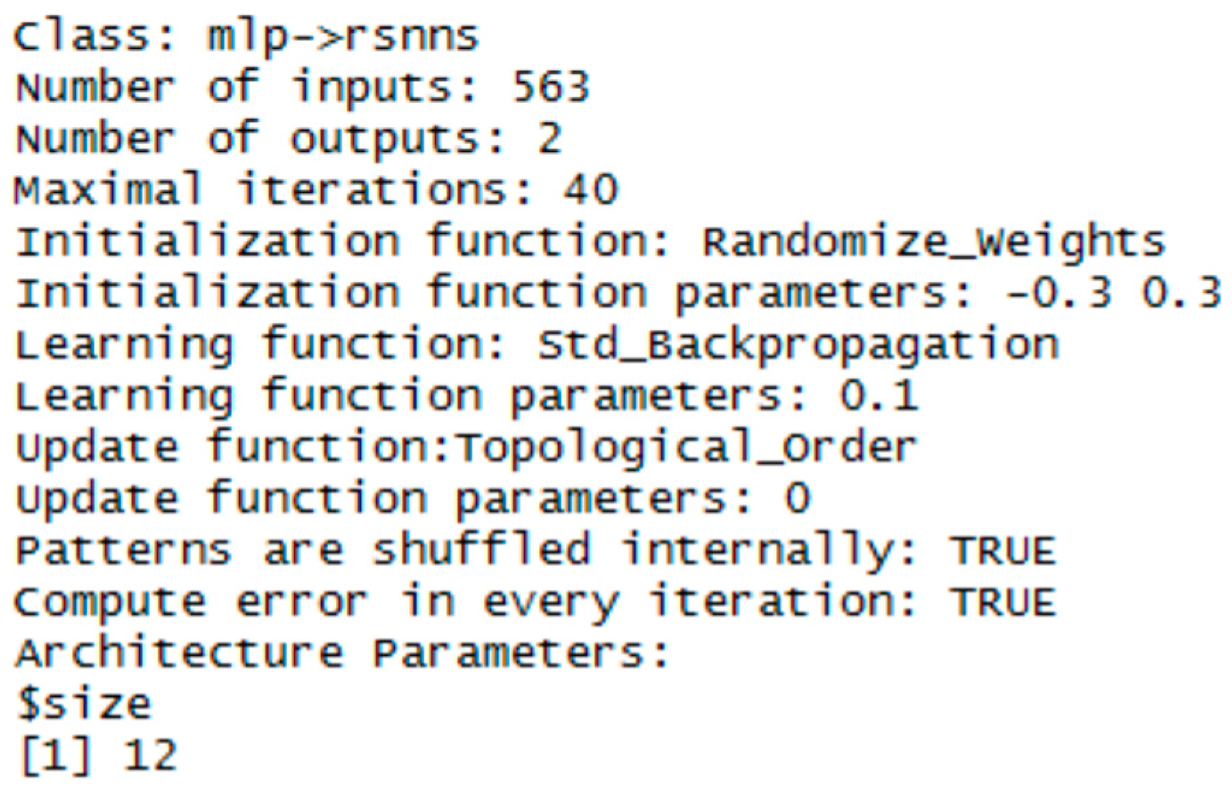
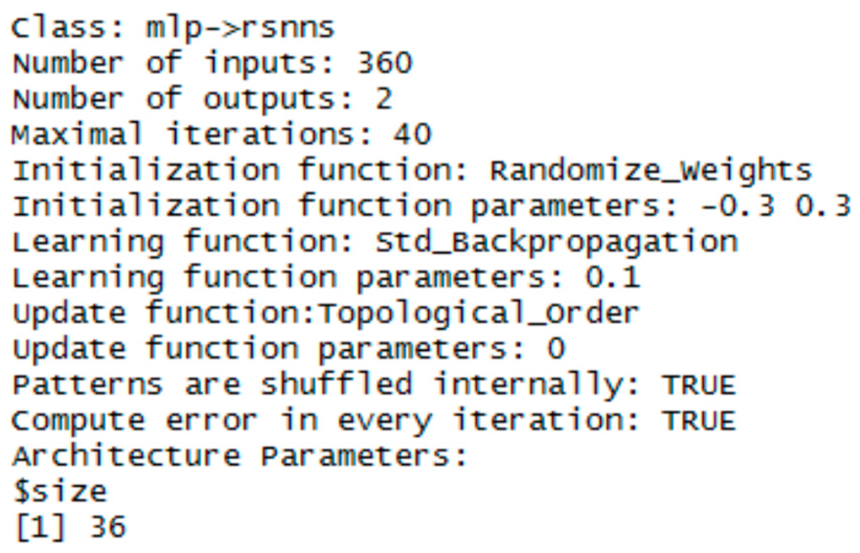
3.2. MLP Network
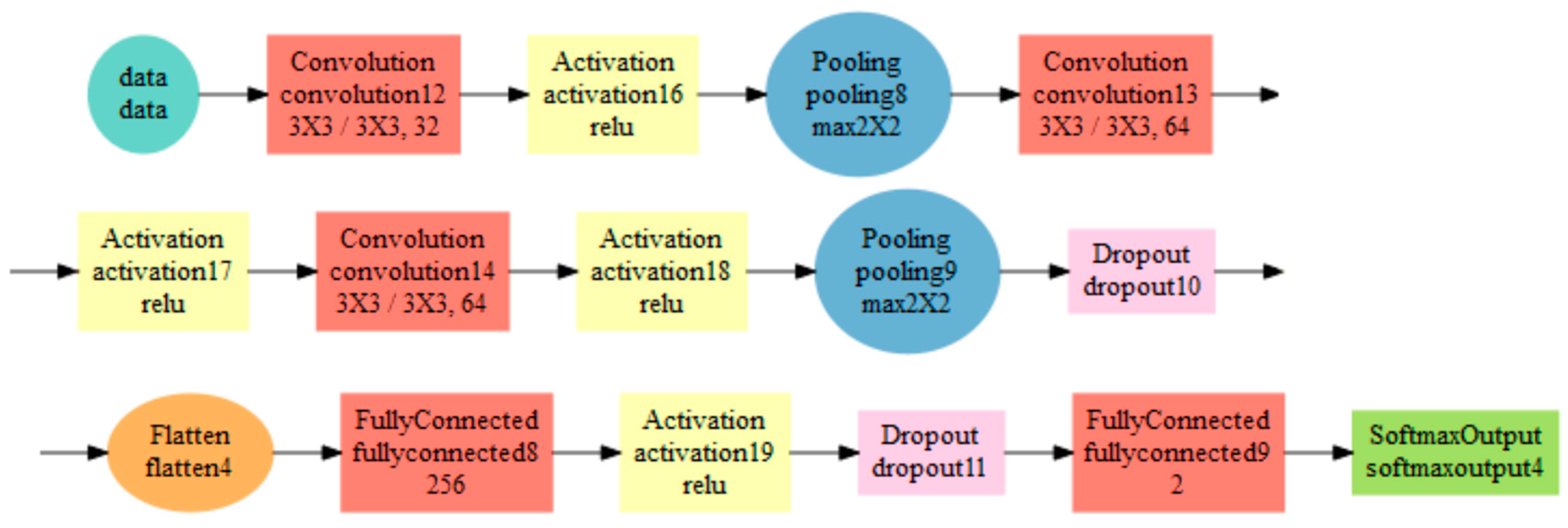
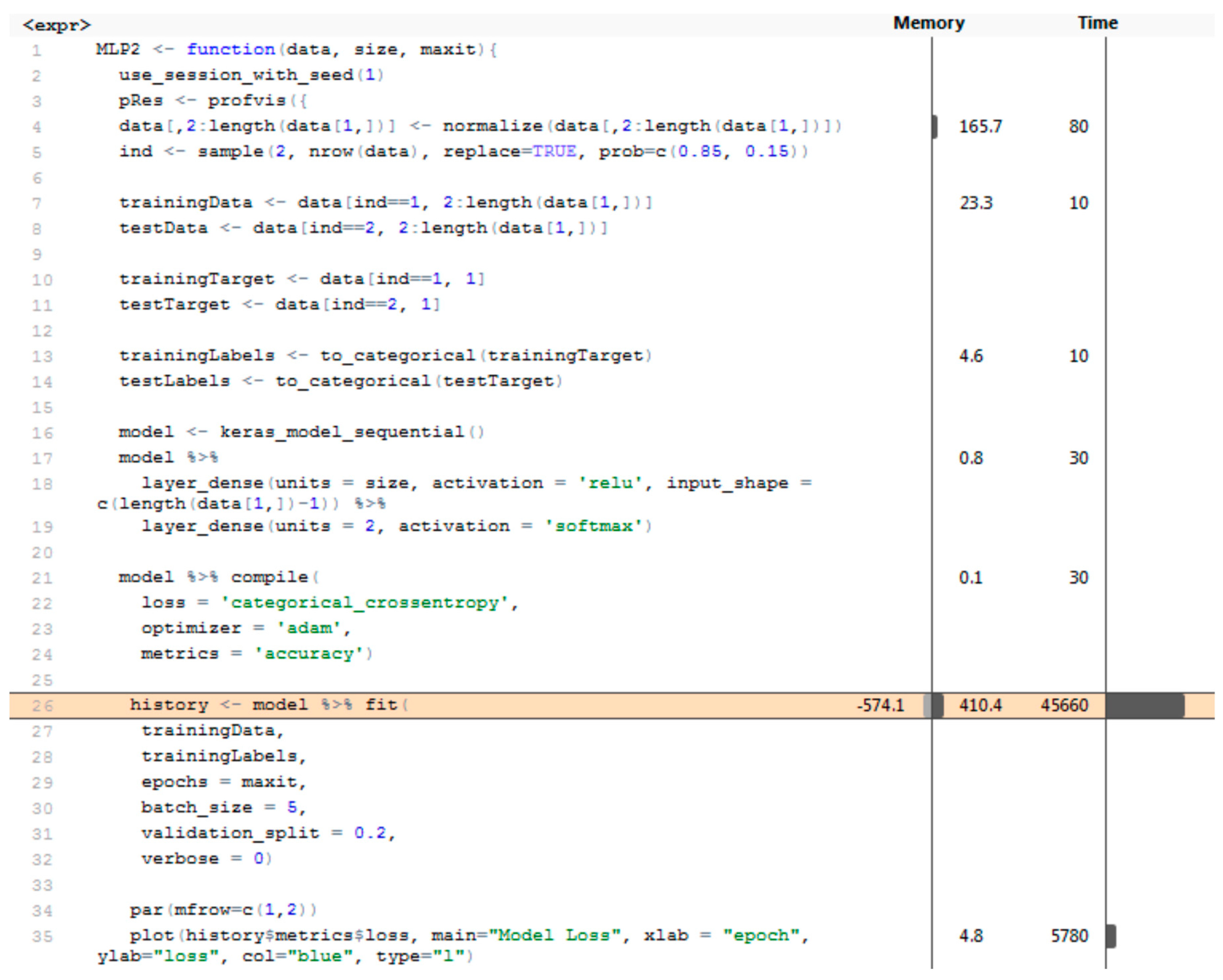
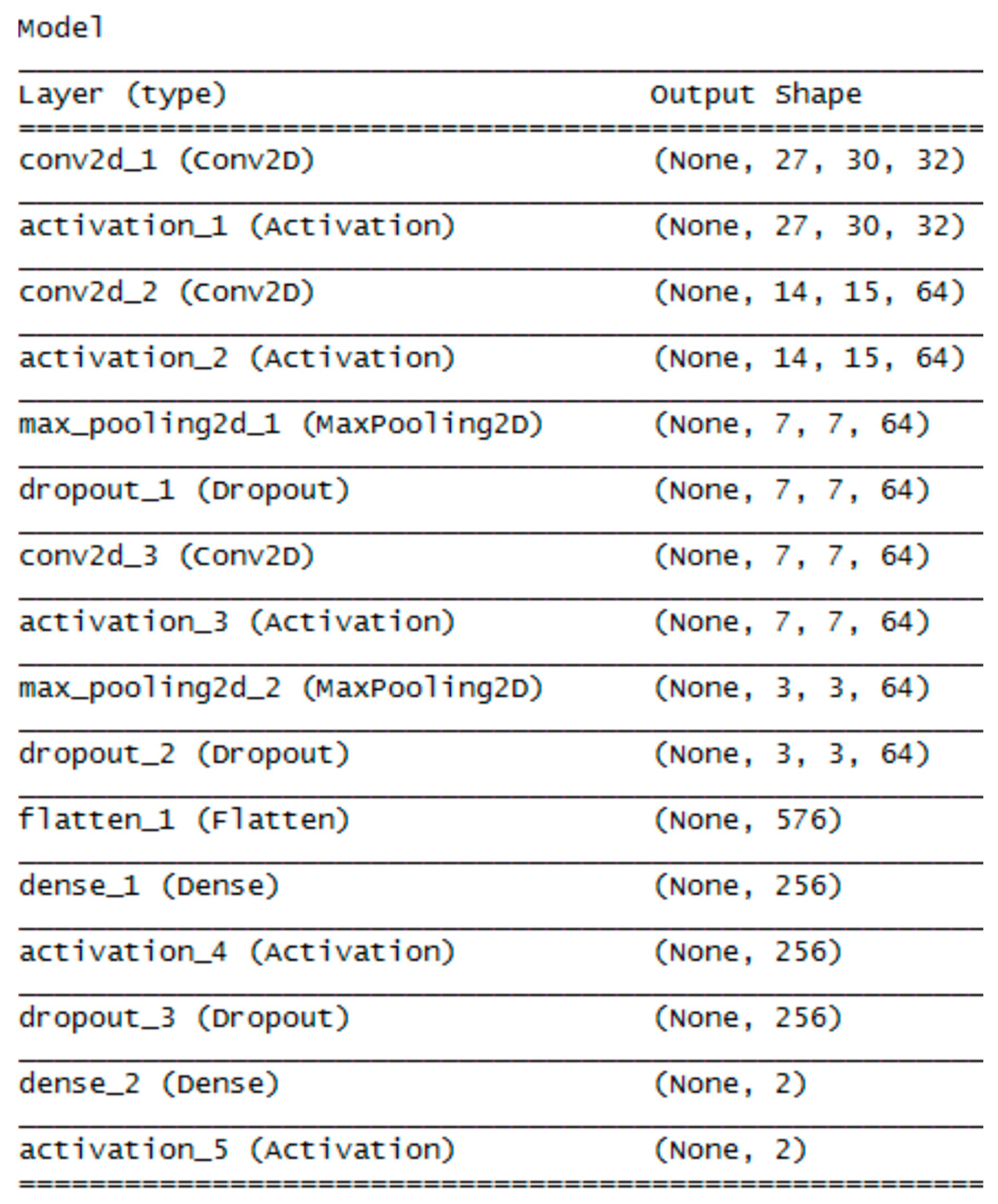
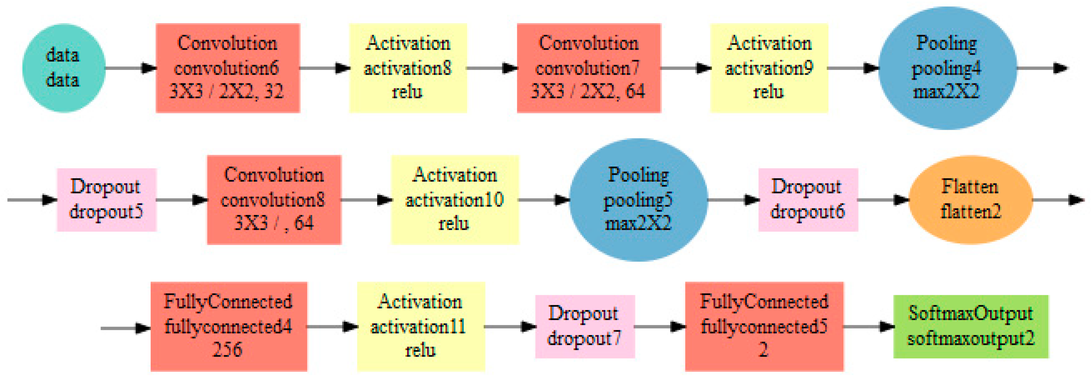
3.3. Convolution Neural Network
4. Results
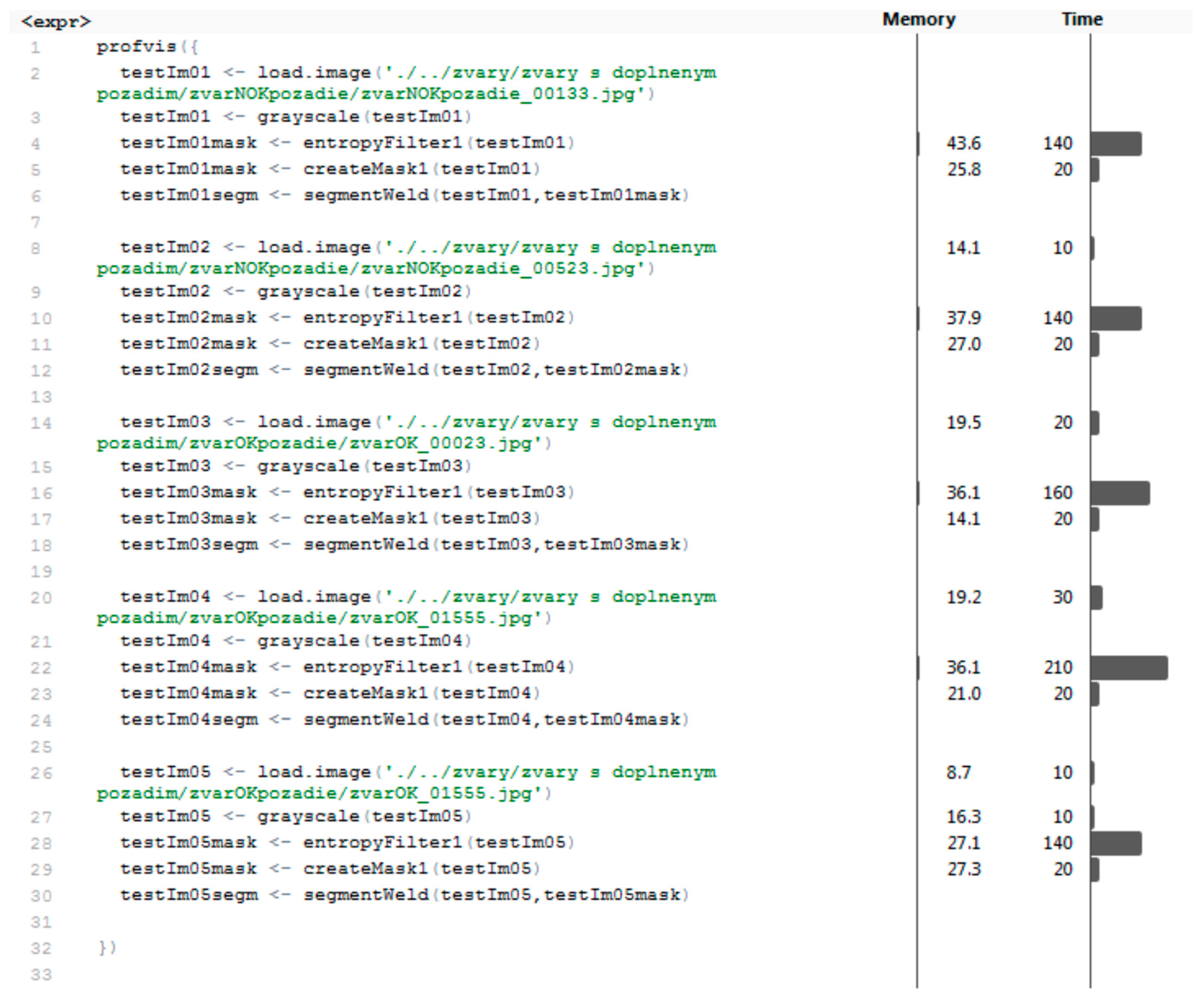
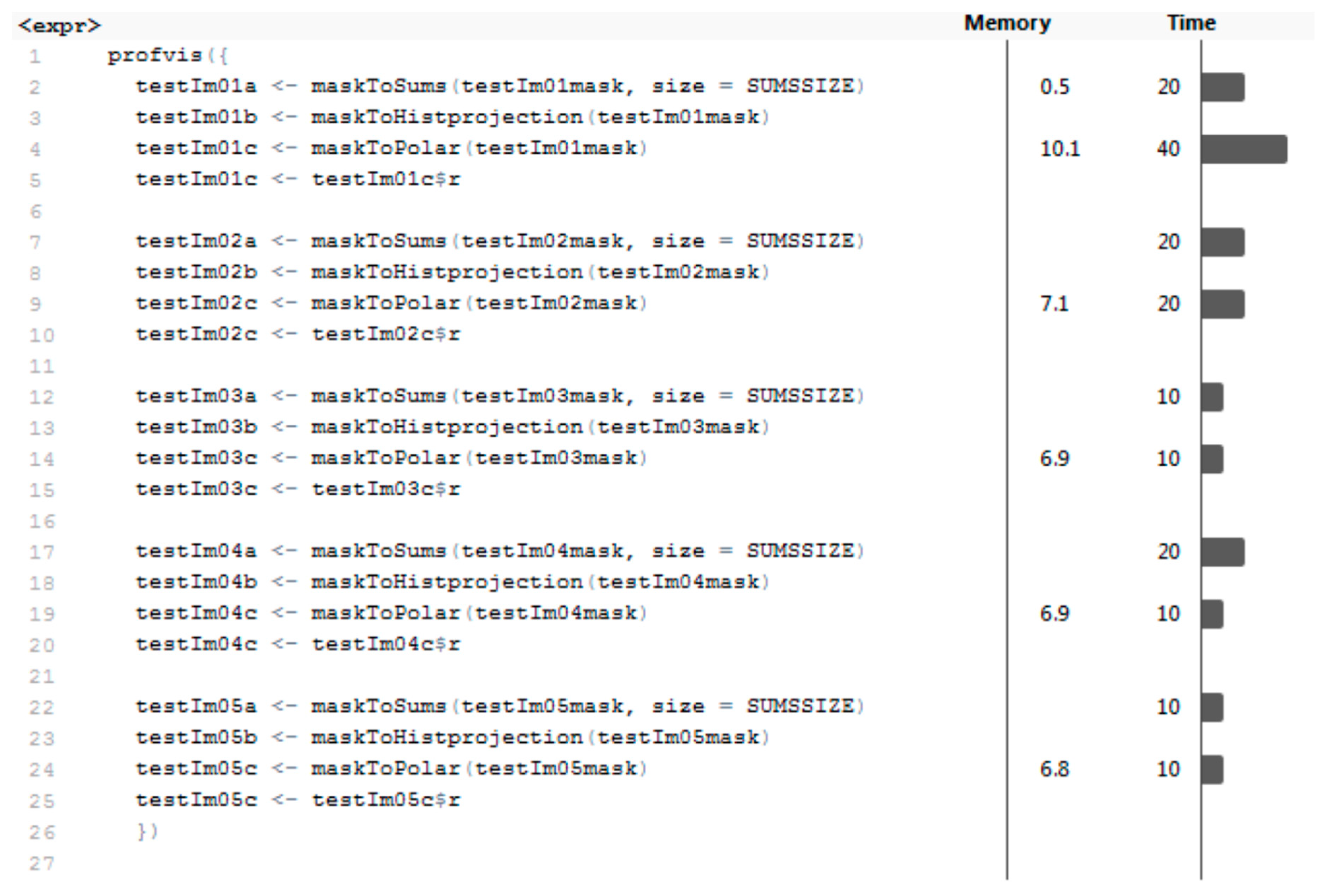
4.1. Code Profiling
4.2. Results of Data Preparation and Segmentation
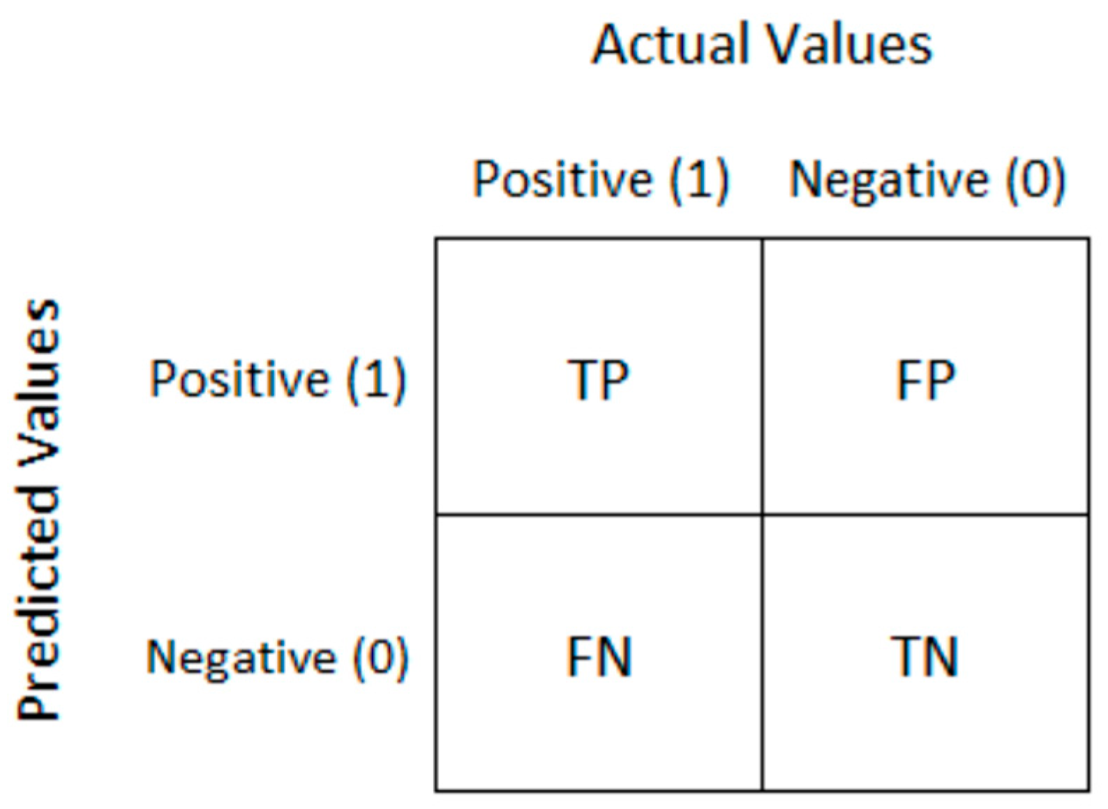
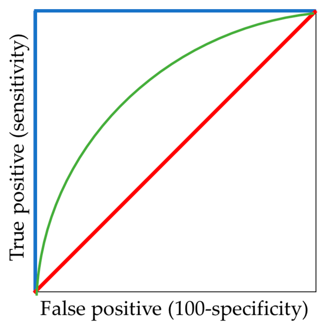
4.3. Criteria for Evaluation of Neural Network Results
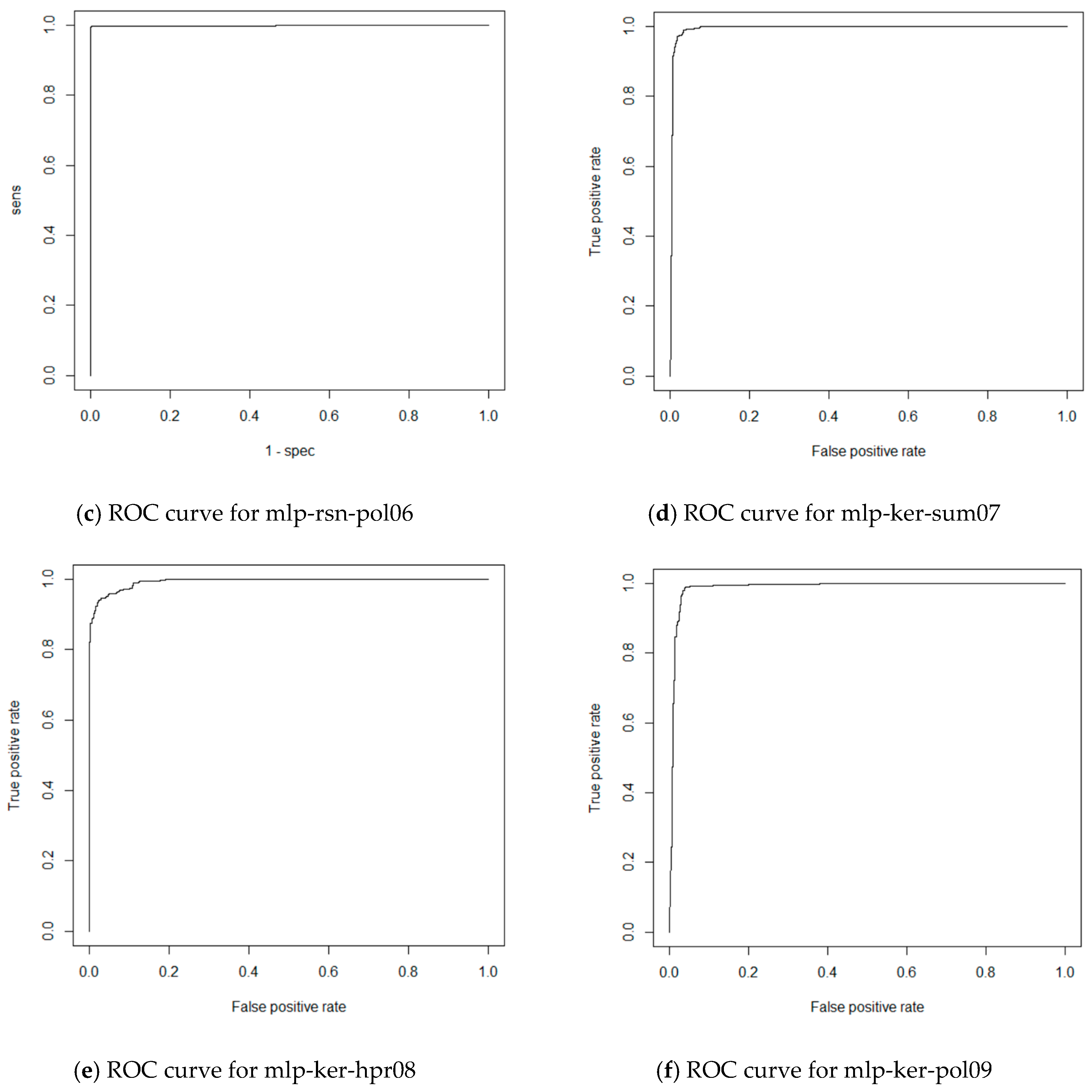
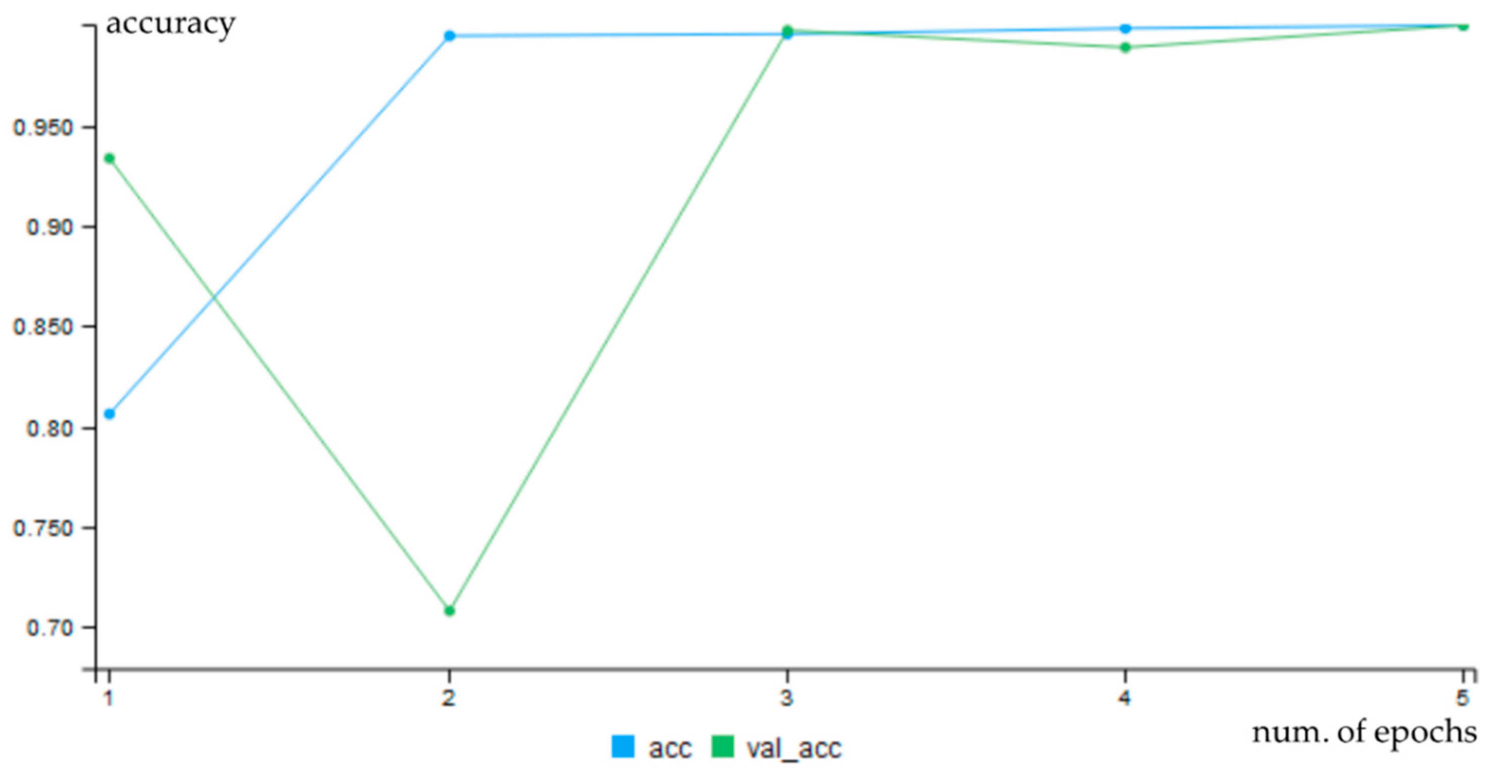
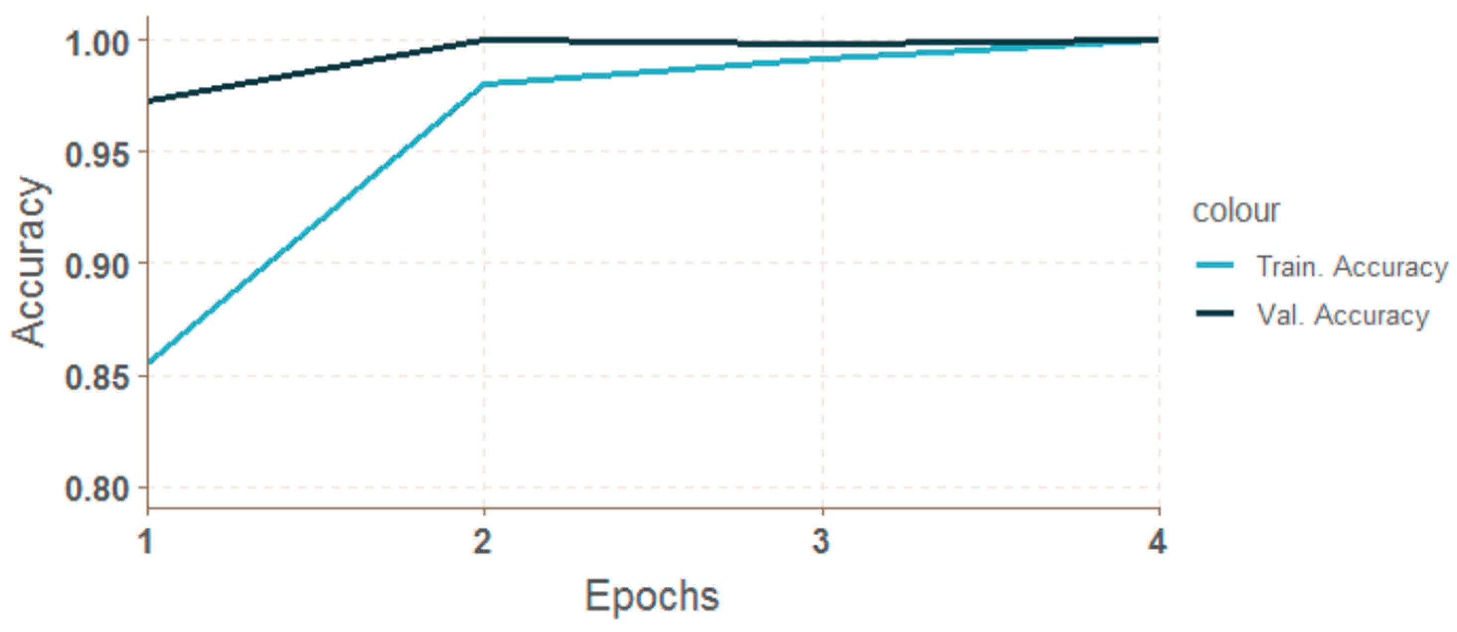
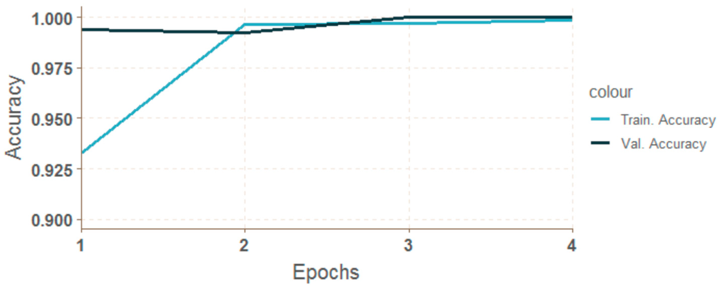
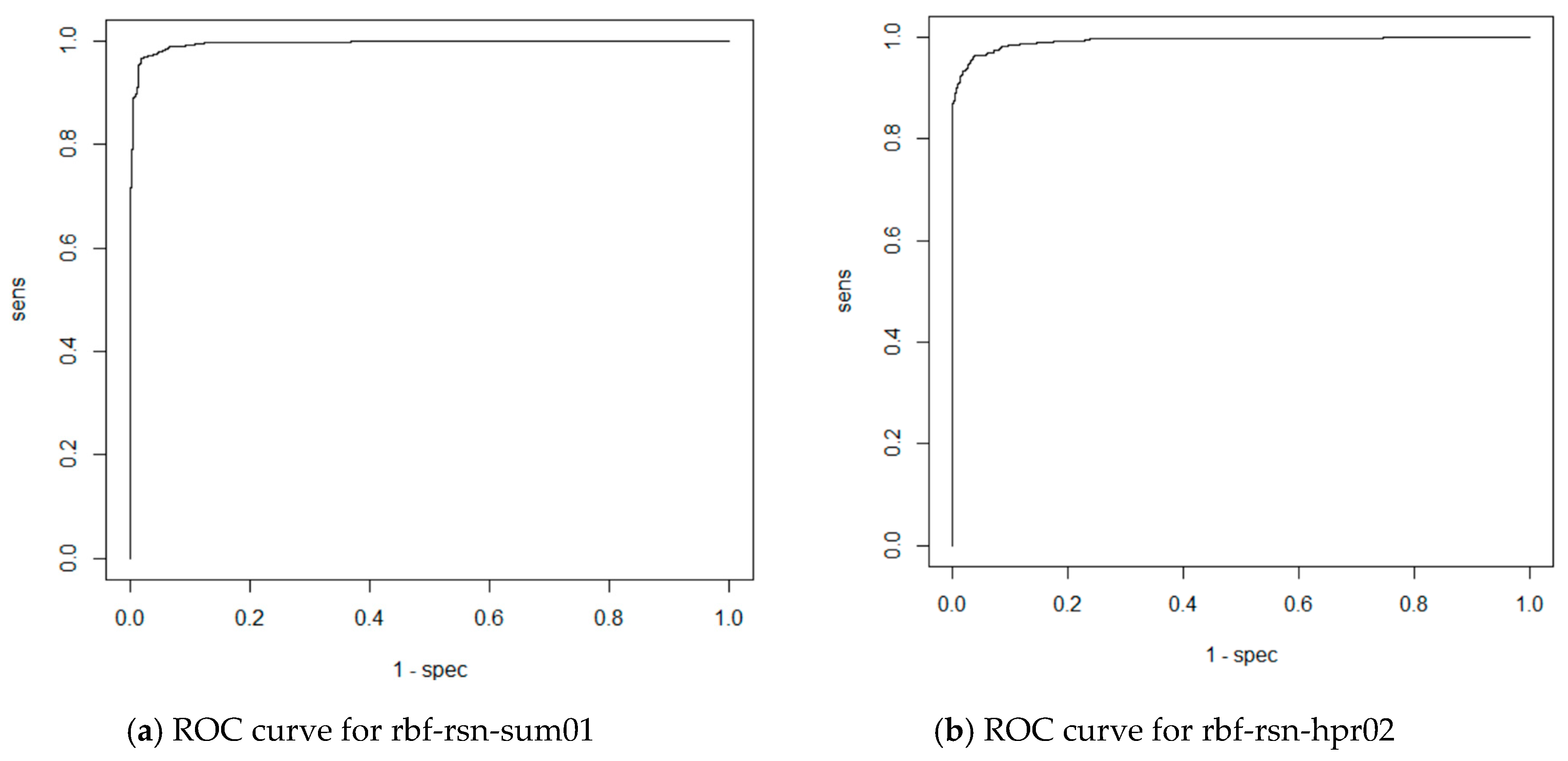
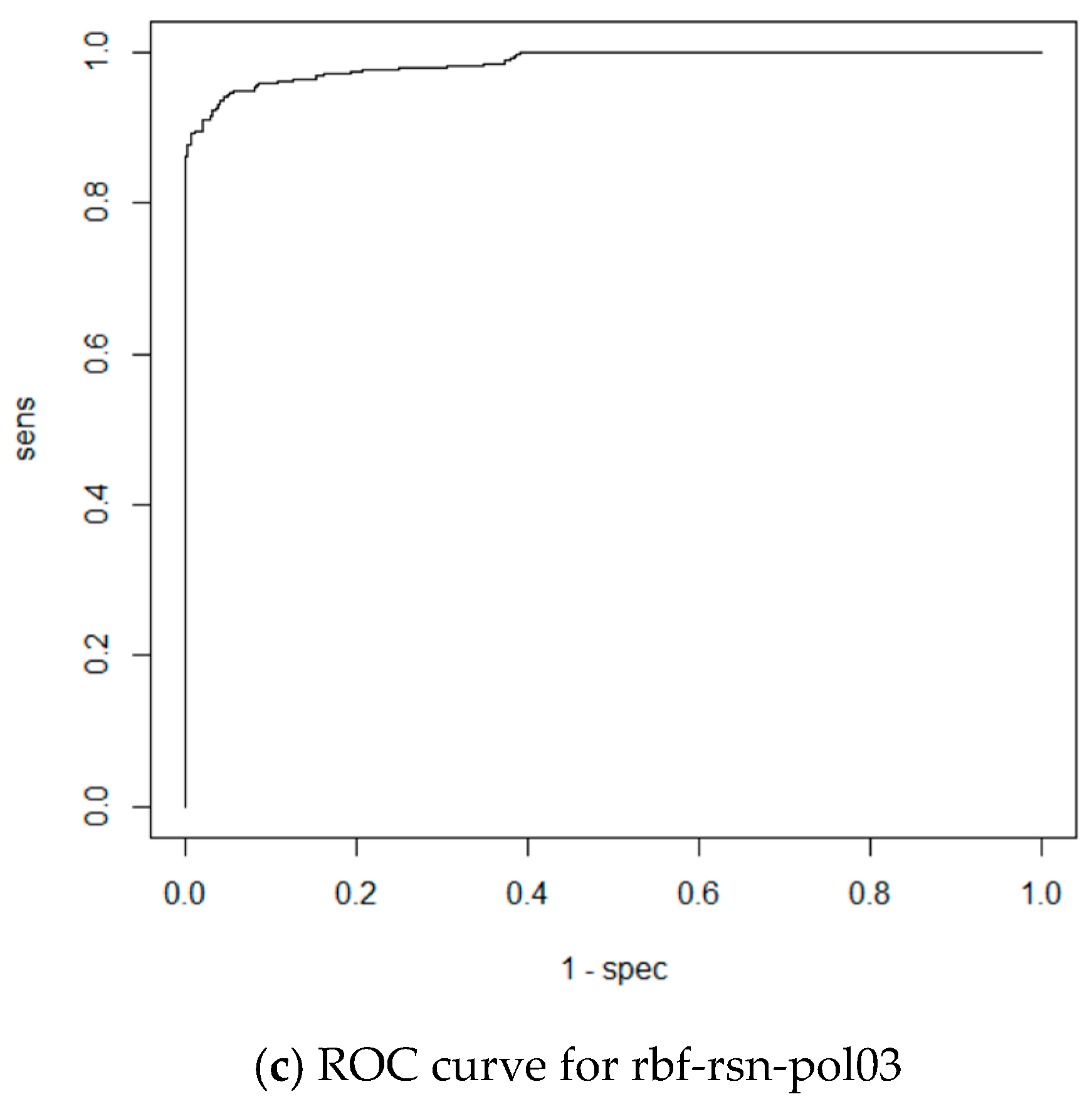
4.4. Results of Neural Network Classificaton
4.5. Profiling Single Weld Diagnostics
5. Discussion
Author Contributions
Funding
Acknowledgments
Conflicts of Interest
References
- Akşit, M. The Role of Computer Science and Software Technology in Organizing Universities for Industry 4.0 and beyond. In Proceedings of the 2018 Federated Conference on Computer Science and Information Systems, FedCSIS 2018, Poznań, Poland, 9–12 September 2018. [Google Scholar]
- Dahal, S.; Kim, T.; Ahn, K. Indirect prediction of welding fume diffusion inside a room using computational fluid dynamics. Atmosphere 2016, 7, 74. [Google Scholar] [CrossRef]
- Huang, W.; Kovacevic, R. A laser-based vision system for weld quality inspection. Sensors 2011, 11, 506–521. [Google Scholar] [CrossRef] [PubMed]
- Noruk, J. Visual weld inspection enters the new millennium. Sens. Rev. 2001, 21, 278–282. [Google Scholar] [CrossRef]
- Deng, S.; Jiang, L.; Jiao, X.; Xue, L.; Deng, X. Image processing of weld seam based on beamlet transform. Hanjie Xuebao/Trans. China Weld. Inst. 2009, 30, 68–72. [Google Scholar]
- Deng, S.; Jiang, L.; Jiao, X.; Xue, L.; Cao, Y. Weld seam edge extraction algorithm based on Beamlet Transform. In Proceedings of the 1st International Congress on Image and Signal Processing, CISP 2008, Hainan, China, 27–30 May 2008. [Google Scholar]
- Zhang, X.; Yin, Z.; Xiong, Y. Edge detection of the low contrast welded joint image corrupted by noise. In Proceedings of the 8th International Conference on Electronic Measurement and Instruments, ICEMI 2007, Xi’an, China, 16–18 August 2007. [Google Scholar]
- Hou, X.; Liu, H. Welding image edge detection and identification research based on canny operator. In Proceedings of the 2012 International Conference on Computer Science and Service Systems, CSSS 2012, Nanjing, China, 11–13 August 2012. [Google Scholar]
- Shen, Z.; Sun, J. Welding seam defect detection for canisters based on computer vision. In Proceedings of the 6th International Congress on Image and Signal Processing, CISP 2013, Hangzhou, China, 16–18 December 2013. [Google Scholar]
- Liao, Z.; Sun, J. Image segmentation in weld defect detection based on modified background subtraction. In Proceedings of the 6th International Congress on Image and Signal Processing, CISP 2013, Hangzhou, China, 16–18 December 2013. [Google Scholar]
- Khumaidi, A.; Yuniarno, E.M.; Purnomo, M.H. Welding defect classification based on convolution neural network (CNN) and Gaussian Kernel. In Proceedings of the 2017 International Seminar on Intelligent Technology and Its Application: Strengthening the Link between University Research and Industry to Support ASEAN Energy Sector, ISITIA 2017, Surabaya, Indonesia, 28–29 August 2017. [Google Scholar]
- Pandiyan, V.; Murugan, P.; Tjahjowidodo, T.; Caesarendra, W.; Manyar, O.M.; Then, D.J.H. In-process virtual verification of weld seam removal in robotic abrasive belt grinding process using deep learning. Robot. Comput. Integr. Manuf. 2019, 57, 477–487. [Google Scholar] [CrossRef]
- Chen, J.; Wang, T.; Gao, X.; Wei, L. Real-time monitoring of high-power disk laser welding based on support vector machine. Comput. Ind. 2018, 94, 75–81. [Google Scholar] [CrossRef]
- Wang, T.; Chen, J.; Gao, X.; Qin, Y. Real-time monitoring for disk laser welding based on feature selection and SVM. Appl. Sci. 2017, 7, 884. [Google Scholar] [CrossRef]
- Haffner, O.; Kucera, E.; Kozak, S.; Stark, E. Proposal of system for automatic weld evaluation. In Proceedings of the 21st International Conference on Process Control, PC 2017, Štrbské Pleso, Slovakia, 6–9 June 2017. [Google Scholar]
- Haffner, O.; Kučera, E.; Kozák, Š. Weld segmentation for diagnostic and evaluation method. In Proceedings of the 2016 Cybernetics and Informatics, K and I 2016—Proceedings of the the 28th International Conference, Levoca, Slovakia, 2–5 February 2016. [Google Scholar]
- Haffner, O.; Kučera, E.; Kozák, Š.; Stark, E. Application of Pattern Recognition for a Welding Process. In Proceedings of the Communiation Papers of the 2017 Federated Conference on Computer Science and Information Systems, FedCSIS 2017, Prague, Czech Republic, 3–6 September 2017. [Google Scholar]
- Haffner, O.; Kučera, E.; Bachurikova, M. Proposal of weld inspection system with single-board computer and Android smartphone. In Proceedings of the 2016 Cybernetics and Informatics, K and I 2016—Proceedings of the the 28th International Conference, Levoca, Slovakia, 2–5 February 2016. [Google Scholar]
- Gajowniczek, K.; Ząbkowski, T.; Orłowski, A. Comparison of decision trees with Rényi and Tsallis entropy applied for imbalanced churn dataset. In Proceedings of the 2015 Federated Conference on Computer Science and Information Systems, FedCSIS 2015, Łódź, Poland, 13–16 September 2015. [Google Scholar]
- Sokolova, M.; Lapalme, G. A systematic analysis of performance measures for classification tasks. Inf. Process. Manag. 2009, 45, 427–437. [Google Scholar] [CrossRef]


| Operating System | Windows 7 Professional 64-bit |
| Processor | Intel Core i7-2600 CPU @ 3,40 GHz |
| Memory | 16 GB DDR3 |
| Disc | Samsung SSD 850 EVO 500 GB |
| Data Interpretation | Time [ms] | Memory [MB] |
|---|---|---|
| the vector of sums of subfields in the mask | 16 | 0.1 |
| histogram projection vector | 10 | 0.1 |
| polar coordinates vector | 18 | 7.56 |
| Test Label | Network Type | Library | Data Format |
|---|---|---|---|
| rbf-rsn-sum01 | RBF | RSNNS | Subfields sum |
| rbf-rsn-hpr02 | RBF | RSNNS | Histogram projection |
| rbf-rsn-pol03 | RBF | RSNNS | Polar coordinates |
| mlp-rsn-sum04 | MLP | RSNNS | Subfields sum |
| mlp-rsn-hpr05 | MLP | RSNNS | Histogram projection |
| mlp-rsn-pol06 | MLP | RSNNS | Polar coordinates |
| mlp-ker-sum07 | MLP | Keras | Subfields sum |
| mlp-ker-hpr08 | MLP | Keras | Histogram projection |
| mlp-ker-pol09 | MLP | Keras | Polar coordinates |
| cnn-ker-ori10 | CNN 1 | Keras | Original |
| cnn-ker-seg11 | CNN 1 | Keras | Segmented |
| cnn-mxn-ori12 | CNN 1 | MXNet | Original |
| cnn-mxn-seg13 | CNN 1 | MXNet | Segmented |
| cnn-mxn-ori14 | CNN 2 | MXNet | Original |
| cnn-mxn-seg15 | CNN 2 | MXNet | Segmented |
| Test Label | Accuracy | F-Score |
|---|---|---|
| rbf-rsn-sum01 | 0.9699 | 0.9719 |
| rbf-rsn-hpr02 | 0.9139 | 0.9127 |
| rbf-rsn-pol03 | 0.9149 | 0.9139 |
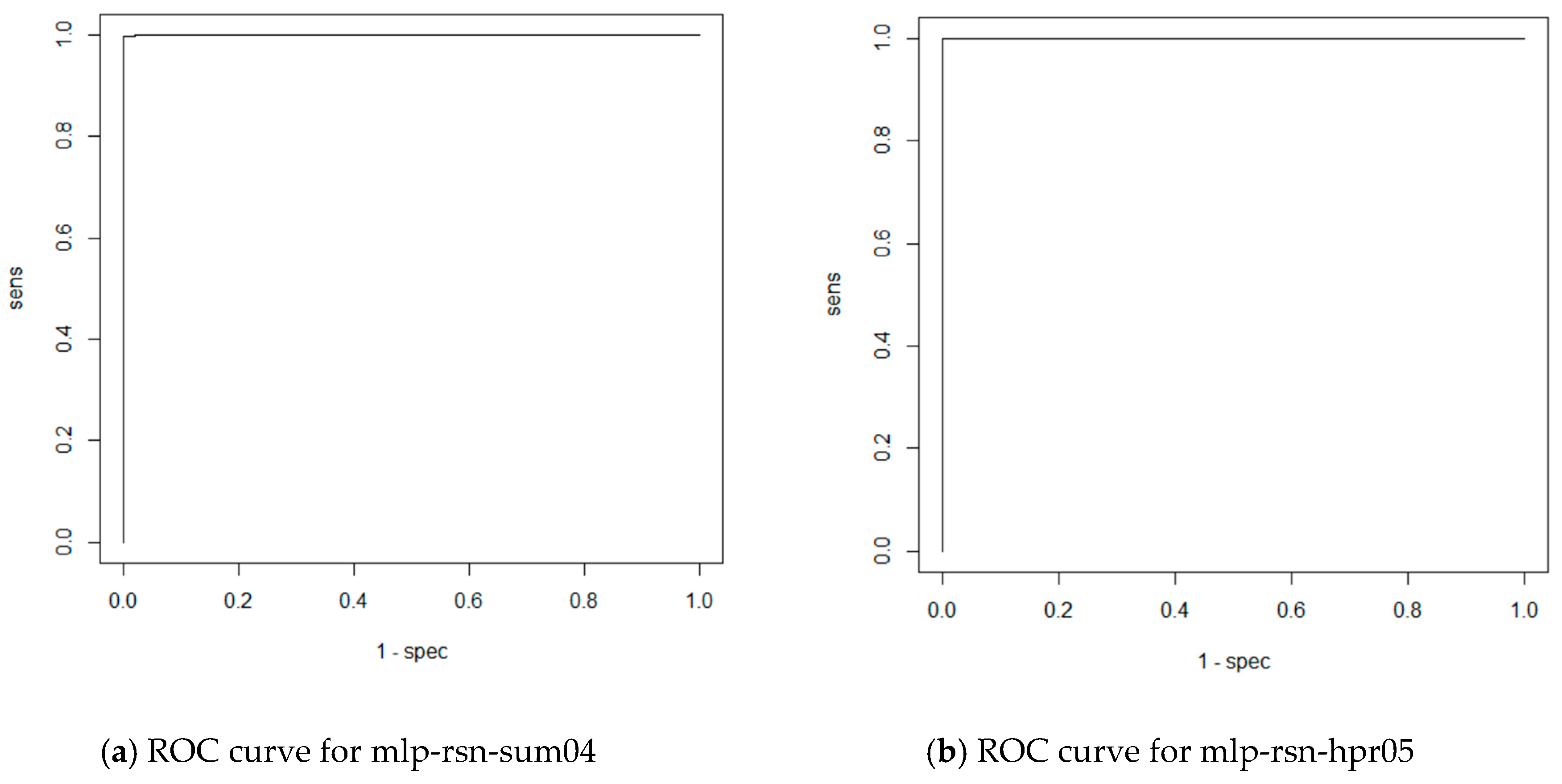
| mlp-rsn-sum04 | 0.9979 | 0.9981 |
| mlp-rsn-hpr05 | 1.0000 | 1.0000 |
| mlp-rsn-pol06 | 0.9959 | 0.9961 |
| mlp-ker-sum07 | 0.9678 | 0.9700 |
| mlp-ker-hpr08 | 0.9761 | 0.9761 |
| mlp-ker-pol09 | 0.9766 | 0.9766 |
| Test Label. | Time [ms] | Memory [MB] |
|---|---|---|
| rbf-rsn-sum01 | 6660 | 687.6 |
| rbf-rsn-hpr02 | 42,530 | 775.6 |
| rbf-rsn-pol03 | 32,080 | 752.3 |
| mlp-rsn-sum04 | 850 | 769.8 |
| mlp-rsn-hpr05 | 9890 | 653.7 |
| mlp-rsn-pol06 | 17,270 | 672.0 |
| mlp-ker-sum07 | 52,830 | 485.2 |
| mlp-ker-hpr08 | 45,660 | 410.4 |
| mlp-ker-pol09 | 46,420 | 401.9 |
| Test Label | Epochs | Accuracy | F-Score |
|---|---|---|---|
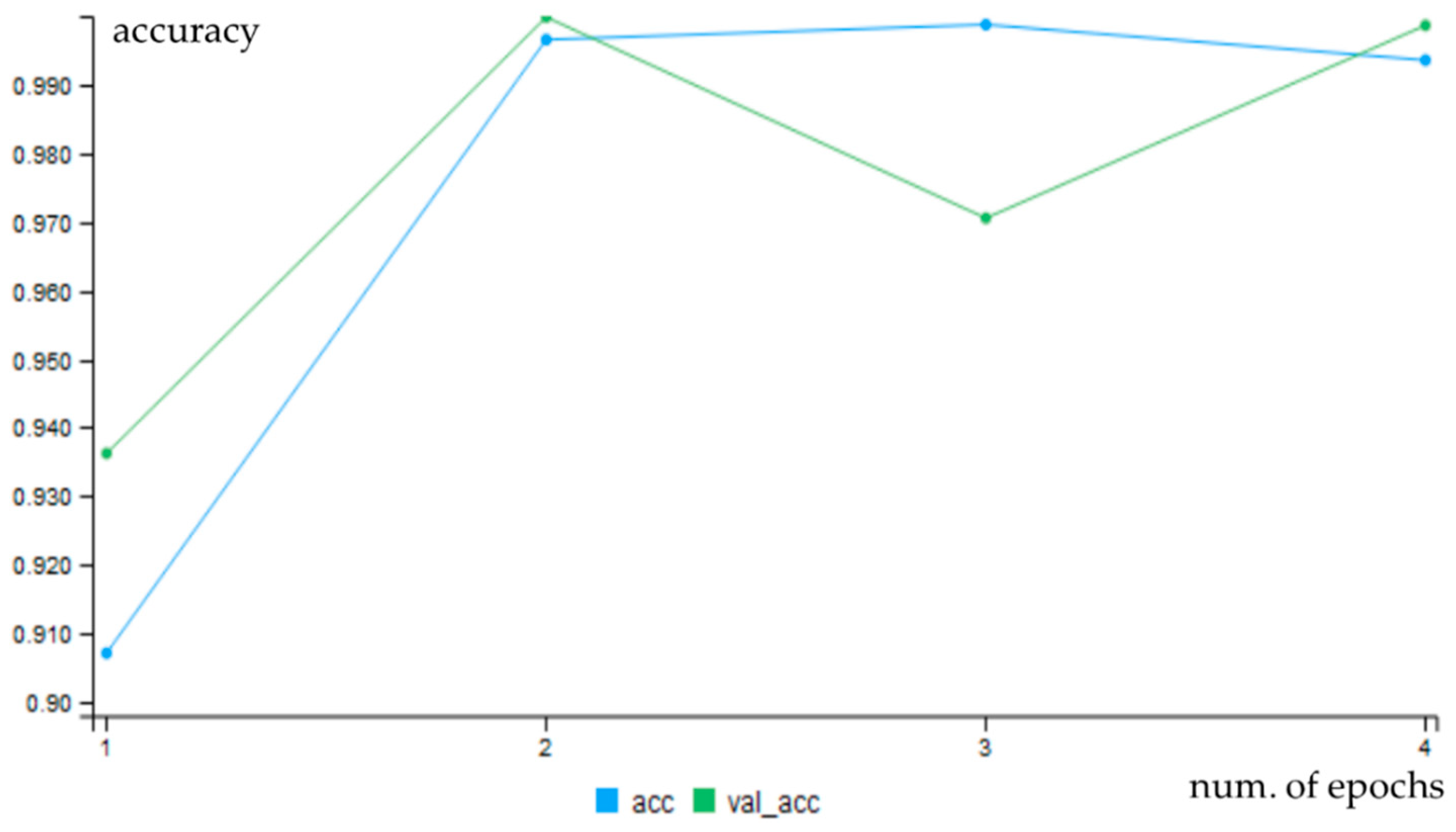
| cnn-ker-ori10 | 5 | 0.9990 | 0.9991 |
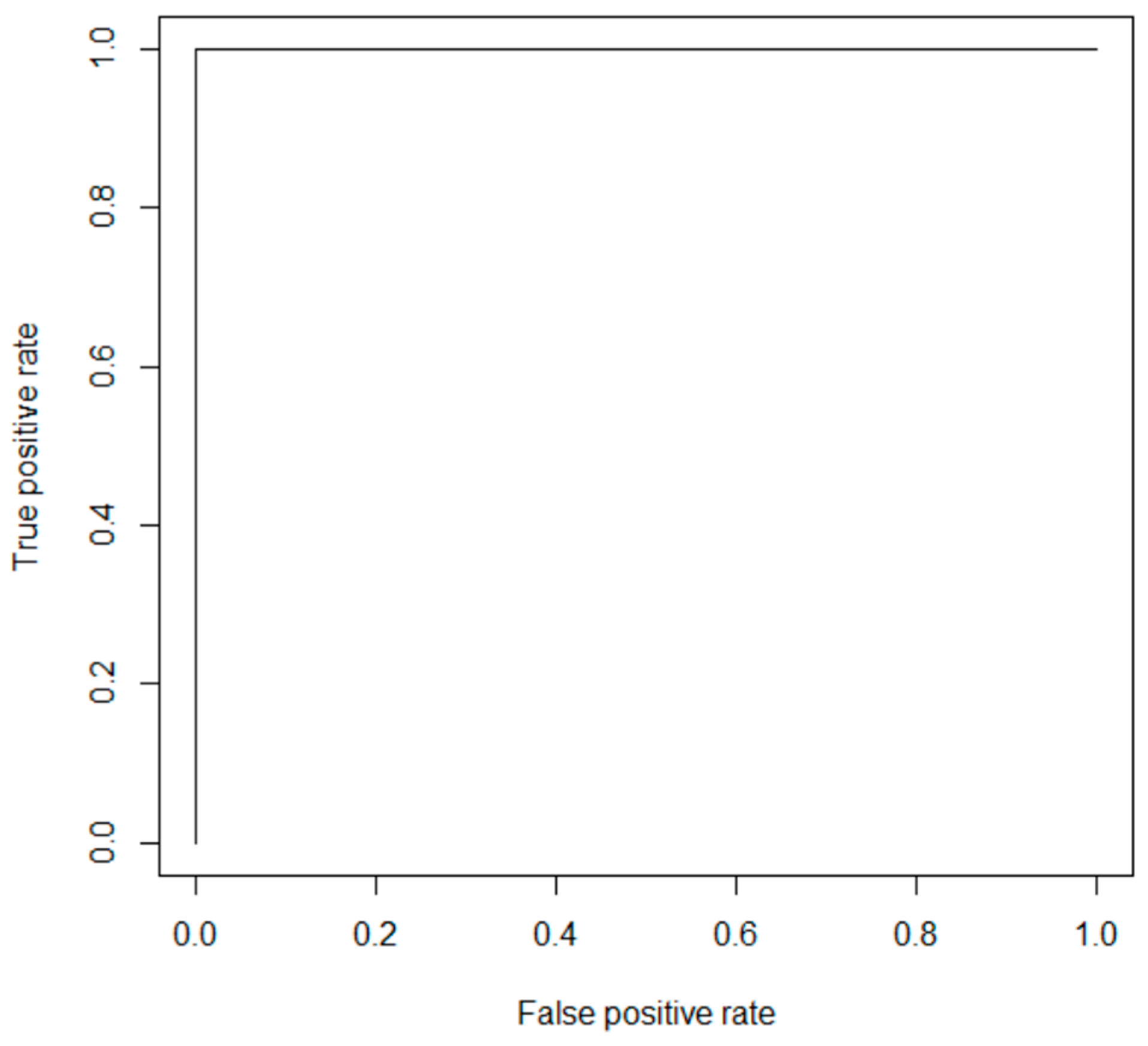
| cnn-ker-seg11 | 4 | 1.0000 | 1.0000 |
| cnn-mxn-ori12 | 6 | 0.9910 | 0.9920 |
| cnn-mxn-seg13 | 3 | 0.9980 | 0.9982 |
| cnn-mxn-ori14 | 4 | 1.0000 | 1.0000 |
| cnn-mxn-seg15 | 4 | 1.0000 | 1.0000 |
| Test Label | Epochs | Time [ms] | Memory [MB] |
|---|---|---|---|
| cnn-ker-ori10 | 5 | 38,610 | 186.9 |
| cnn-ker-seg11 | 4 | 30,660 | 180.0 |
| cnn-mxn-ori12 | 6 | 119,630 | 4.7 |
| cnn-mxn-seg13 | 3 | 82,580 | 2.6 |
| cnn-mxn-ori14 | 4 | 12,170 | 157.9 |
| cnn-mxn-seg15 | 4 | 11,850 | 3.7 |
| Test Label | Image Time Preparation [ms] | Diagnostic Time [ms] | Memory [MB] |
|---|---|---|---|
| mlp-rsn-sum04 | 210 | 20 | 0.2 |
| mlp-rsn-hpr05 | 194 | 240 | 3.0 |
| mlp-rsn-pol06 | 198 | 105 | 1.8 |
| cnn-mxn-ori14 | 14 | 14 | 0.5 |
| cnn-mxn-seg15 | 194 | 4 | 0.5 |
© 2019 by the authors. Licensee MDPI, Basel, Switzerland. This article is an open access article distributed under the terms and conditions of the Creative Commons Attribution (CC BY) license (http://creativecommons.org/licenses/by/4.0/).
Share and Cite
Haffner, O.; Kučera, E.; Drahoš, P.; Cigánek, J. Using Entropy for Welds Segmentation and Evaluation. Entropy 2019, 21, 1168. https://doi.org/10.3390/e21121168
Haffner O, Kučera E, Drahoš P, Cigánek J. Using Entropy for Welds Segmentation and Evaluation. Entropy. 2019; 21(12):1168. https://doi.org/10.3390/e21121168
Chicago/Turabian StyleHaffner, Oto, Erik Kučera, Peter Drahoš, and Ján Cigánek. 2019. "Using Entropy for Welds Segmentation and Evaluation" Entropy 21, no. 12: 1168. https://doi.org/10.3390/e21121168
APA StyleHaffner, O., Kučera, E., Drahoš, P., & Cigánek, J. (2019). Using Entropy for Welds Segmentation and Evaluation. Entropy, 21(12), 1168. https://doi.org/10.3390/e21121168