Abstract
Identifying brain regions contained in brain functional networks and functions of brain functional networks is of great significance in understanding the complexity of the human brain. The 160 regions of interest (ROIs) in the human brain determined by the Dosenbach’s template have been divided into six functional networks with different functions. In the present paper, the complexity of the human brain is characterized by the sample entropy (SampEn) of dynamic functional connectivity (FC) which is obtained by analyzing the resting-state functional magnetic resonance imaging (fMRI) data acquired from healthy participants. The 160 ROIs are clustered into six clusters by applying the K-means clustering algorithm to the SampEn of dynamic FC as well as the static FC which is also obtained by analyzing the resting-state fMRI data. The six clusters obtained from the SampEn of dynamic FC and the static FC show very high overlap and consistency ratios with the six functional networks. Furthermore, for four of six clusters, the overlap ratios corresponding to the SampEn of dynamic FC are larger than that corresponding to the static FC, and for five of six clusters, the consistency ratios corresponding to the SampEn of dynamic FC are larger than that corresponding to the static FC. The results show that the combination of machine learning methods and the FC obtained using the blood oxygenation level-dependent (BOLD) signals can identify the functional networks of the human brain, and nonlinear dynamic characteristics of the FC are more effective than the static characteristics of the FC in identifying brain functional networks and the complexity of the human brain.
1. Introduction
The human brain shows complex spatiotemporal behaviors when executing physiological functions. Characterizing dynamics of the complex spatiotemporal behaviors is of great significance in understanding the human brain. Since blood oxygenation level-dependent (BOLD) signals of different brain regions can be measured by the functional magnetic resonance imaging (fMRI) technique at high spatial and temporal resolutions, BOLD signals have been widely used to characterize dynamics of the spatiotemporal behaviors of the human brain [1,2]. For instance, the temporal correlation in BOLD signals of two distinct brain regions is commonly employed to describe the functional connectivity (FC) between them [3]. A positive and strong temporal correlation corresponds to a strong FC, and some brain regions with strong FCs among them constitute a brain functional network [4,5,6]. Alterations of some FCs in a brain functional network are often associated with brain disorder, such as schizophrenia [7], major depression [8], autism [9], Alzheimer’s Disease [10], and attention deficit hyperactivity disorder [11]. For example, Cheng et al. evaluated the FC between different brain regions in subjects with autism and found a key system in the middle temporal gyrus with reduced FC and a key system in the precuneus with reduced FC [12].
In most previous research on FC, only one correlation coefficient is acquired using entire BOLD signals of two distinct brain regions. The one correlation coefficient is called the static FC between the two brain regions. Recently, to understand dynamics of the spatiotemporal behaviors of the human brain more deeply, some researchers acquired a sequence of correlation coefficients by applying the sliding-window approach to BOLD signals of two distinct brain regions [13,14,15,16,17,18,19,20,21,22,23]. These correlation coefficients form a time series which is called the dynamic FC between the two brain regions. The dynamic FC exhibits complex characteristics which are effective in describing properties of the brain functional networks of patients with brain disorder. For instance, in one of our recent studies, complex characteristics of dynamic FC were described by sample entropy (SampEn), and the effects of schizophrenia on such complex characteristics were investigated. It was shown that the visual cortex of the patients with schizophrenia exhibited significantly higher SampEn than that of the healthy controls [24]. As introduced above, both the static FC and the SampEn of dynamic FC are effective in describing properties of the brain functional networks of patients with brain disorder. However, the effectivenesses of the static FC and the dynamic FC have not been compared directly.
Studies on the static FC or the dynamic FC are often carried out by first extracting BOLD signals of different brain regions and then evaluating the static or the dynamic FC between different brain regions for further analysis. Different brain regions are often determined by a brain template, such as the Dosenbach’s template [25]. The Dosenbach’s template includes 160 regions of interest (ROIs) determined by a sequence of meta-analyses of task-based fMRI studies which cover much of the human brain [
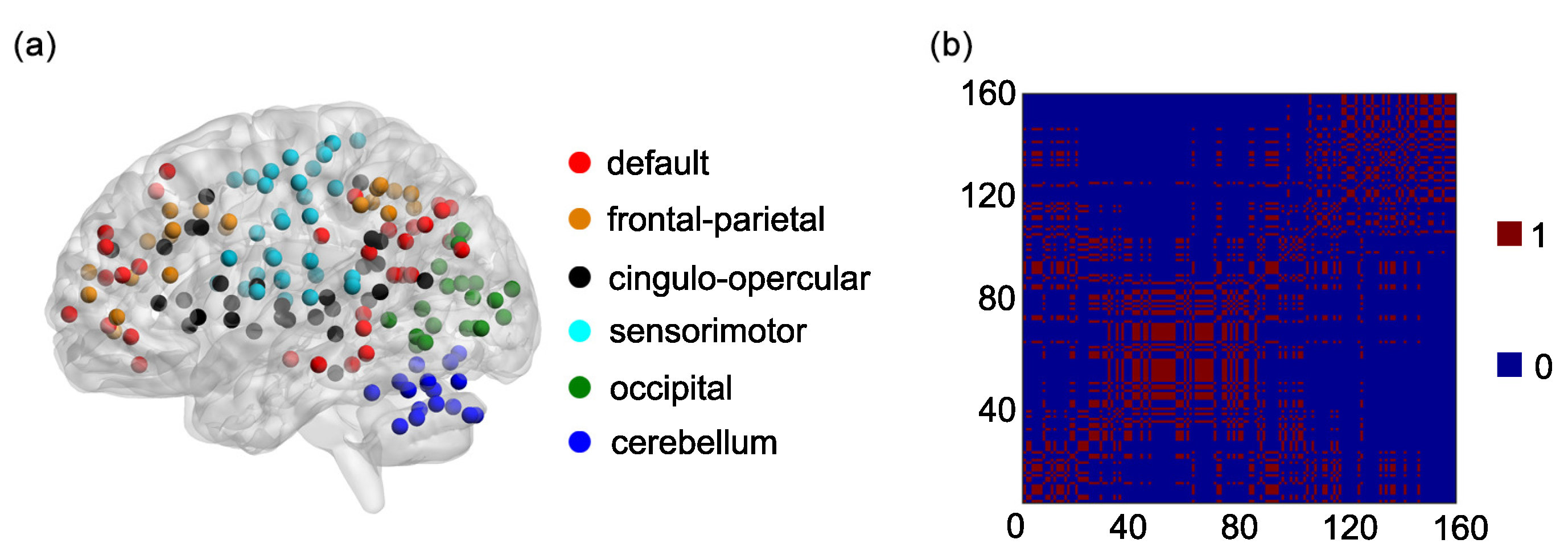
25]. Furthermore, the 160 ROIs can be separated into six functional networks including the default, the frontal-parietal, the cingulo-opercular, the sensorimotor, the occipital, and the cerebellum networks, which were identified by performing modularity optimization on the average FC matrix across a large cohort of healthy subjects [25]. The six functional networks have been used in predicting brain maturity across development [25,26], parcellating cortical or subcortical regions [27], examining the influence of temporal properties of BOLD signals on FC [28] and so on. For instance, Zhong et al. parcellated the hippocampus based on the FC, and showed that both the left and right hippocampus were divided into three subregions exhibiting different FC profiles with the six functional networks [27]. However, machine learning algorithms have not been used to identify the six functional networks.
The K-means clustering algorithm is one of the unsupervised learning algorithms [29]. Since the K-means clustering algorithm can cluster different observations into different clusters in a simple and easy way, it has been widely used in fMRI studies [30,31,32,33,34,35,36,37,38]. For instance, Fan et al. used the K-means clustering algorithm to parcellate the thalamus based on the static FC and found that the thalamus could be divided into seven symmetric thalamic clusters [36]. Park et al. parcellated the primary and secondary visual cortices (V1 and V2) into several subregions by applying the K-means clustering algorithm to the static FC and found that V1 and V2 could be separated into anterior and posterior subregions [38].
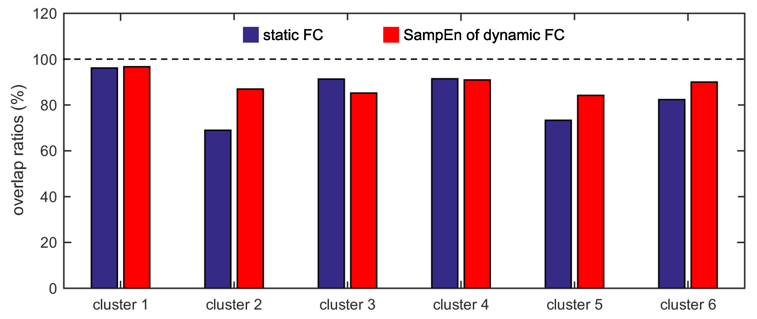
The present study intends to cluster the Dosenbach’s 160 ROIs into six clusters by applying the K-means clustering algorithm to the static FC and the SampEn of dynamic FC, to analyze the overlap and consistency between the six clusters and the six functional networks, and to compare the effectivenesses of the static FC and the dynamic FC. It is shown that applying the K-means clustering algorithm to FC is feasible to identify the six functional networks, and the SampEn of dynamic FC is more effective than the static FC as the six clusters obtained from the SampEn of dynamic FC show higher overlap and consistency ratios with the six functional networks.
This paper is organized as follows. The experiments and methods are presented in Section 2. The cluster results for the static FC and the SampEn of dynamic FC and the comparisons between them are shown in Section 3. The conclusion and discussion are described in Section 4. Some supplementary tables are presented in the appendix.
2. Experiments and Methods
2.1. Participants
FMRI data for this study were acquired at Olin Neuropsychiatry Research Center and have been made publicly available http://fcon_1000.projects.nitrc.org/indi/abide. The data were acquired from 31 healthy participants (18 males and 13 females) over the age range 18–30 years. This sample was retained after applying criteria for head motion, from a total of 35 healthy participants. Informed consent was obtained from all participants in accordance with Olin Neuropsychiatry Research Center Institutional Review Board oversight.
2.2. Data Acquisition and Preprocessing
BOLD signals are extracted from three-dimensional functional images collected on a Siemens 3T MRI scanner with the following parameters: repetition time (TR), 475 ms; echo time, 30 ms; field of view, ; slices, 48; slice thickness, 3 mm; flip angle, . During the data collection, all participants were instructed to rest but not fall asleep. For each participant, 947 three-dimensional functional images were collected.
The functional images are preprocessed using SPM8 and DPABI softwares [39,40]. Firstly, the first 4 images are discarded to reduce the negative effects of scanner’s stabilization on the analysis results. Secondly, the images are corrected for time delay in slice acquisition and rigid-body head motion. Thirdly, several confounding factors are regressed out from the images, including 6 head motion parameters and the cerebrospinal, the white matter, and the global brain signals. Fourthly, temporal band-pass filtering (0.01–0.08 Hz) of the images are performed to reduce the negative effects of low-frequency drift and high-frequency physiological noise on the analysis results. Fifthly, the images are spatially normalized to the Montreal Neurological Institute space and are resampled to voxels of size . Sixthly, the images are smoothed with a Gaussian kernel of 8 mm full-width at half-maximum. Finally, the BOLD signal of each voxel is extracted from the functional images.
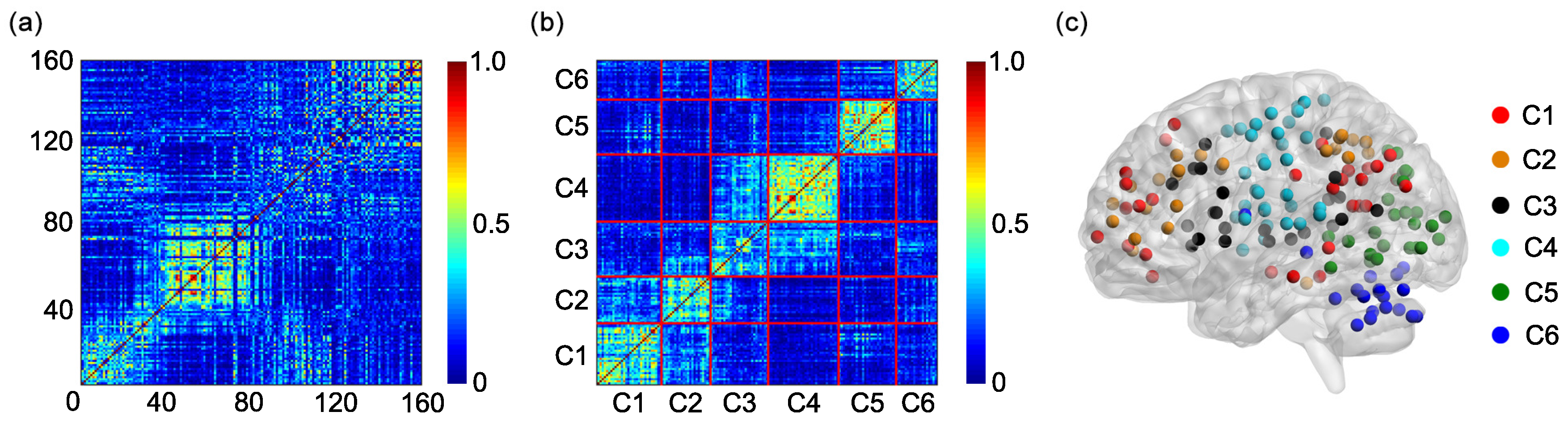
2.3. The Dosenbach’s Template and the 6 Functional Networks
One hundred and sixty regions of interest (ROIs) are selected based on the Dosenbach’s template [25]. The centroid of each ROI is derived from a sequence of meta-analyses of task-based fMRI studies (Figure 1a). The radius of each ROI equals 5 mm (Figure 1a). The name and the sequential number of each ROI can be found in Table A1 in Appendix A. The 160 ROIs can further be grouped into 6 functional networks, including the default, the frontal-parietal, the cingulo-opercular, the sensorimotor, the occipital, and the cerebellum networks (Figure 1a). The name and the sequential number of each ROI in each functional network can be found in the first and second columns of Table A2, Table A3, Table A4, Table A5, Table A6 and Table A7 in Appendix A.
Figure 1.
(a) One hundred and sixty regions of interest (ROIs) are shown on a surface rendering of the brain. ROIs in different functional networks are shown in different colors. (b) The adjacent matrix A of 160 ROIs in 6 functional networks.
Based on the 6 functional networks, an adjacent matrix can be generated [36,41,42]. The adjacent matrix is labeled as
Each of the elements on the main diagonal of A is 1. Other elements of A are defined as follows: if the ith ROI and the jth ROI are contained in the same functional network and otherwise (Figure 1b).
2.4. The Static FC and the Dynamic FC
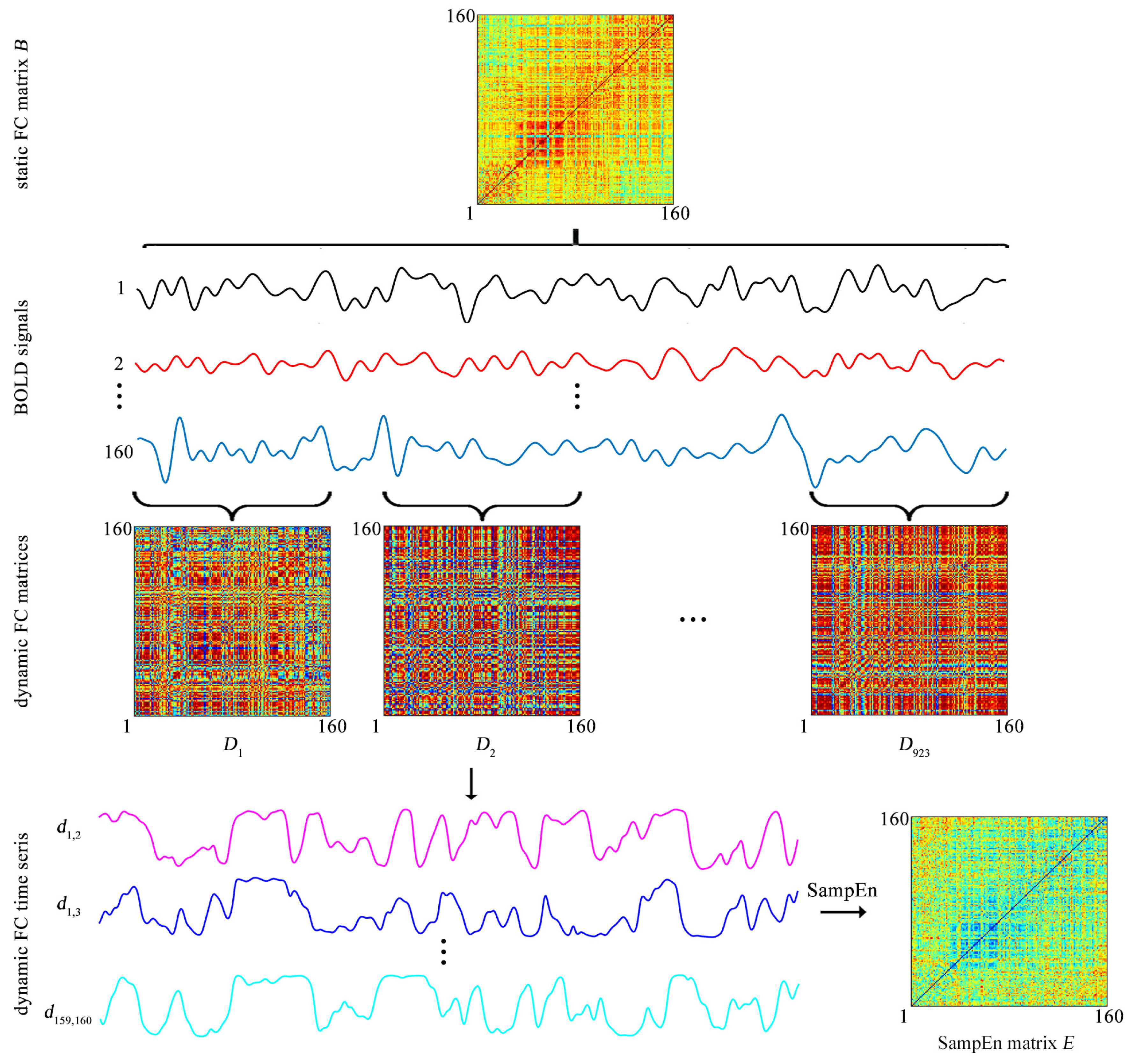
The BOLD signal of each ROI is extracted by averaging the BOLD signals over all voxels in this ROI. Then both the static FC and the dynamic FC are evaluated (Figure 2).
Figure 2.
The static functional connectivity (FC) matrix B and the SampEn matrix E obtained from the BOLD signals of 160 ROIs. The matrices B and E are used to cluster the 160 ROIs into 6 clusters by the K-means clustering algorithm.
The static FC between each pair of ROIs is assessed by a Pearson correlation coefficient. For each of the 31 participants, after the static FC between each pair of ROIs is evaluated, a static FC matrix of size is obtained (Figure 2), which is labeled as
The ith row represents the static FC between the ith ROI and all the other ROIs The matrix B is used to cluster the 160 ROIs into 6 clusters.
Dynamic FC is assessed by the sliding-window approach. Specifically, a tapered window is created by convolving a rectangle window (size = 20 TRs = 9.5 s) with a Gaussian curve (standard deviation = 3 TRs) [14,15,23]. The window is used to extract BOLD signals in a step of 1 TR, leading to 923 time windows per subject (Figure 2). For the kth time window a Pearson correlation coefficient is used to evaluate the FC between each pair of ROIs and thus a FC matrix of size which is labeled as
which is obtained for each subject (Figure 2). As k increases from 1 to 923, forms a time series which represents the temporal evolution of the FC between the ith and jth ROIs and is named as the dynamic FC (Figure 2). Since previous studies showed that the window of size 20 TRs captures more transient patterns in dynamic FC [23], the window size is fixed at 20 TRs throughout the study.
2.5. SampEn of a Dynamic FC Time Series
For each dynamic FC time series, the SampEn is calculated. For convenience, time series is denoted by SampEn of is computed as follows [24,43,44,45,46].
Firstly, constructing embedding vectors in which m stands for the dimension of
Secondly, define
r stands for a tolerance value which is defined as , where is a small parameter and is the standard deviation of . , the Heaviside function, which is defined as
represents the Chebyshev distance, i.e.,
Similarly, define
Finally, calculate SampEn of as
The value of SampEn is not less than 0, and a larger value of SampEn means more complexity [47]. Similar to our previous study [24,43], m and are fixed at 2 and 0.2, respectively.
In addition, because the SampEn of equals 0 Thus, for each participant, a SampEn matrix of size is obtained (Figure 2). The SampEn matrix is labeled as
The element represents the SampEn of dynamic FC between the ith ROI and jth ROI equals 0 The matrix E is used to cluster the 160 ROIs into 6 clusters.
2.6. Clustering ROIs into 6 Clusters by Applying the K-Means Clustering Algorithm to the Static FC Matrix
For each of the 31 participants, there exists a static FC matrix B of size The ith row represents the static FC between the ith ROI and all the other ROIs.
The K-means clustering algorithm is commonly used to cluster different observations into different clusters based on the distance between these observations [29]. In the present paper, the K-means clustering algorithm is applied to the matrix B to cluster 160 ROIs into 6 clusters. Procedures of the algorithm are briefly described as follows.
First, select 6 rows from the matrix B and use these 6 rows as initial cluster centroids.
Secondly, calculate the squared Euclidean distance between each row and each initial cluster centroid, and then assign each row to the cluster with the closest centroid.
Thirdly, when all rows have been assigned, calculate the average of the rows in each cluster to obtain 6 new cluster centroids.
Finally, repeat the second and the third steps until the centroids no longer change.
The algorithm generates 6 clusters, and each cluster is composed of different rows of the matrix B (or of different ROIs). Based on the 6 clusters, an individual adjacent matrix of size is generated [36,41,42]. The individual adjacent matrix is labeled as
Each of the elements on the main diagonal of F is 1, and other elements of F are defined as follows: if the ith ROI and the jth ROI are contained in the same cluster and otherwise.
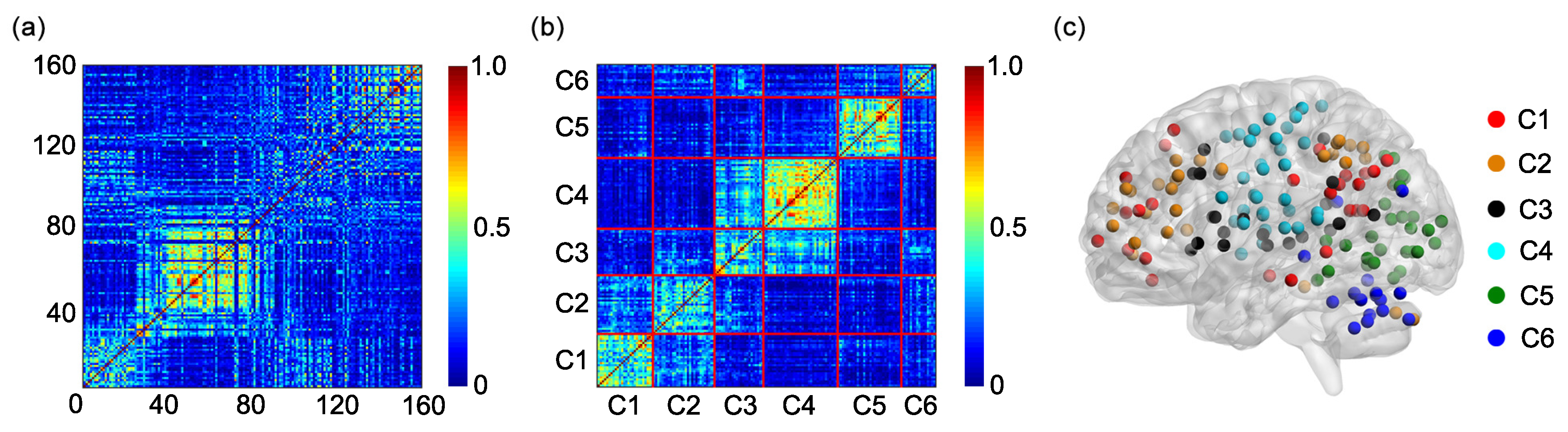
Since the study includes 31 participants, 31 individual adjacent matrices are obtained. A group adjacent matrix of size is obtained by averaging 31 individual adjacent matrices. The group adjacent matrix is labeled as
The K-means clustering algorithm is further applied to the matrix G to obtain the group cluster result [36,41,42] and the 6 clusters of the group cluster result are compared with the 6 functional networks shown in Figure 1a.
The detailed clustering procedure is performed by MATLAB software (MATLAB R2014b). Considering that the K-means clustering algorithm is sensitive to the initial cluster centroids, we repeat each clustering procedure 500 times, and the cluster result with the lowest within-cluster distance is adopted.
2.7. Clustering ROIs into 6 Clusters by Applying the K-Means Clustering Algorithm to the SampEn Matrix
The procedures described in Section 2.6 are also applied to the SampEn matrix E, and 6 clusters are obtained.
3. Results
3.1. Six Clusters of ROIs for the Static FC
The group adjacent matrix for the static FC is shown in Figure 3a. The horizontal and vertical coordinates represent the sequential numbers of the ROIs. The sequential number and the name of each ROI can be found in Table A1 in Appendix A.
Figure 3.
(a) The group adjacent matrix for the static FC. (b) The reorganization of the group adjacent matrix based on the 6 clusters obtained by applying the K-means clustering algorithm to the group adjacent matrix. Since the ith row and the ith column of the group adjacent matrix are reorganized simultaneously, the reorganized matrix is also symmetric. (c) The 6 clusters are shown on a surface rendering of the brain. C1: cluster 1; C2: cluster 2; C3: cluster 3; C4: cluster 4; C5: cluster 5; C6: cluster 6.
Rows of the group adjacent matrix can be clustered into six clusters by the K-means clustering algorithm (Figure 3b). The numbers of rows in clusters 1–6 are 26, 29, 23, 35, 30, and 17, respectively (Table 1). The ROIs in clusters 1–6 can be found in the third and fourth columns of Table A2, Table A3, Table A4, Table A5, Table A6 and Table A7 in Appendix A. Since each row of the adjacent matrix corresponds to a ROI, the six clusters can also be shown on a surface rendering of the brain (Figure 3c), which resembles Figure 1a to a large extent.
Table 1.
The number of ROIs in the overlapping part between each functional network and each cluster obtained from the static FC.
The average of the squared Euclidean distances from all ROIs in each of the six clusters to the centroid of cluster is also evaluated, as shown in Figure 4a–f. For each centroid, among the six averaged distances, the averaged distance from the cluster to the centroid of cluster i is the lowest. This is consistent with the main idea of the K-means clustering algorithm.
Figure 4.
The average of the squared Euclidean distances from all ROIs in each of the six clusters to the centroid of cluster . (a) Centroid of cluster 1. (b) Centroid of cluster 2. (c) Centroid of cluster 3. (d) Centroid of cluster 4. (e) Centroid of cluster 5. (f) Centroid of cluster 6. The error bars represent standard deviations.
3.2. The Overlap Ratios between the Six Clusters for the Static FC and the Six Functional Networks
The overlap ratios between each cluster and each functional network is analyzed in Table 1. The overlap ratios between cluster 1 and the default network, the frontal-parietal network, the cingulo-opercular network, the sensorimotor network, the occipital network, as well as the cerebellum network are 25/26 (≈96.15%), 0, 1/26 (≈3.85%), 0, 0, and 0, respectively. Obviously, the overlap ratio between cluster 1 and the default network is the highest. Thus, cluster 1 corresponds to the default network. Similarly, we can obtain that clusters 2–6, respectively, correspond to the frontal-parietal network, the cingulo-opercular network, the sensorimotor network, the occipital network, and the cerebellum network, with the overlap ratios, respectively, equaling 20/29 (≈68.97%), 21/23 (≈91.30%), 32/35 (≈91.43%), 22/30 (≈73.33%), and 14/17 (≈82.35%). These overlap ratios are high.
3.3. The Consistency Ratios between the Six Clusters for the Static FC and the Functional Networks
Based on the data shown in Table 1, the consistency between the cluster results and the functional networks can also be evaluated. The consistency ratio between cluster 1 and the default network is 25/(25 + 9 + 1) (≈71.43%), in which 9 is the number of ROIs in the default network but not in cluster 1, and 1 is the number of ROIs in cluster 1 but not in the default network. Similarly, we can obtain that the consistency ratios between cluster 2 and the frontal-parietal network, cluster 3 and the cingulo-opercular network, cluster 4 and the sensorimotor network, cluster 5 and the occipital network, and cluster 6 and the cerebellum network are 20/(20 + 1 + 9) (≈66.67%), 21/(21 + 11 + 2) (≈61.76%), 32/(32 + 1 + 3) (≈88.89%), 22/(22 + 0 + 8) (≈73.33%), and 14/(14 + 4 + 3) (≈66.67%), respectively. These consistency ratios are high.
3.4. Six Clusters of ROIs for the SampEn of Dynamic FC
The group adjacent matrix for the SampEn of dynamic FC is presented in Figure 5a. The horizontal and vertical coordinates stand for the sequential numbers of the ROIs. The sequential number and the name of each ROI can be found in Table A1 in Appendix A.
Figure 5.
(a) The group adjacent matrix for the SampEn of dynamic FC. (b) The reorganization of the group adjacent matrix based on the six clusters obtained by applying the K-means clustering algorithm to the group adjacent matrix. Since the ith row and the ith column of the group adjacent matrix are reorganized simultaneously, the reorganized matrix is also symmetric. (c) The six clusters are shown on a surface rendering of the brain. C1: cluster 1; C2: cluster 2; C3: cluster 3; C4: cluster 4; C5: cluster 5; C6: cluster 6.
Rows of the group adjacent matrix can be divided into six clusters by the K-means clustering algorithm (Figure 5b). The numbers of rows in clusters 1–6 are 30, 23, 27, 33, 27, and 20, respectively (Table 2). The ROIs in clusters 1–6 can be found in the fifth and sixth columns of Table A2, Table A3, Table A4, Table A5, Table A6 and Table A7 in Appendix A. The six clusters can also be shown on a surface rendering of the brain (Figure 5c), which resembles Figure 1a and Figure 3c to a large extent.
Table 2.
The number of ROIs in the overlapping part between each functional network and each cluster obtained from the SampEn of dynamic FC.
Furthermore, other values of are also tried in the K-means clustering algorithm, and the optimal value of K is determined by the elbow criterion of the cluster validity index, which is defined as the ratio of within-cluster distances to between-cluster distances [15,20,27]. The dependence of the cluster validity index on K is shown in Figure 6. It is seen that two elbows appear at 4 and 6 due to the changes of slopes of the trend lines. Thus, the optimal values of K are 4 and 6. In order to compare the cluster results with the six functional networks already discussed in the literature [25], K is fixed at 6 in the present paper.
Figure 6.
The dependence of the cluster validity index on K. The thin solid, dotted, and bold solid lines are trend lines of the filled circles. Since slopes of the trend lines change significantly at 4 and 6, based on the elbow criterion, the optimal values of K are 4 and 6.
The average of the squared Euclidean distances from all ROIs in each of the six clusters to the centroid of cluster is calculated, as shown in Figure 7a–f. For each centroid, among the six averaged distances, the averaged distance from the cluster to the centroid of cluster i is the lowest. This is also in line with the main idea of the K-means clustering algorithm.
Figure 7.
The average of the squared Euclidean distances from all ROIs in each of the six clusters to the centroid of cluster (a) Centroid of cluster 1. (b) Centroid of cluster 2. (c) Centroid of cluster 3. (d) Centroid of cluster 4. (e) Centroid of cluster 5. (f) Centroid of cluster 6. The error bars represent standard deviations.
3.5. The Overlap Ratios between the Six Clusters for the SampEn of Dynamic FC and the Six Functional Networks
The overlap ratio between each cluster and each functional network is analyzed in Table 2. By evaluating the overlap ratio between each cluster and each functional network, we find that clusters 1–6, respectively, correspond to the default network, the frontal-parietal network, the cingulo-opercular network, the sensorimotor network, the occipital network, and the cerebellum network, with the overlap ratios, respectively, equaling 29/30 (≈96.67%), 20/23 (≈86.96%), 23/27 (≈85.19%), 30/33 (≈90.91%), 22/27 (≈81.48%), and 18/20 (≈90.00%). These overlap ratios are very high.
3.6. The Consistency Ratios between the Six Clusters for the SampEn of Dynamic FC and the Six Functional Networks
Based on the data shown in Table 2, the consistency ratios between the six clusters obtained from the SampEn of dynamic FC and the six functional networks are evaluated. The consistency ratios between cluster 1 and the default network, cluster 2 and the frontal-parietal network, cluster 3 and the cingulo-opercular network, cluster 4 and the sensorimotor network, cluster 5 and the occipital network, and cluster 6 and the cerebellum network are 29/(29 + 5 + 1) (≈82.86%), 20/(20 + 1 + 3) (≈83.33%), 23/(23 + 9 + 4) (≈63.89%), 30/(30 + 3 + 3) (≈83.33%), 22/(22 + 0 + 5) (≈81.48%), and 18/(18 + 0 + 2) (≈90.00%), respectively. These consistency ratios are very high.
3.7. The SampEn of Dynamic FC is More Effective Than the Static FC
For the two different measurements (the static FC and the SampEn of dynamic FC), the overlap ratios between cluster 1 and the default network, cluster 2 and the frontal-parietal network, cluster 3 and the cingulo-opercular network, cluster 4 and the sensorimotor network, cluster 5 and the occipital network, and cluster 6 and the cerebellum network are shown in Figure 8. For cluster 3, the overlap ratio corresponding to the static FC (91.30%) is larger than that corresponding to the SampEn of dynamic FC (85.19%). For cluster 4, the overlap ratio corresponding to the static FC (91.43%) is slightly larger than that corresponding to the SampEn of dynamic FC (90.91%). For the other four clusters (clusters 1, 2, 5, and 6), the overlap ratios corresponding to the SampEn of dynamic FC are larger than that corresponding to the static FC. For clusters 1, 2, 5, and 6, the overlap ratios corresponding to the SampEn of dynamic FC are 96.67%, 86.96%, 81.48%, and 90.00%, whereas the overlap ratios corresponding to the static FC are 96.15%, 68.97%, 73.33%, and 82.35%.
Figure 8.
The overlap ratios between cluster 1 and the default network, cluster 2 and the frontal-parietal network, cluster 3 and the cingulo-opercular network, cluster 4 and the sensorimotor network, cluster 5 and the occipital network, and cluster 6 and the cerebellum network for the two different measurements.
For the two different measurements, the consistency ratios between cluster 1 and the default network, cluster 2 and the frontal-parietal network, cluster 3 and the cingulo-opercular network, cluster 4 and the sensorimotor network, cluster 5 and the occipital network, and cluster 6 and the cerebellum network are shown in Figure 9. For cluster 4, the consistency ratio corresponding to the static FC (88.89%) is larger than that corresponding to the SampEn of dynamic FC (83.33%). For the other five clusters, the consistency ratios corresponding to the SampEn of dynamic FC are larger than that corresponding to the static FC. For clusters 1, 2, 3, 5, and 6, the consistency ratios corresponding to the SampEn of dynamic FC are 82.86%, 83.33%, 63.89%, 81.48%, and 90.00%, whereas the consistency ratios corresponding to the static FC are 71.43%, 66.67%, 61.76%, 73.33%, and 66.67%.
Figure 9.
The consistency ratios between cluster 1 and the default network, cluster 2 and the frontal-parietal network, cluster 3 and the cingulo-opercular network, cluster 4 and the sensorimotor network, cluster 5 and the occipital network, and cluster 6 and the cerebellum network for the two different measurements.
According to the results shown in Figure 8 and Figure 9, we conclude that the SampEn of dynamic FC is more effective than the static FC in clustering different ROIs into different functional networks. This phenomenon can be interpreted by evaluating the similarity between the adjacent matrix generated based on the six functional networks (Figure 1b) and the group adjacent matrix for the static FC (Figure 3a) or for the SampEn of dynamic FC (Figure 5a). The similarity is evaluated by the squared Euclidean distance, and a smaller distance means more similarity. The distances from the adjacent matrix shown in Figure 1b to the group adjacent matrices shown in Figure 3a and in Figure 5a are 2409.58 and 2376.52, respectively. The latter is smaller than the former, i.e., the similarity between the adjacent matrix shown in Figure 1b and the group adjacent matrix shown in Figure 5a is larger than the similarity between the adjacent matrix shown in Figure 1b and the group adjacent matrix shown in Figure 3a. This causes the SampEn of dynamic FC to be more effective than the static FC in clustering different ROIs into different functional networks.
4. Conclusions and Discussion
Different brain regions in the human brain functionally interact with each other to construct multiple functional networks. Identifying the function of each functional network and the brain regions contained in each functional network is very important for understanding the human brain. The present study tests the feasibility of using the K-means clustering algorithm to identify the functional networks based on the FC, including the static FC and the dynamic FC. By applying the K-means clustering algorithm to the static FC or the SampEn of dynamic FC between different ROIs determined by the Dosenbach’s template, we show that the Dosenbach’s 160 ROIs can be divided into six clusters which show high overlap and consistency ratios with the six functional networks identified by applying modularity optimization on the average FC matrix across a large cohort of healthy subjects. The results indicate that the combination of the K-means clustering algorithm and the FC can identify the functional networks of the human brain. The K-means algorithm has been commonly used to parcellate cortical or subcortical regions based on the static FC [30,31,32,33,34,35,36,37,38]. These previous studies along with the present study extend the application of machine learning methods in brain sciences.
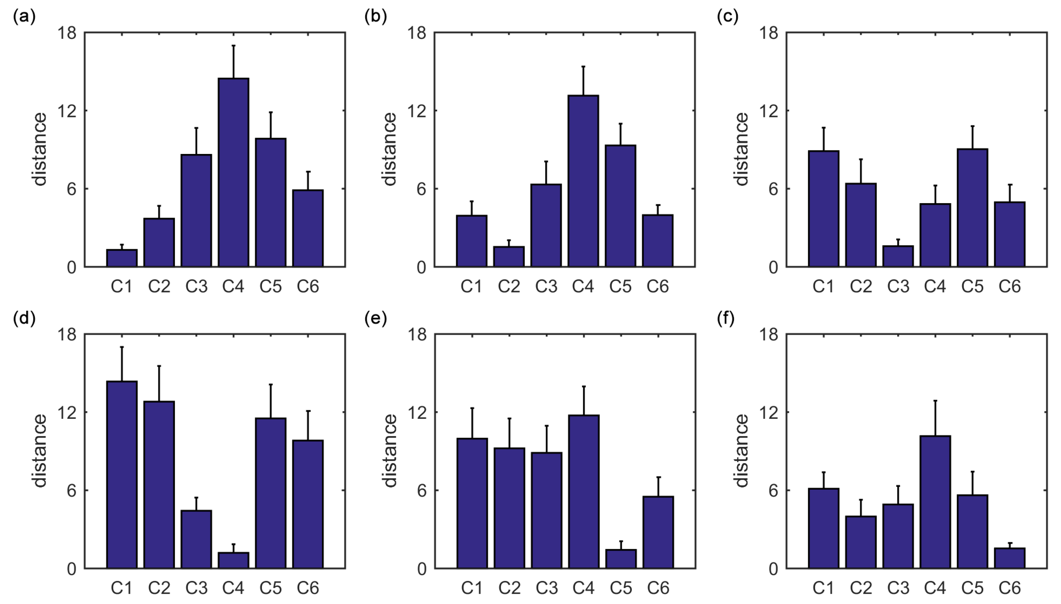
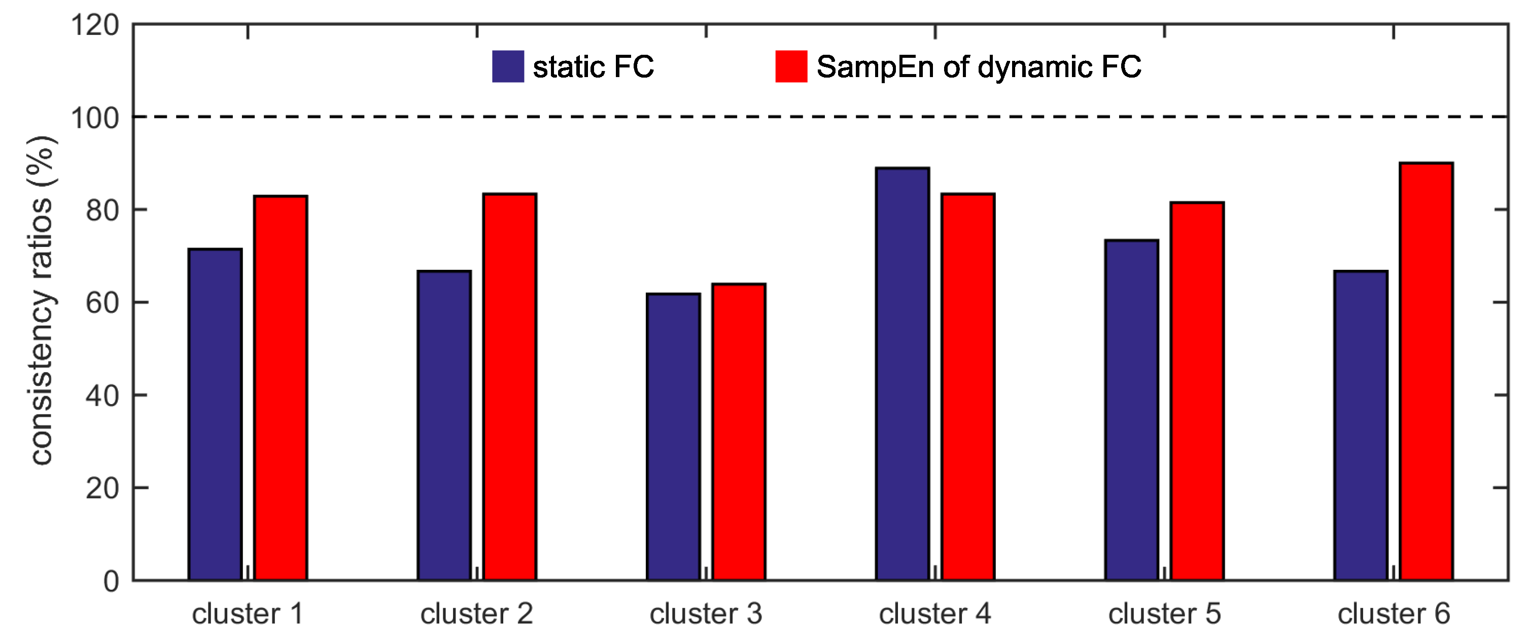
Furthermore, we show that, for four of six clusters, the overlap ratios corresponding to the SampEn of dynamic FC are larger than that corresponding to the static FC, and for five of six clusters, the consistency ratios corresponding to the SampEn of dynamic FC are larger than that corresponding to the static FC. This indicates that nonlinear dynamic characteristics of the FC is more effective than the static characteristics of the FC in identifying brain functional networks. In our previous studies, by characterizing the nonlinear characteristics of dynamic FC in healthy subjects and patients with schizophrenia, we have shown that SampEn of the amygdala-cortical FC in healthy subjects decreased with age increasing, and the visual cortex of the patients with schizophrenia exhibited significantly higher SampEn than that of the healthy subjects [24,43]. In the future, nonlinear characteristics of dynamic FC should be deeply used to characterize properties of brain functional networks and the complexity of the human brain.
Author Contributions
Conceptualization, Y.J. and H.G.; Data curation, Y.J.; Formal analysis, Y.J. and H.G.; Funding acquisition, Y.J. and H.G.; Investigation, Y.J. and H.G.; Methodology, Y.J. and H.G.; Resources, Y.J. and H.G.; Software, Y.J.; Supervision, H.G.; Visualization, Y.J.; Writing-original draft, Y.J.; Writing-review & editing, H.G.
Funding
This research was funded by the National Natural Science Foundation of China (Grant Nos: 11802086, 11872276, and 11572225) and the Scientific and Technological Project of Henan Province (Grant No: 192102210263).
Acknowledgments
We would like to thank www.nitrc.org for allowing us to access the database used in this work.
Conflicts of Interest
The authors declare no conflict of interest.
Appendix A
Table A1.
The names and the sequential numbers of 160 ROIs.
Table A1.
The names and the sequential numbers of 160 ROIs.
| No. | Name | No. | Name | No. | Name | No. | Name |
|---|---|---|---|---|---|---|---|
| 1 | vmPFC | 41 | pre-SMA | 81 | fusiform | 121 | inf cerebellum |
| 2 | aPFC | 42 | vFC | 82 | temporal | 122 | inf cerebellum |
| 3 | aPFC | 43 | SMA | 83 | temporal | 123 | temporal |
| 4 | mPFC | 44 | mid insula | 84 | fusiform | 124 | angular gyrus |
| 5 | aPFC | 45 | frontal | 85 | precuneus | 125 | TPJ |
| 6 | vmPFC | 46 | precentral gyrus | 86 | sup parietal | 126 | occipital |
| 7 | vmPFC | 47 | thalamus | 87 | precuneus | 127 | med cerebellum |
| 8 | aPFC | 48 | mid insula | 88 | IPL | 128 | lat cerebellum |
| 9 | vent aPFC | 49 | precentral gyrus | 89 | parietal | 129 | occipital |
| 10 | vent aPFC | 50 | parietal | 90 | post cingulate | 130 | med cerebellum |
| 11 | vmPFC | 51 | precentral gyrus | 91 | inf temporal | 131 | inf cerebellum |
| 12 | vlPFC | 52 | precentral gyrus | 92 | occipital | 132 | precuneus |
| 13 | vmPFC | 53 | precentral gyrus | 93 | post cingulate | 133 | occipital |
| 14 | ACC | 54 | parietal | 94 | precuneus | 134 | IPS |
| 15 | vlPFC | 55 | mid insula | 95 | temporal | 135 | occipital |
| 16 | dlPFC | 56 | mid insula | 96 | IPL | 136 | occipital |
| 17 | sup frontal | 57 | thalamus | 97 | parietal | 137 | occipital |
| 18 | vPFC | 58 | thalamus | 98 | lat cerebellum | 138 | med cerebellum |
| 19 | ACC | 59 | mid insula | 99 | post parietal | 139 | occipital |
| 20 | sup frontal | 60 | temporal | 100 | sup temporal | 140 | inf cerebellum |
| 21 | ACC | 61 | mid insula | 101 | IPL | 141 | occipital |
| 22 | dlPFC | 62 | parietal | 102 | angular gyrus | 142 | occipital |
| 23 | vPFC | 63 | inf temporal | 103 | temporal | 143 | med cerebellum |
| 24 | dlPFC | 64 | parietal | 104 | IPL | 144 | med cerebellum |
| 25 | vFC | 65 | parietal | 105 | precuneus | 145 | occipital |
| 26 | ant insula | 66 | parietal | 106 | occipital | 146 | occipital |
| 27 | dACC | 67 | precentral gurus | 107 | IPL | 147 | occipital |
| 28 | ant insula | 68 | temporal | 108 | post cingulate | 148 | occipital |
| 29 | dFC | 69 | parietal | 109 | lat cerebellum | 149 | occipital |
| 30 | basal ganglia | 70 | post insula | 110 | inf cerebellum | 150 | inf cerebellum |
| 31 | mFC | 71 | basal ganglia | 111 | post cerebellum | 151 | inf cerebellum |
| 32 | frontal | 72 | inf temporal | 112 | precuneus | 152 | post occipital |
| 33 | vFC | 73 | post cingulate | 113 | lat cerebellum | 153 | post occipital |
| 34 | dFC | 74 | parietal | 114 | IPS | 154 | post occipital |
| 35 | dFC | 75 | parietal | 115 | post cingulate | 155 | inf cerebellum |
| 36 | dFC | 76 | post insula | 116 | IPS | 156 | post occipital |
| 37 | vFC | 77 | parietal | 117 | angular gyrus | 157 | post occipital |
| 38 | basal ganglia | 78 | temporal | 118 | occipital | 158 | post occipital |
| 39 | basal ganglia | 79 | post parietal | 119 | occipital | 159 | post occipital |
| 40 | vFC | 80 | post cingulate | 120 | med cerebellum | 160 | post occipital |
Table A2.
ROIs in the default network and in cluster 1 for the static FC and the SampEn of dynamic FC. ROIs in cluster 1 but not in the default network are marked by underlines.
Table A2.
ROIs in the default network and in cluster 1 for the static FC and the SampEn of dynamic FC. ROIs in cluster 1 but not in the default network are marked by underlines.
| Default Network | Cluster 1 for the Static FC | Cluster 1 for the SampEn | |||
|---|---|---|---|---|---|
| ROI 1 | ROI 92 | ROI 1 | ROI 1 | ||
| ROI 4 | ROI 93 | ROI 4 | ROI 93 | ROI 4 | ROI 93 |
| ROI 5 | ROI 94 | ROI 94 | ROI 5 | ROI 94 | |
| ROI 6 | ROI 105 | ROI 6 | ROI 105 | ROI 6 | ROI 105 |
| ROI 7 | ROI 108 | ROI 7 | ROI 108 | ROI 7 | ROI 108 |
| ROI 11 | ROI 111 | ROI 11 | ROI 111 | ROI 11 | ROI 111 |
| ROI 13 | ROI 112 | ROI 13 | ROI 112 | ROI 13 | ROI 112 |
| ROI 14 | ROI 115 | ROI 14 | ROI 115 | ROI 14 | ROI 115 |
| ROI 15 | ROI 117 | ROI 15 | ROI 117 | ROI 15 | ROI 117 |
| ROI 17 | ROI 124 | ROI 17 | ROI 124 | ROI 17 | ROI 124 |
| ROI 20 | ROI 132 | ROI 20 | ROI 20 | ||
| ROI 63 | ROI 134 | ROI 63 | ROI 134 | ROI 63 | ROI 134 |
| ROI 72 | ROI 136 | ROI 72 | ROI 72 | ||
| ROI 73 | ROI 137 | ROI 73 | ROI 73 | ROI 137 | |
| ROI 84 | ROI 141 | ROI 84 | |||
| ROI 85 | ROI 146 | ROI 85 | ROI 85 | ROI 146 | |
| ROI 90 | ROI 102 | ROI 102 | |||
| ROI 91 | ROI 91 | ROI 91 | |||
Table A3.
ROIs in the frontal-parietal network and in cluster 2 for the static FC and the SampEn of dynamic FC. ROIs in cluster 2 but not in the frontal-parietal network are marked by underlines.
Table A3.
ROIs in the frontal-parietal network and in cluster 2 for the static FC and the SampEn of dynamic FC. ROIs in cluster 2 but not in the frontal-parietal network are marked by underlines.
| Frontal-Parietal Network | Cluster 2 for the Static FC | Cluster 2 for the SampEn | |||
|---|---|---|---|---|---|
| ROI 2 | ROI 99 | ROI 2 | ROI 99 | ROI 2 | ROI 99 |
| ROI 3 | ROI 101 | ROI 3 | ROI 101 | ROI 3 | ROI 101 |
| ROI 9 | ROI 104 | ROI 9 | ROI 104 | ROI 9 | ROI 104 |
| ROI 10 | ROI 107 | ROI 10 | ROI 107 | ROI 10 | ROI 107 |
| ROI 12 | ROI 114 | ROI 12 | ROI 114 | ROI 12 | ROI 114 |
| ROI 16 | ROI 116 | ROI 16 | ROI 116 | ROI 16 | ROI 116 |
| ROI 21 | ROI 21 | ROI 5 | ROI 21 | ROI 8 | |
| ROI 22 | ROI 22 | ROI 8 | ROI 22 | ROI 18 | |
| ROI 23 | ROI 23 | ROI 18 | ROI 23 | ROI 81 | |
| ROI 24 | ROI 24 | ROI 19 | ROI 24 | ||
| ROI 29 | ROI 29 | ROI 25 | ROI 29 | ||
| ROI 34 | ROI 81 | ||||
| ROI 36 | ROI 36 | ROI 137 | ROI 36 | ||
| ROI 88 | ROI 88 | ROI 140 | ROI 88 | ||
| ROI 96 | ROI 96 | ROI 155 | ROI 96 | ||
Table A4.
ROIs in the cingulo-percular network and in cluster 3 for the static FC and the SampEn of dynamic FC. ROIs in cluster 3 but not in the cingulo-percular network are marked by underlines.
Table A4.
ROIs in the cingulo-percular network and in cluster 3 for the static FC and the SampEn of dynamic FC. ROIs in cluster 3 but not in the cingulo-percular network are marked by underlines.
| Cingulo-Percular Network | Cluster 3 for the Static FC | Cluster 3 for the SampEn | |||
|---|---|---|---|---|---|
| ROI 8 | ROI 61 | ROI 61 | ROI 61 | ||
| ROI 18 | ROI 71 | ROI 71 | ROI 71 | ||
| ROI 19 | ROI 76 | ROI 19 | |||
| ROI 25 | ROI 78 | ROI 78 | ROI 25 | ROI 78 | |
| ROI 26 | ROI 80 | ROI 26 | ROI 26 | ||
| ROI 27 | ROI 81 | ROI 27 | ROI 27 | ||
| ROI 28 | ROI 87 | ROI 28 | ROI 87 | ROI 28 | ROI 87 |
| ROI 30 | ROI 89 | ROI 30 | ROI 89 | ROI 30 | ROI 89 |
| ROI 31 | ROI 95 | ROI 31 | ROI 95 | ROI 31 | ROI 95 |
| ROI 33 | ROI 97 | ROI 33 | ROI 97 | ROI 33 | ROI 97 |
| ROI 38 | ROI 100 | ROI 38 | ROI 38 | ROI 100 | |
| ROI 39 | ROI 102 | ROI 39 | ROI 39 | ||
| ROI 40 | ROI 103 | ROI 40 | ROI 103 | ROI 40 | ROI 103 |
| ROI 44 | ROI 125 | ROI 125 | ROI 125 | ||
| ROI 47 | ROI 47 | ROI 32 | ROI 32 | ||
| ROI 57 | ROI 57 | ROI 34 | ROI 57 | ROI 34 | |
| ROI 58 | ROI 58 | ROI 58 | ROI 35 | ||
| ROI 59 | ROI 37 | ||||
Table A5.
ROIs in the sensorimotor network and in cluster 4 for the static FC and the SampEn of dynamic FC. ROIs in cluster 4 but not in the sensorimotor network are marked by underlines.
Table A5.
ROIs in the sensorimotor network and in cluster 4 for the static FC and the SampEn of dynamic FC. ROIs in cluster 4 but not in the sensorimotor network are marked by underlines.
| Sensorimotor Network | Cluster 4 for the Static FC | Cluster 4 for the SampEn | |||
|---|---|---|---|---|---|
| ROI 32 | ROI 62 | ROI 62 | ROI 62 | ||
| ROI 35 | ROI 64 | ROI 35 | ROI 64 | ROI 64 | |
| ROI 37 | ROI 65 | ROI 37 | ROI 65 | ROI 65 | |
| ROI 41 | ROI 66 | ROI 41 | ROI 66 | ROI 41 | ROI 66 |
| ROI 42 | ROI 67 | ROI 42 | ROI 67 | ROI 42 | ROI 67 |
| ROI 43 | ROI 68 | ROI 43 | ROI 68 | ROI 43 | ROI 68 |
| ROI 45 | ROI 69 | ROI 45 | ROI 69 | ROI 45 | ROI 69 |
| ROI 46 | ROI 70 | ROI 46 | ROI 70 | ROI 46 | ROI 70 |
| ROI 48 | ROI 74 | ROI 48 | ROI 74 | ROI 48 | ROI 74 |
| ROI 49 | ROI 75 | ROI 49 | ROI 75 | ROI 49 | ROI 75 |
| ROI 50 | ROI 77 | ROI 50 | ROI 77 | ROI 50 | ROI 77 |
| ROI 51 | ROI 79 | ROI 51 | ROI 79 | ROI 51 | ROI 79 |
| ROI 52 | ROI 82 | ROI 52 | ROI 82 | ROI 52 | ROI 82 |
| ROI 53 | ROI 83 | ROI 53 | ROI 83 | ROI 53 | ROI 83 |
| ROI 54 | ROI 86 | ROI 54 | ROI 86 | ROI 54 | ROI 86 |
| ROI 55 | ROI 55 | ROI 44 | ROI 55 | ROI 44 | |
| ROI 56 | ROI 56 | ROI 59 | ROI 56 | ROI 59 | |
| ROI 60 | ROI 60 | ROI 76 | ROI 60 | ROI 76 | |
Table A6.
ROIs in the occipital network and in cluster 5 for the static FC and the SampEn of dynamic FC. ROIs in cluster 5 but not in the occipital network are marked by underlines.
Table A6.
ROIs in the occipital network and in cluster 5 for the static FC and the SampEn of dynamic FC. ROIs in cluster 5 but not in the occipital network are marked by underlines.
| Occipital Network | Cluster 5 for the Static FC | Cluster 5 for the SampEn | |||
|---|---|---|---|---|---|
| ROI 106 | ROI 153 | ROI 106 | ROI 153 | ROI 106 | ROI 153 |
| ROI 118 | ROI 154 | ROI 118 | ROI 154 | ROI 118 | ROI 154 |
| ROI 119 | ROI 156 | ROI 119 | ROI 156 | ROI 119 | ROI 156 |
| ROI 123 | ROI 157 | ROI 123 | ROI 157 | ROI 123 | ROI 157 |
| ROI 126 | ROI 158 | ROI 126 | ROI 158 | ROI 126 | ROI 158 |
| ROI 129 | ROI 159 | ROI 129 | ROI 159 | ROI 129 | ROI 159 |
| ROI 133 | ROI 160 | ROI 133 | ROI 160 | ROI 133 | ROI 160 |
| ROI 135 | ROI 135 | ROI 84 | ROI 135 | ROI 90 | |
| ROI 139 | ROI 139 | ROI 90 | ROI 139 | ROI 92 | |
| ROI 142 | ROI 142 | ROI 92 | ROI 142 | ROI 132 | |
| ROI 145 | ROI 145 | ROI 132 | ROI 145 | ROI 136 | |
| ROI 147 | ROI 147 | ROI 136 | ROI 147 | ROI 141 | |
| ROI 148 | ROI 148 | ROI 138 | ROI 148 | ||
| ROI 149 | ROI 149 | ROI 141 | ROI 149 | ||
| ROI 152 | ROI 152 | ROI 143 | ROI 152 | ||
Table A7.
ROIs in the cerebellum network and in cluster 6 for the static FC and the SampEn of dynamic FC. ROIs in cluster 6 but not in the cerebellum network are marked by underlines.
Table A7.
ROIs in the cerebellum network and in cluster 6 for the static FC and the SampEn of dynamic FC. ROIs in cluster 6 but not in the cerebellum network are marked by underlines.
| Cerebellum Network | Cluster 6 for the Static FC | Cluster 6 for the SampEn | |||
|---|---|---|---|---|---|
| ROI 98 | ROI 138 | ROI 98 | ROI 98 | ROI 138 | |
| ROI 109 | ROI 140 | ROI 109 | ROI 109 | ROI 140 | |
| ROI 110 | ROI 143 | ROI 110 | ROI 110 | ROI 143 | |
| ROI 113 | ROI 144 | ROI 113 | ROI 144 | ROI 113 | ROI 144 |
| ROI 120 | ROI 150 | ROI 120 | ROI 150 | ROI 120 | ROI 150 |
| ROI 121 | ROI 151 | ROI 121 | ROI 151 | ROI 121 | ROI 151 |
| ROI 122 | ROI 155 | ROI 122 | ROI 122 | ROI 155 | |
| ROI 127 | ROI 127 | ROI 80 | ROI 127 | ROI 47 | |
| ROI 128 | ROI 128 | ROI 100 | ROI 128 | ROI 80 | |
| ROI 130 | ROI 130 | ROI 146 | ROI 130 | ||
| ROI 131 | ROI 131 | ROI 131 | |||
References
- Fox, M.D.; Raichle, M.E. Spontaneous fluctuations in brain activity observed with functional magnetic resonance imaging. Nat. Rev. Neurosci. 2007, 8, 700–711. [Google Scholar] [CrossRef] [PubMed]
- Van den Heuvel, M.P.; Hulshoff Pol, H.E. Exploring the brain network: A review on resting-state fMRI functional connectivity. Eur. Neuropsychopharmacol. 2010, 20, 519–534. [Google Scholar] [CrossRef] [PubMed]
- Friston, K.J.; Frith, C.D.; Liddle, P.F.; Frackowiak, R.S. Functional connectivity: The principal-component analysis of large (PET) data sets. J. Cereb. Blood Flow Metab. 1993, 13, 5–14. [Google Scholar] [CrossRef] [PubMed]
- Eguiluz, V.M.; Chialvo, D.R.; Cecchi, G.A.; Baliki, M.; Apkarian, A.V. Scale-free brain functional networks. Phys. Rev. Lett. 2005, 94, 018102. [Google Scholar] [CrossRef] [PubMed]
- Valencia, M.; Pastor, M.A.; Fernandez-Seara, M.A.; Artieda, J.; Martinerie, J.; Chavez, M. Complex modular structure of large-scale brain networks. Chaos 2019, 19, 023119. [Google Scholar] [CrossRef] [PubMed]
- Liao, X.; Vasilakos, A.V.; He, Y. Small-world human brain networks: Perspectives and challenges. Neurosci. Biobehav. Rev. 2017, 77, 286–300. [Google Scholar] [CrossRef] [PubMed]
- Sheffield, J.M.; Barch, D.M. Cognition and resting-state functional connectivity in schizophrenia. Neurosci. Biobehav. Rev. 2016, 61, 108–120. [Google Scholar] [CrossRef]
- Mulders, P.C.; van Eijndhoven, P.F.; Schene, A.H.; Beckmann, C.F.; Tendolkar, I. Resting-state functional connectivity in major depressive disorder: A review. Neurosci. Biobehav. Rev. 2015, 56, 330–344. [Google Scholar] [CrossRef]
- Hull, J.V.; Dokovna, L.B.; Jacokes, Z.J.; Torgerson, C.M.; Irimia, A.; van Horn, J.D. Resting-state functional connectivity in autism spectrum disorders: A review. Front. Psychiatry 2016, 7, 205. [Google Scholar] [CrossRef]
- Si, S.; Wang, B.; Liu, X.; Yu, C.; Ding, C.; Zhao, H. Brain network modeling based on mutual information and graph theory for predicting the connection mechanism in the progression of Alzheimer’s disease. Entropy 2019, 21, 300. [Google Scholar] [CrossRef]
- Wang, R.; Wang, L.; Yang, Y.; Li, J.J.; Wu, Y.; Lin, P. Random matrix theory for analyzing the brain functional network in attention deficit hyperactivity disorder. Phys. Rev. E 2016, 94, 052411. [Google Scholar] [CrossRef] [PubMed]
- Cheng, W.; Rolls, E.T.; Gu, H.G.; Zhang, J.; Feng, J.F. Autism: Reduced connectivity between cortical areas involved in face expression, theory of mind, and the sense of self. Brain 2015, 138, 1382–1393. [Google Scholar] [CrossRef] [PubMed]
- Chang, C.; Glover, G.H. Time-frequency dynamics of resting-state brain connectivity measured with fMRI. Neuroimage 2010, 50, 81–98. [Google Scholar] [CrossRef] [PubMed]
- Hutchison, R.M.; Womelsdorf, T.; Gati, J.S.; Everling, S.; Menon, R.S. Resting-state networks show dynamic functional connectivity in awake humans and anesthetized macaques. Hum. Brain Mapp. 2013, 34, 2154–2177. [Google Scholar] [CrossRef]
- Allen, E.A.; Damaraju, E.; Plis, S.M.; Erhardt, E.B.; Eichele, T.; Calhoun, V.D. Tracking whole-brain connectivity dynamics in the resting state. Cereb. Cortex 2014, 24, 663–676. [Google Scholar] [CrossRef]
- Wang, R.; Zhang, Z.Z.; Ma, J.; Yang, Y.; Lin, P.; Wu, Y. Spectral properties of the temporal evolution of brain network structure. Chaos 2015, 25, 123112. [Google Scholar] [CrossRef]
- Kaiser, R.H.; Whitfield-Gabrieli, S.; Dillon, D.G.; Goer, F.; Beltzer, M.; Minkel, J.; Smoski, M.; Dichter, G.; Pizzagalli, D.A. Dynamic resting-state functional connectivity in major depression. Neuropsychopharmacology 2016, 41, 1822–1830. [Google Scholar] [CrossRef]
- Shen, H.; Li, Z.; Qin, J.; Liu, Q.; Wang, L.; Zeng, L.L.; Li, H.; Hu, D. Changes in functional connectivity dynamics associated with vigilance network in taxi drivers. Neuroimage 2016, 124, 367–378. [Google Scholar] [CrossRef]
- Zhang, J.; Cheng, W.; Liu, Z.; Zhang, K.; Lei, X.; Yao, Y.; Becker, B.; Liu, Y.; Kendrick, K.M.; Lu, G.; et al. Neural, electrophysiological and anatomical basis of brain-network variability and its characteristic changes in mental disorders. Brain 2016, 139, 2307–2321. [Google Scholar] [CrossRef]
- Liu, F.; Wang, Y.F.; Li, M.L.; Wang, W.Q.; Li, R.; Zhang, Z.Q.; Lu, G.M.; Chen, H.F. Dynamic functional network connectivity in idiopathic generalized epilepsy with generalized tonic-clonic seizure. Hum. Brain Mapp. 2017, 38, 957–973. [Google Scholar] [CrossRef]
- Marusak, H.A.; Calhoun, V.D.; Brown, S.; Crespo, L.M.; Sala-Hamrick, K.; Gotlib, I.H.; Thomason, M.E. Dynamic functional connectivity of neurocognitive networks in children. Hum. Brain Mapp. 2017, 38, 97–108. [Google Scholar] [CrossRef] [PubMed]
- Tian, L.; Li, Q.; Wang, C.; Yu, J. Changes in dynamic functional connections with aging. Neuroimage 2018, 172, 31–39. [Google Scholar] [CrossRef] [PubMed]
- Fu, Z.; Caprihan, A.; Chen, J.; Du, Y.; Adair, J.C.; Sui, J.; Rosenberg, G.A.; Calhoun, V.D. Altered static and dynamic functional network connectivity in Alzheimer’s disease and subcortical ischemic vascular disease: Shared and specific brain connectivity abnormalities. Hum. Brain Mapp. 2019, 40, 3203–3221. [Google Scholar] [CrossRef] [PubMed]
- Jia, Y.; Gu, H. Identifying nonlinear dynamics of brain functional networks of patients with schizophrenia by sample entropy. Nonlinear Dyn. 2019, 96, 2327–2340. [Google Scholar] [CrossRef]
- Dosenbach, N.U.F.; Nardos, B.; Cohen, A.L.; Fair, D.A.; Power, J.D.; Church, J.A.; Nelson, S.M.; Wig, G.S.; Vogel, A.C.; Lessov-Schlaggar, C.N.; et al. Prediction of individual brain maturity using fMRI. Science 2010, 329, 1358–1361. [Google Scholar] [CrossRef]
- Zhai, J.; Li, K. Predicting brain age based on spatial and temporal features of human brain functional networks. Front. Hum. Neurosci. 2019, 13, 62. [Google Scholar] [CrossRef]
- Zhong, Q.; Xu, H.Z.; Qin, J.; Zeng, L.L.; Hu, D.W.; Shen, H. Functional parcellation of the hippocampus from resting-state dynamic functional connectivity. Brain Res. 2019, 1715, 165–175. [Google Scholar] [CrossRef]
- Di, X.; Kim, E.H.; Huang, C.C.; Tsai, S.J.; Lin, C.P.; Biswal, B.B. The influence of the amplitude of low-frequency fluctuations on resting-state functional connectivity. Front. Hum. Neurosci. 2013, 7, 118. [Google Scholar] [CrossRef]
- Jain, A.K.; Murty, M.N.; Flynn, P.J. Data clustering: A review. ACM Comput. Surv. 1999, 31, 264–323. [Google Scholar] [CrossRef]
- Nanetti, L.; Cerliani, L.; Gazzola, V.; Renken, R.; Keysers, C. Group analyses of connectivity-based cortical parcellation using repeated K-means clustering. Neuroimage 2009, 47, 1666–1677. [Google Scholar] [CrossRef]
- Cauda, F.; D’Agata, F.; Sacco, K.; Duca, S.; Geminiani, G.; Vercelli, A. Functional connectivity of the insula in the resting brain. Neuroimage 2011, 55, 8–23. [Google Scholar] [CrossRef]
- Jakab, A.; Molnar, P.P.; Bogner, P.; Beres, M.; Berenyi, E.L. Connectivity-based parcellation reveals interhemispheric differences in the insula. Brain Topogr. 2012, 25, 264–271. [Google Scholar] [CrossRef]
- Zhang, S.; Li, C.S. Functional connectivity mapping of the human precuneus by resting state fMRI. Neuroimage 2012, 59, 3548–3562. [Google Scholar] [CrossRef] [PubMed]
- Tian, X.; Liu, C.; Jiang, T.; Rizak, J.; Ma, Y.; Hu, X. Feature-reduction and semi-simulated data in functional connectivity-based cortical parcellation. Neurosci. Bull. 2013, 29, 333–347. [Google Scholar] [CrossRef] [PubMed]
- Garcea, F.E.; Mahon, B.Z. Parcellation of left parietal tool representations by functional connectivity. Neuropsychologia 2014, 60, 131–143. [Google Scholar] [CrossRef] [PubMed]
- Fan, Y.; Nickerson, L.D.; Li, H.; Ma, Y.; Lyu, B.; Miao, X.; Zhuo, Y.; Ge, J.; Zou, Q.; Gao, J.H. Functional connectivity-based parcellation of the thalamus: an unsupervised clustering method and its validity investigation. Brain Connect. 2015, 5, 620–630. [Google Scholar] [CrossRef]
- Joliot, M.; Jobard, G.; Naveau, M.; Delcroix, N.; Petit, L.; Zago, L.; Crivello, F.; Mellet, E.; Mazoyer, B.; Tzourio-Mazoyer, N. AICHA: An atlas of intrinsic connectivity of homotopic areas. J. Neurosci. Methods 2015, 254, 46–59. [Google Scholar] [CrossRef]
- Park, B.Y.; Tark, K.J.; Shim, W.M.; Park, H. Functional connectivity based parcellation of early visual cortices. Hum. Brain Mapp. 2018, 39, 1380–1390. [Google Scholar] [CrossRef]
- SPM8 Software. Available online: http://www.fil.ion.ucl.ac.uk/spm (accessed on 29 March 2018).
- Yan, C.G.; Wang, X.D.; Zuo, X.N.; Zang, Y.F. DPABI: Data processing & analysis for (resting-state) brain imaging. Neuroinformatics 2016, 14, 339–351. [Google Scholar]
- Van den Heuvel, M.; Mandl, R.; Hulshoff Pol, H. Normalized cut group clustering of resting-state fMRI data. PLoS ONE 2008, 3, e2001. [Google Scholar] [CrossRef]
- Craddock, R.C.; James, G.A.; Holtzheimer, P.E.; Hu, X.P.; Mayberg, H.S. A whole brain fMRI atlas generated via spatially constrained spectral clustering. Hum. Brain Mapp. 2012, 33, 1914–1928. [Google Scholar] [CrossRef] [PubMed]
- Jia, Y.; Gu, H.; Luo, Q. Sample entropy reveals an age-related reduction in the complexity of dynamic brain. Sci. Rep. 2017, 7, 7990. [Google Scholar] [CrossRef] [PubMed]
- Sokunbi, M.O. Sample entropy reveals high discriminative power between young and elderly adults in short fMRI data sets. Front. Neuroinform. 2014, 8, 69. [Google Scholar] [CrossRef] [PubMed]
- Sokunbi, M.O.; Gradin, V.B.; Waiter, G.D.; Cameron, G.G.; Ahearn, T.S.; Murray, A.D.; Steele, D.J.; Staff, R.T. Nonlinear complexity analysis of brain fMRI signals in schizophrenia. PLoS ONE 2014, 9, e95146. [Google Scholar] [CrossRef] [PubMed]
- Wang, Z.; Li, Y.; Childress, A.R.; Detre, J.A. Brain entropy mapping using fMRI. PLoS ONE 2014, 9, e89948. [Google Scholar] [CrossRef]
- Richman, J.S.; Moorman, J.R. Physiological time-series analysis using approximate entropy and sample entropy. Am. J. Physiol.-Heart Circul. Physiol. 2000, 278, H2039–H2049. [Google Scholar] [CrossRef]
© 2019 by the authors. Licensee MDPI, Basel, Switzerland. This article is an open access article distributed under the terms and conditions of the Creative Commons Attribution (CC BY) license (http://creativecommons.org/licenses/by/4.0/).