Investigation of New Tsallis-Based Equation to Predict Shear Stress Distribution in Circular and Trapezoidal Channels


Abstract
1. Introduction
2. Derivation of Shear Stress Using Tsallis Approach
3. Shannon Entropy
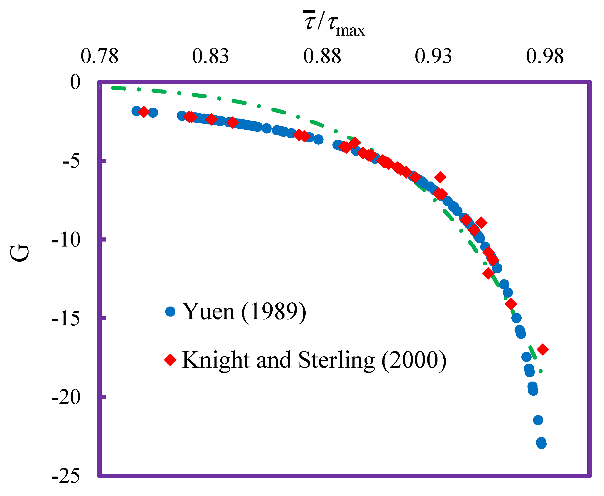
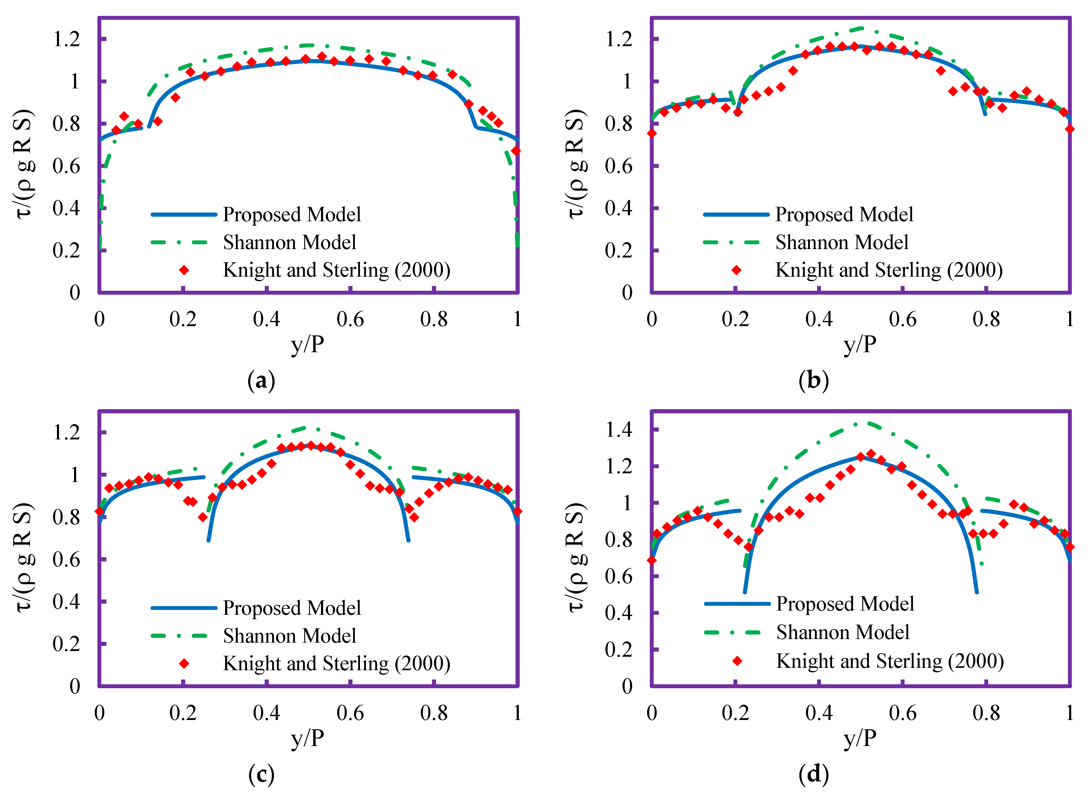
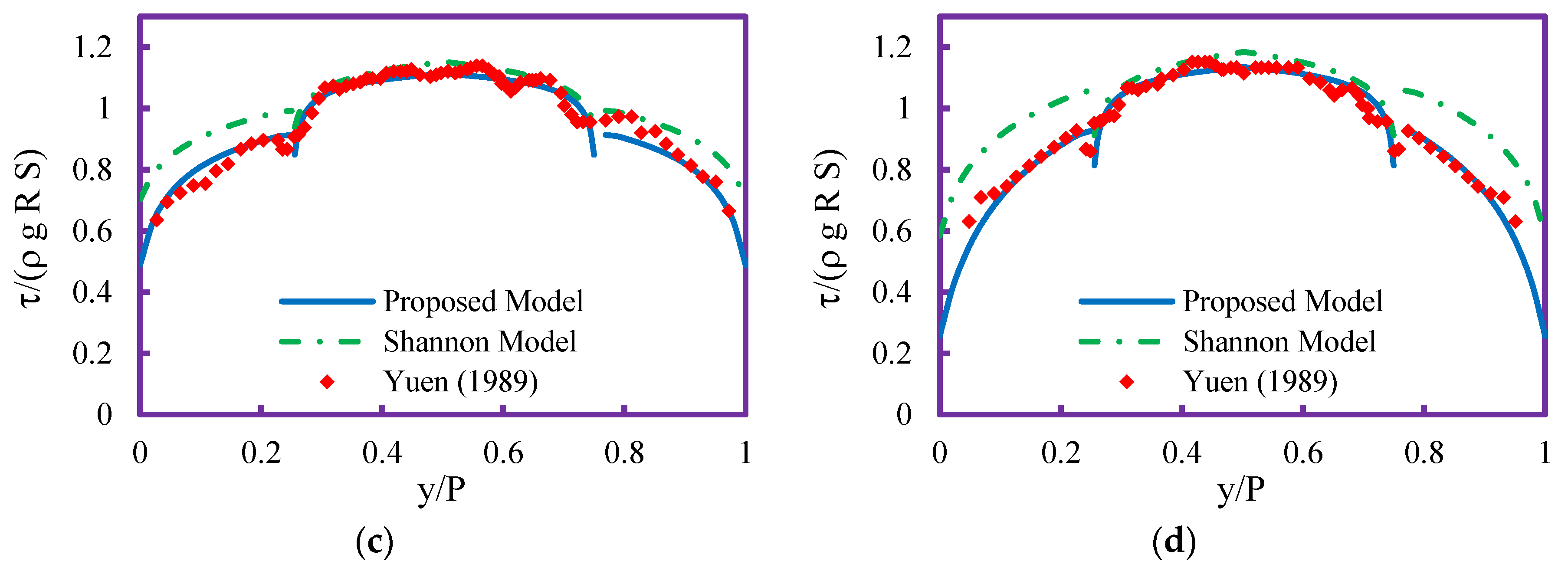
4. Data Used
5. Performance Evaluation
6. Results
7. Conclusions
Author Contributions
Funding
Conflicts of Interest
References
- Knight, D.W.; Demetriou, J.D.; Hamed, M.E. Boundary shear in smooth rectangular channels. J. Hydraul. Eng. 1984, 110, 405–422. [Google Scholar] [CrossRef]
- Seckin, G.; Seckin, N.; Yurtal, R. Boundary shear stress analysis in smooth rectangular channels. Can. J. Civ. Eng. 2006, 33, 336–342. [Google Scholar] [CrossRef]
- Tominaga, A.; Nezu, I.; Ezaki, K.; Nakagawa, H. Three-dimensional turbulent structure in straight open channel flows. J. Hydraul. Res. 1989, 27, 149–173. [Google Scholar] [CrossRef]
- Alhamid, A. Boundary Shear Stress and Velocity Distribution in Differentially Roughened Trapezoidal Open Channels. Ph.D. Thesis, University of Birmingham, Birmingham, UK, 1991. [Google Scholar]
- Yuen, K.W.H. A Study of Boundary Shear Stress Flow Resistance and Momentum Transfer in Open Channels with Simple and Compound Trapezoidal Cross Section. Ph.D. Thesis, University of Birmingham, Birmingham, UK, 1989. [Google Scholar]
- Knight, D.W.; Sterling, M. Boundary shear in circular pipes running partially full. J. Hydraul. Eng. 2000, 126, 263–275. [Google Scholar] [CrossRef]
- Kleijwegt, R.A. On Sediment Transport in Circular Sewers with Non-cohesive Deposits. Ph.D. Thesis, Delft University of Technology, Delft, The Netherlands, 1992. [Google Scholar]
- Khodashenas, S.R.; Paquier, A. A geometrical method for computing the distribution of boundary shear stress across irregular straight open channels. J. Hydraul. Res. 1999, 37, 381–388. [Google Scholar] [CrossRef]
- Yang, S.-Q.; Lim, S.-Y. Boundary shear stress distributions in trapezoidal channels. J. Hydraul. Res. 2005, 43, 98–102. [Google Scholar] [CrossRef]
- Zarrati, A.R.; Jin, Y.C.; Karimpour, S. Semianalytical model for shear stress distribution in simple and compound open channels. J. Hydraul. Eng. 2008, 134, 205–215. [Google Scholar] [CrossRef]
- Sheikh Khozani, Z.; Bonakdari, H.; Ebtehaj, I. An analysis of shear stress distribution in circular channels with sediment deposition based on Gene Expression Programming. Int. J. Sediment Res. 2017, 32, 575–584. [Google Scholar] [CrossRef]
- Sheikh Khozani, Z.; Bonakdari, H.; Zaji, A.H. Estimating shear stress in a rectangular channel with rough boundaries using an optimized SVM method. Neural Comput. Appl. 2018, 30, 1–13. [Google Scholar]
- Sheikh Khozani, Z.; Bonakdari, H. A comparison of five different models in predicting the shear stress distribution in straight compound channels. Sci. Iran. Trans. A Civ. Eng. 2016, 23, 2536–2545. [Google Scholar] [CrossRef][Green Version]
- Afan, H.A.; El-shafie, A.; Mohtar, W.H.M.W.; Yaseen, Z.M. Past, present and prospect of an Artificial Intelligence (AI) based model for sediment transport prediction. J. Hydrol. 2016, 541, 902–913. [Google Scholar] [CrossRef]
- Wan Mohtar, W.H.M.; Afan, H.; El-Shafie, A.; Bong, C.H.J.; Ab. Ghani, A. Influence of bed deposit in the prediction of incipient sediment motion in sewers using artificial neural networks. Urban Water J. 2018, 15, 296–302. [Google Scholar] [CrossRef]
- Uca; Toriman, E.; Jaafar, O.; Maru, R.; Arfan, A.; Ahmar, A.S. Daily Suspended Sediment Discharge Prediction Using Multiple Linear Regression and Artificial Neural Network. J. Phys. Conf. Ser. 2018, 954, 012030. [Google Scholar]
- Sheikh Khozani, Z.; Hosseinjanzadeh, H.; Wan Mohtar, W.H.M. Shear force estimation in rough boundaries using SVR method. Appl. Water Sci. 2019, 9, 186. [Google Scholar] [CrossRef]
- Sheikh Khozani, Z.; Bonakdari, H.; Zaji, A.H. Application of a genetic algorithm in predicting the percentage of shear force carried by walls in smooth rectangular channels. Measurement 2016, 87, 87–98. [Google Scholar] [CrossRef]
- Sheikh Khozani, Z.; Khosravi, K.; Pham, B.T.; Kløve, B.; Wan Mohtar, W.H.M.; Yaseen, Z.M. Determination of compound channel apparent shear stress: application of novel data mining models. J. Hydroinform. 2019, 21, 798–811. [Google Scholar] [CrossRef]
- Sheikh Khozani, Z.; Bonakdari, H.; Ebtehaj, I. An expert system for predicting shear stress distribution in circular open channels using gene expression programming. Water Sci. Eng. 2018, 11, 167–176. [Google Scholar] [CrossRef]
- Sheikh Khozani, Z.; Bonakdari, H.; Zaji, A.H. Estimating the shear stress distribution in circular channels based on the randomized neural network technique. Appl. Soft Comput. 2017, 58, 441–448. [Google Scholar] [CrossRef]
- Chiu, C.L. Entropy and probability concepts in hydraulics. J. Hydraul. Eng. 1987, 113, 583–600. [Google Scholar] [CrossRef]
- Luo, H.; Singh, V.P. Entropy Theory for Two-Dimensional Velocity Distribution. J. Hydrol. Eng. 2011, 16, 303–315. [Google Scholar] [CrossRef]
- Cui, H.; Singh, V.P. Suspended sediment concentration in open channels using Tsallis entropy. J. Hydrol. Eng. 2013, 19, 966–977. [Google Scholar] [CrossRef]
- Sterling, M.; Knight, D. An attempt at using the entropy approach to predict the transverse distribution of boundary shear stress in open channel flow. Stoch. Environ. Res. risk Assess. 2002, 16, 127–142. [Google Scholar] [CrossRef]
- Bonakdari, H.; Sheikh, Z.; Tooshmalani, M. Comparison between Shannon and Tsallis entropies for prediction of shear stress distribution in open channels. Stoch. Environ. Res. Risk Assess. 2015, 29, 1–11. [Google Scholar] [CrossRef]
- Zhang, D.; Jia, X.; Ding, H.; Ye, D.; Thakor, N.V. Application of tsallis entropy to EEG: Quantifying the presence of burst suppression after asphyxial cardiac arrest in rats. IEEE Trans. Biomed. Eng. 2010, 57, 867–874. [Google Scholar] [CrossRef] [PubMed]
- Vila, M.; Bardera, A.; Feixas, M.; Sbert, M. Tsallis mutual information for document classification. Entropy 2011, 13, 1694–1707. [Google Scholar] [CrossRef]
- Varotsos, P.; Sarlis, N.; Skordas, E. Tsallis Entropy Index q and the Complexity Measure of Seismicity in Natural Time under Time Reversal before the M9 Tohoku Earthquake in 2011. Entropy 2018, 20, 757. [Google Scholar] [CrossRef]
- Mirauda, D.; De Vincenzo, A.; Pannone, M. Simplified entropic model for the evaluation of suspended load concentration. Water 2018, 10, 378. [Google Scholar] [CrossRef]
- Sheikh, Z.; Bonakdari, H. Prediction of boundary shear stress in circular and trapezoidal channels with entropy concept. Urban Water J. 2016, 13, 629–636. [Google Scholar] [CrossRef]
- Sheikh Khozani, Z.; Bonakdari, H. Formulating the shear stress distribution in circular open channels based on the Renyi entropy. Phys. A Stat. Mech. Its Appl. 2018, 490, 114–126. [Google Scholar] [CrossRef]
- Zhu, Z.; Yu, J. Estimating the Bed-Load Layer Thickness in Open Channels by Tsallis Entropy. Entropy 2019, 21, 123. [Google Scholar] [CrossRef]
- Bonakdari, H.; Tooshmalani, M.; Sheikh, Z. Predicting shear stress distribution in rectangular channels using entropy concept. Int. J. Eng. Trans. A Basics 2015, 28, 360–367. [Google Scholar]
- Tsallis, C. Possible generalization of Boltzmann-Gibbs statistics. J. Stat. Phys. 1988, 52, 479–487. [Google Scholar] [CrossRef]
- Jaynes, E.T. On the rationale of maximum-entropy methods. Proc. IEEE 1982, 70, 939–952. [Google Scholar] [CrossRef]
- Jaynes, E.T. Information theory and statistical mechanics. II. Phys. Rev. 1957, 106, 620. [Google Scholar] [CrossRef]
- Knight, D.W.; Yuen, K.W.H.; Alhamid, A.A.I. Boundary Shear Stress Distributions in Open Channel Flow in Physical Mechanisms of Mixing and Transport in the Environment; Beven, K., Chatwin, P.C., Millbark, J., Eds.; John Wiley & Sons: Hoboken, NJ, USA, 1994. [Google Scholar]
- Moriasi, D.N.; Arnold, J.G.; Van Liew, M.W.; Binger, R.L.; Harmel, R.D.; Veith, T.L. Model evaluation guidelines for systematic quantification of accuracy in watershed simulations. Trans. ASABE 2007, 50, 885–900. [Google Scholar] [CrossRef]


| Difference | ||||||
|---|---|---|---|---|---|---|
| 1.6350 | 1.8000 | 4.9600 | −10.6850 | 5.0814 | 4.8790 | 0.2024 |
| 0.4752 | 0.5234 | 12.5560 | −7.8562 | 5.0954 | 4.8978 | 0.1976 |
| 0.2242 | 0.2465 | 22.2818 | −6.5571 | 5.1651 | 4.9787 | 0.1864 |
| 3.1000 | 3.4090 | 3.1020 | −12.6280 | 5.1502 | 4.9784 | 0.1718 |
| 0.5824 | 0.6405 | 10.8627 | −8.3102 | 5.1432 | 4.9731 | 0.1701 |
| 0.4249 | 0.4670 | 13.8670 | −7.7230 | 5.1927 | 5.0270 | 0.1657 |
| 1.2230 | 1.0940 | 6.3780 | −9.8240 | 3.8545 | 3.7076 | 0.1469 |
| 0.2943 | 0.3221 | 18.9670 | −7.2327 | 5.4381 | 5.4211 | 0.0170 |
| 0.5216 | 0.5705 | 12.4250 | −8.3823 | 5.4816 | 5.4765 | 0.0051 |
| 0.6246 | 0.6458 | 24.1077 | −16.6096 | 14.9796 | 14.9982 | −0.0186 |
| 0.6360 | 0.6950 | 10.802 | −8.8600 | 5.5503 | 5.5737 | −0.0234 |
| 0.5935 | 0.6468 | 11.6858 | −8.8789 | 5.7238 | 5.8514 | −0.1276 |
| 2.9928 | 3.2610 | 3.4788 | −13.3221 | 5.7361 | 5.8698 | −0.1337 |
| 0.5225 | 0.5675 | 13.3073 | −8.8166 | 5.9733 | 6.2114 | −0.2381 |
| t/D | Case | h(mm) | (h+‘t)/D | S0 | Q (Ls−1) | τ0 (Pa) | Fr |
|---|---|---|---|---|---|---|---|
| 0.25 | 1 | 20.3 | 0.333 | 0.00862 | 3.39 | 1.176 | 0.663 |
| 2 | 36.3 | 0.398 | 0.00196 | 3.30 | 0.5447 | 0.656 | |
| 3 | 60.8 | 0.499 | 0.00196 | 8.00 | 0.8044 | 0.748 | |
| 4 | 101.5 | 0.666 | 0.00196 | 16.50 | 1.0920 | 0.680 | |
| 5 | 60.8 | 0.499 | 0.00862 | 18.20 | 3.538 | 1.70 | |
| 6 | 123.2 | 0.755 | 0.00196 | 22.10 | 1.176 | 0.663 | |
| 0.332 | 7 | 40.7 | 0.499 | 0.009 | 12.00 | 0.967 | 1.960 |
| 8 | 81.5 | 0.666 | 0.002 | 12.20 | 0.967 | 0.685 | |
| 9 | 114.2 | 0.800 | 0.002 | 22.10 | 1.106 | 0.721 | |
| 0.5 | 10 | 39.5 | 0.666 | 0.009 | 8.40 | 2.571 | 1.4 |
| 11 | 60 | 0.750 | 0.009 | 16.00 | 3.340 | 1.42 | |
| 12 | 72.2 | 0.800 | 0.009 | 20.00 | 3.645 | 1.33 |
| Case | Expt. No. | h(m) | b/h | S0 | Q (Ls1) | τ0 (Pa) | Fr |
|---|---|---|---|---|---|---|---|
| 13 | 001 | 0.0300 | 5.000 | 0.001 | 1.3000 | 0.2256 | 0.4794 |
| 14 | 002 | 0.0375 | 4.000 | 0.001 | 4.650 | 0.2693 | 0.5455 |
| 15 | 012 | 0.0938 | 1.599 | 0.001 | 10.60 | 0.5398 | 0.5693 |
| 16 | 018 | 0.0585 | 0.752 | 0.001 | 1.650 | 0.2807 | 0.4553 |
| 17 | 022 | 0.0360 | 12.5 | 0.001 | 5.700 | 0.3109 | 0.5682 |
| 18 | 103 | 0.0440 | 10.23 | 0.001 | 19.40 | 1.4727 | 1.4179 |
| 19 | 208 | 0.0449 | 10.23 | 0.009 | 30.01 | 3.2305 | 2.1934 |
| 20 | 302 | 0.0745 | 2.013 | 0.015 | 32.50 | 6.6020 | 2.6236 |
| 21 | 408 | 0.044 | 1.000 | 0.023 | 6.500 | 5.2680 | 3.1299 |
| 22 | 412 | 0.0445 | 10.11 | 0.023 | 50.00 | 8.7577 | 3.5910 |
| Statistical Parameters | Performance Evaluation Criteria | |||
|---|---|---|---|---|
| Very good | Good | Satisfactory | Unsatisfactory | |
| RSR | 0.00 < RSR < 0.50 | 0.50 < RSR < 0.60 | 0.60 < RSR < 0.70 | RSR > 0.70 |
| PBIAS | PBIAS< ± 10 | ± 10 ≤ PBIAS < ± 15 | ± 15 ≤ PBIAS < ± 25 | PBIAS ≥ ± 25 |
| NSE | NSE> 0.80 | 0.70 < NSE ≤ 0.80 | 0.50 < NSE ≤ 0.70 | NSE ≤ 0.50 |
| RMSE | The lower RMSE value, the better model performance | |||
| MAE | The lower MAE value, the better model performance | |||
| Case No. | Proposed Model | Shannon Model | ||||||||
|---|---|---|---|---|---|---|---|---|---|---|
| RMSE | MAE | RSR | PBIAS | NSE | RMSE | MAE | RSR | PBIAS | NSE | |
| 1 | 0.0544 | 0.0367 | 0.4025 | 0.0147 | 0.8096 | 0.0899 | 0.0645 | 0.6256 | 0.0485 | 0.4796 |
| 3 | 0.0701 | 0.503 | 0.5824 | 0.0330 | 0.6923 | 0.1060 | 0.0675 | 0.8409 | 0.0649 | 0.2965 |
| 7 | 0.0619 | 0.0472 | 0.3842 | −0.0195 | 0.8243 | 0.0824 | 0.0530 | 0.4608 | 0.0153 | 0.6891 |
| 8 | 0.0855 | 0.0563 | 0.5774 | 0.0520 | 0.5954 | 0.1815 | 0.1408 | 0.8627 | 0.1400 | −0.8213 |
| 17 | 0.0347 | 0.0133 | 0.2602 | 0.0121 | 0.9314 | 0.0565 | 0.0297 | 0.4435 | −0.0055 | 0.818 |
| 18 | 0.0077 | 0.0029 | 0.0677 | 0.0003 | 0.9956 | 0.0537 | 0.0413 | 0.6212 | 0.0306 | 0.7842 |
| 19 | 0.0071 | 0.0031 | 0.0490 | −0.0007 | 0.9977 | 0.0459 | 0.0307 | 0.3929 | 0.0266 | 0.9010 |
| 22 | 0.0139 | 0.0059 | 0.0945 | −0.0041 | 0.9911 | 0.0766 | 0.0587 | 0.6532 | 0.0587 | 0.7300 |
© 2019 by the authors. Licensee MDPI, Basel, Switzerland. This article is an open access article distributed under the terms and conditions of the Creative Commons Attribution (CC BY) license (http://creativecommons.org/licenses/by/4.0/).
Share and Cite
Sheikh Khozani, Z.; Wan Mohtar, W.H.M. Investigation of New Tsallis-Based Equation to Predict Shear Stress Distribution in Circular and Trapezoidal Channels. Entropy 2019, 21, 1046. https://doi.org/10.3390/e21111046
Sheikh Khozani Z, Wan Mohtar WHM. Investigation of New Tsallis-Based Equation to Predict Shear Stress Distribution in Circular and Trapezoidal Channels. Entropy. 2019; 21(11):1046. https://doi.org/10.3390/e21111046
Chicago/Turabian StyleSheikh Khozani, Zohreh, and Wan Hanna Melini Wan Mohtar. 2019. "Investigation of New Tsallis-Based Equation to Predict Shear Stress Distribution in Circular and Trapezoidal Channels" Entropy 21, no. 11: 1046. https://doi.org/10.3390/e21111046
APA StyleSheikh Khozani, Z., & Wan Mohtar, W. H. M. (2019). Investigation of New Tsallis-Based Equation to Predict Shear Stress Distribution in Circular and Trapezoidal Channels. Entropy, 21(11), 1046. https://doi.org/10.3390/e21111046