1. Introduction
The wrought aluminum alloy 2024-T351 is an important light structural metal commonly used in aerospace and other weight-critical applications [
1]. A common approach to modeling the low-cycle fatigue (LCF) life of this material and many other metals is the Coffin–Manson relationship [
1,
2]:
This equation is intended to cover the range of life from 1 to about 20,000 reversals, where macroscopic plastic strain is measurable. However, as has been pointed in the literature [
2], Equation (1) is less successful in fitting data in the very low reversal count range of 1 to about 200. The inadequacy of Equation (1) for modeling a representative LCF data set for 2024-T351 is demonstrated below and motivates an alternative LCF modeling approach.
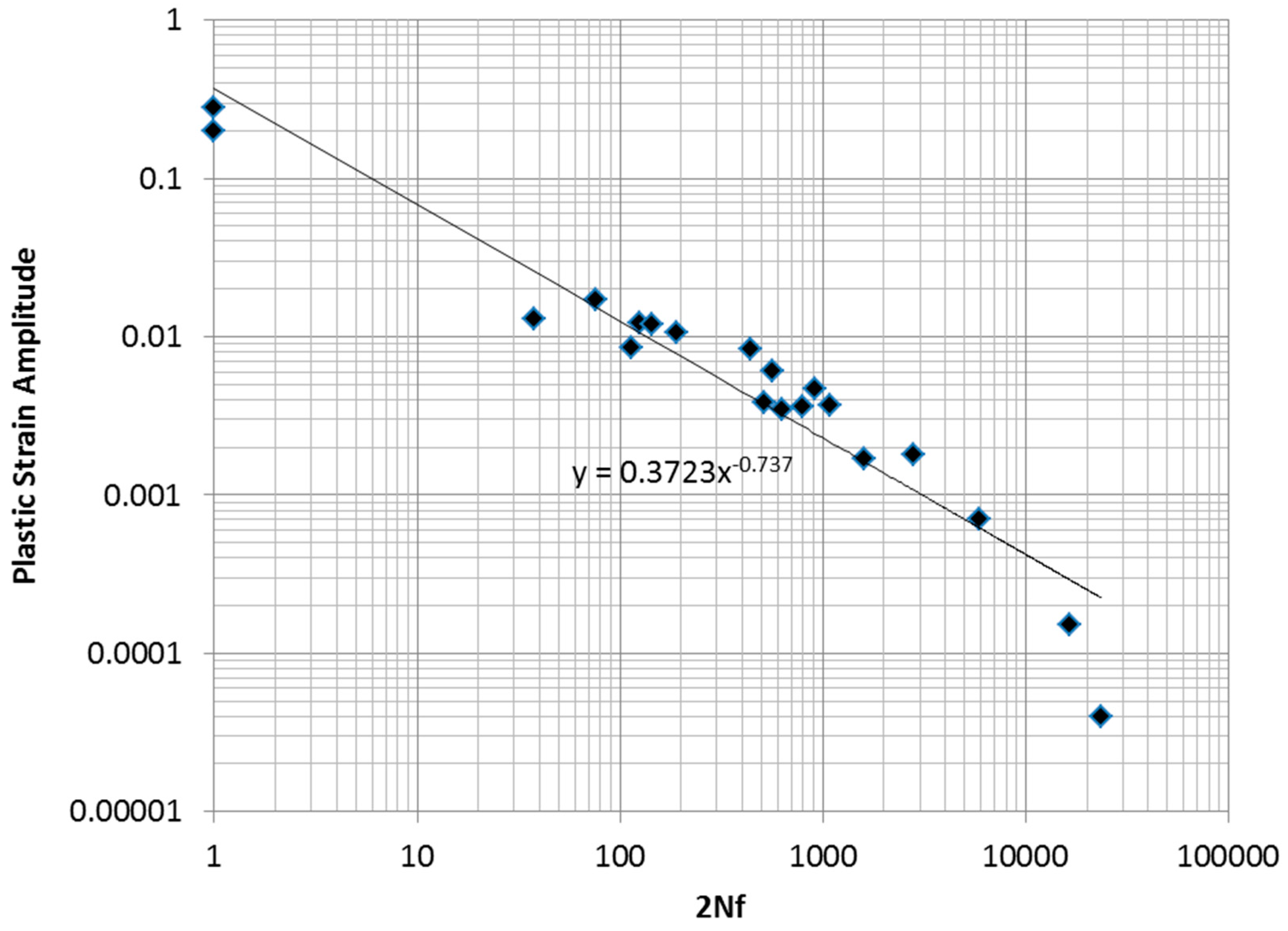
In
Figure 1, the results from a sequence of low-cycle fatigue tests and two monotonic tension tests on tension specimens of 2024-T351 aluminum are shown. The data is also fitted to a Coffin–Manson model in the figure.
It is clear that the data exhibits a curvature that is not captured by the straight line fit of the Coffin–Manson equation. An ideal model would be one based on a sound physical principle that assures the “best possible” fit to experimentally obtained fatigue test data, considering the statistical uncertainty inherent in the data. An ideal procedure would also provide systematic guidance on constructing the model form. Below, we argue that the maximum entropy concept may provide such a guiding principle.
The concept of entropy occurs in two different contexts in the literature reviewed below. The first case is represented by applications of a class of statistical methods based on information entropy (reviewed in detail in the following section), which may be applied to fatigue data or any other experimental data with inherent uncertainty. These applications may not refer to the physical entropy of the material. Alternatively, the physical entropy at a material point in a device or structure may be used to model the progress of damage at that point. In the latter instance, the process of damage and degradation in material behavior is a fundamental consequence of the second law of thermodynamics, resulting in the increase in entropy of isolated systems with time [
3]. In contrast to the more commonly used parameters of stress and plastic strain, the argument is that specimen entropy has a deeper connection to the physics of the damage process.
One of earliest studies to use maximum entropy (or max entropy) probabilistic distributions to study fatigue fracture is [
4]. Entropy as a purely statistical concept is used in [
5] to model the variability of fatigue crack growth. A version of the maximum entropy method is shown to be a viable alternative to Bayesian updating for analyzing an evolving data population. However, the authors do not connect the concept of entropy to material damage. In [
6], the maximum entropy method was used to build a statistical model of the strength distribution in brittle rocks. Since maximum entropy represents a general principle that can lead to many possible probabilistic distributions based on the choice of constraints, studies in the literature have included attempts at specifying constraints on either two or even four moments of the distribution [
4,
7] in an attempt to compute the parameters of the distribution. In general, in [
5,
6,
7], the thermodynamic entropic dissipation at a material point is not directly used to build a predictive fatigue life relationship.
Basaran and co-workers were among the first to make a connection, using the Boltzmann entropy formula, between physical entropy as measured by plastic dissipation and damage in ductile alloys [
8,
9]. Later, Khonsari and co-workers [
10,
11] demonstrated that the thermodynamic entropy generated during a low-cycle fatigue test can serve as a measure of degradation. They proposed that the thermodynamic entropy is a constant when the material reaches its fracture point, independent of geometry, load, and frequency. The hypothesis on critical thermodynamic entropy was tested in [
10] on aluminum 6061-T6 through bending, torsion, and tension–compression fatigue tests. In our prior work [
12], we used the maximum entropy statistical framework to derive a fatigue life model using material entropy as a predictive variable. This approach is inspired by the work of Jaynes [
13], where the information theory concept of entropy was applied to the energy levels of a thermodynamic system, showing that known results from statistical mechanics could be obtained. Information theory entropy was, thus, proportional to thermodynamic entropy. While in some papers [
8,
9] the accumulated damage is empirically related to entropic dissipation, in [
12], the damage
naturally results from the maximum entropy probability distribution as the corresponding cumulative distribution function (CDF). The fatigue life model in [
12] is expressed as a damage function and is given in Equation (2) below. The authors describe this approach as a maximum entropy fracture model.
In Equation (2), the damage parameter
is the non-decreasing CDF that ranges from zero (virgin state) to one (failed state). The independent variable is the inelastic dissipation in the material, which is proportional to the entropy of the material through the J2 plasticity theory and the Clausius–Duhem inequality. The single material parameter
in Equation (2) was obtained from isothermal mechanical cycling tests and then used to model fatigue crack propagation under thermal cycling conditions in an electronic assembly.
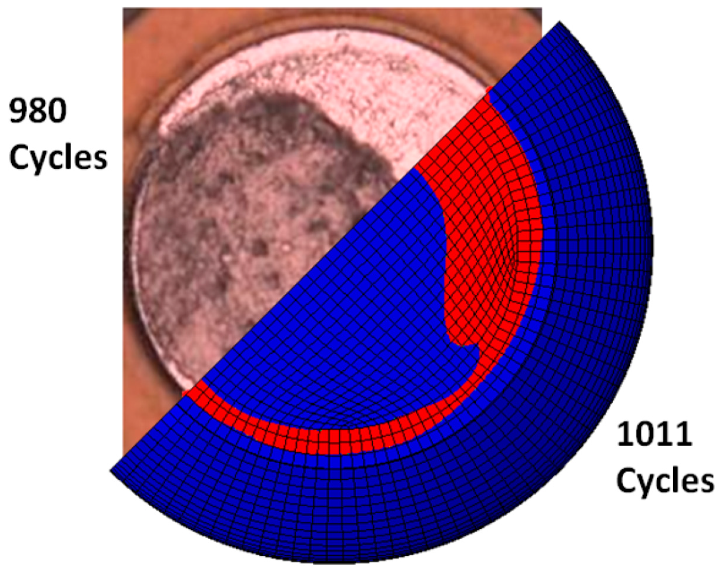
Figure 2 shows a comparison of the estimated and actual number of cycles, as well as crack fronts, at an intermediate stage, with the same area of cracks from both the finite element simulation and thermal cycling fatigue test. To the best of the authors’ knowledge, such a connection between physical entropy dissipation and fatigue crack propagation in ductile alloys has not been made in prior literature.
In [
12], it is demonstrated that it is possible to follow the physical process of fatigue crack propagation as a maximum entropy process. However, the arguments that led to the formation of Equation (2) assumed a constant dissipation rate, which in turn implies an exponential distribution for the form of the statistical distribution. More generally, while the use of maximum entropy principles provides the theoretical advantage of being maximally “non-committal” on the data that are unavailable from the experiments [
13], the assumption of exponential distribution may be restrictive. Arguably, other distributions that conform to the max entropy principle may provide a better description of damage. However, systematic exploration of such maximum entropy functions, as well as thermodynamic entropy, in describing metal fatigue life data sets appears to be limited in the literature. Thus, in this paper, building on our prior work, we propose the development of a systematic procedure for development of maximum entropy models for describing metal fatigue based on measured thermodyanamic entropy. We demonstrate the approach using low-cycle fatigue experimental data for aluminum 2024-T351 material, and generalize the application of the maximum entropy principle using a broader class of statistical distributions, including the truncated exponential and the truncated normal distribution. We begin first with a brief review of the maximum entropy principle.
2. A Review of the Maximum Entropy Principle
The concept of entropy as applied to heat engines is due to Clausius, but the connection of entropy to the probability of the states of a thermodynamic system began with Boltzmann. Boltzmann demonstrated that the second law of thermodynamics for an ideal gas is a consequence of the mechanics of the collisions of the molecules [
14]. He showed that a sufficiently large number of interrelated deterministic events will result in random states. He derived the following function, given in Equation (3), for a uniform distribution, and argued that this quantity had the same physical meaning as the entropy proposed by Clausius. This led to the Boltzmann H function:
The above expression is closely related to Gibb’s entropy formula:
Shannon’s research in information theory led to a mathematical expression (discussed later in Equation (6)) that is strikingly similar to the thermodynamic entropy formulas of Boltzmann and Gibbs, described above. It is important to note that Shannon’s argument was a purely statistical one and no physical significance was claimed. It was not until the work of Jaynes [
13] that a connection between the information entropy of Shannon and thermodynamic entropy was established.
Here, we describe the abstract development of Shannon’s formula based on a counting argument [
15], considering the information content of a whole number, which can range in value from
to
. If we claim that each digit of the number is a unit of information, then it clearly takes
digits to represent the number in a base
system. If the base of the logarithm is changed, the resulting information will change by a constant, but the ratios of information for different
will be preserved, provided the same base is used for all of them. Thus,
is a reasonable measure of the information contained in a variable, which can range from
to
. If we consider a random experiment with
possible equally likely, mutually exclusive outcomes, then the information contained in a given outcome is still
, with
being the probability of the event. We argue that the information in a given event is strictly determined by
, regardless of how the remaining
probability is allocated to other events. Thus, even if the events do not have equal probabilities, the information for any given event is still
[
15]. This function has the expected property that the information contained in the occurrence of two (or more) statistically independent events is the sum of the information in each of the events separately, as shown below in Equation (5). This property is fundamentally important (as pointed out in [
13]) and further reinforces the argument for the
measure of information.
If the events correspond to a discrete random variable, then they must be mutually exclusive, and the probability of the union of the sequence of the events is equal to one [
16]. The entropy of the density function is taken as the expected value of the information in the events [
17]. This leads to the Shannon information entropy formula:
This function (and only this function) satisfies these three conditions:
Continuity: It is a continuous function of the ;
Monotonicity: It is an increasing function of n, if all the are equal;
Composition: If an event can be decomposed into two or more lower level events, the function will evaluate this identically, whether the lower or higher level events are used in the computation, provided that the appropriate conditional probabilities are used to relate the higher and lower level events.
Jaynes [
13] noted that there is a symbolic similarity between the expressions for thermodynamic (Gibbs) entropy (Equation (3)) and Shannon’s information entropy (Equation (6)), but commented that the similarity did not necessarily imply a deeper connection. Jaynes then proceeded to show that a connection did exist and that many results of statistical thermodynamics could be interpreted as applications of Shannon’s information entropy concept to physical systems. The expression for the Gibbs entropy is the result of a development involving various physical assumptions—some based on experimental evidence, and some not. Conversely, Shannon’s entropy is based on mathematical and logical reasoning, not physical evidence. Shannon’s model was developed to model the abstract mathematical properties of digital communication, and prior to Jaynes, was not claimed to be applicable to the physical sciences. Shannon defined the entropy of a discrete probability distribution as Equation (6).
The maximum entropy method as set forth by Jaynes is as follows [
13]: The probability mass function that maximizes Equation (6), subject to constraint from Equations (7) and (8), is the best choice if no other information is available to specify the probability distribution.
where
is the expected value of,
. The following probability mass function (Equation (9)) can be shown to maximize Equation (6):
The constants
and
are Lagrange multipliers associated with the constraints. Jaynes calls this approach the maximum entropy method and calls the derived probability functions maximum entropy distributions (MaxEnt method and MaxEnt distributions). Multiple expected value constraints may be applied (not simply moments, as is common in probability analysis), resulting in the following form of the MaxEnt distribution:
The entropy of the resulting distribution is [
13]:
Jaynes’s argument was for the discrete case. The entropy of a continuous probability density function is also known and is defined as [
16]:
The corresponding continuous version of Equation (10) is given below [
16]:
One important point regarding Equation (13) is that it is only a probability density function for specific values of the parameters . This situation differs from the usual approach to representing probability density functions or distribution functions, where the functions are admissible for ranges of parameter values. Additionally, the method Jaynes sets forth assumes that the values used for moment function constraints are not estimates subject to sampling variation. They are taken as essentially exact values of the distribution moment functions. This assumption differs from traditional inferential statistics, where moments or quantiles are estimated from data and sampling errors are estimated.
Jaynes showed that if we choose the probability distribution for the system microstates based on maximizing Shannon entropy, known results from statistical mechanics can be obtained, without new physical assumptions, and in particular, the thermodynamic entropy of the system is found to be the Gibbs entropy of Equation (4). Shannon’s entropy for the distribution is proportional to the physical entropy of the system, however, only if the probability distribution is applied to the thermodynamic states of the system. Jaynes [
13] argues that this shows that thermodynamic entropy is an application of a more general principle. Further to this point, Jaynes argues that if a probability model is required for some application, where certain expected values are known but other details are not, the maximum entropy approach should be used to find the probability distribution. Jaynes uses the term “maximally non-committal” to describe probability distributions obtained by this process. What is known about the random variable in question is captured in mathematical constraints, while the principle of maximum entropy accounts for what is not known. While information entropy is only proportional to thermodynamic entropy in certain circumstances, Jaynes argues that choosing the probability density function that maximizes the Shannon entropy subject to various constraints is appropriate to any situation where a reference probability distribution is needed. The application could be physical or not, and need not necessarily have a relationship to thermodynamic states.
3. Maximum Entropy Distributions
We argue that if a given parametric family of distributions is selected for some reason (as is common practice), then within that family of distributions we should prefer the parameter values that maximize entropy (subject to any constraints) over those that do not. For example, if the Weibull distribution has already been chosen for some application, and the characteristic life is known, then the Weibull exponent should be chosen to maximize entropy. It is noteworthy that the exponential distribution and the normal distribution are the MaxEnt distributions corresponding to a prescribed mean value and to the prescribed mean and variance values, respectively [
18]. Given the fundamental importance of these distributions in statistical theory, it is informative that they can be directly derived from the principles of maximum entropy. Just as Jaynes showed that statistical thermodynamic results derivable by other means could be obtained from maximum entropy methods, it has also been shown that the well-known and fundamental normal distribution, traditionally derived by other means, can also be based on a maximum entropy argument. Even the Weibull distribution can be derived from a maximum entropy approach if appropriate moment functions are chosen [
18]. These MaxEnt distributions are listed in
Table 1.
Note the references to truncated distributions in
Table 1. A distribution is described as truncated if the value of its density or mass function is forced to zero (when otherwise it would be non-zero) outside of a specific range. Thus, the truncated normal distribution functions can be thought of as ordinary normal probability density functions (PDFs) that are clipped to zero probability outside of their non-zero range. As described later, they are multiplied by a normalizing constant to correct for the missing density. Truncation at
is necessary for applications to non-negative variables. The cumulative distribution function (CDF) of a truncated normal random variable has a finite slope at
. If a second truncation at
is specified, then the CDF is forced to be exactly equal to 1 for all
. We begin the discussion of MaxEnt distributions with the truncated exponential distribution.
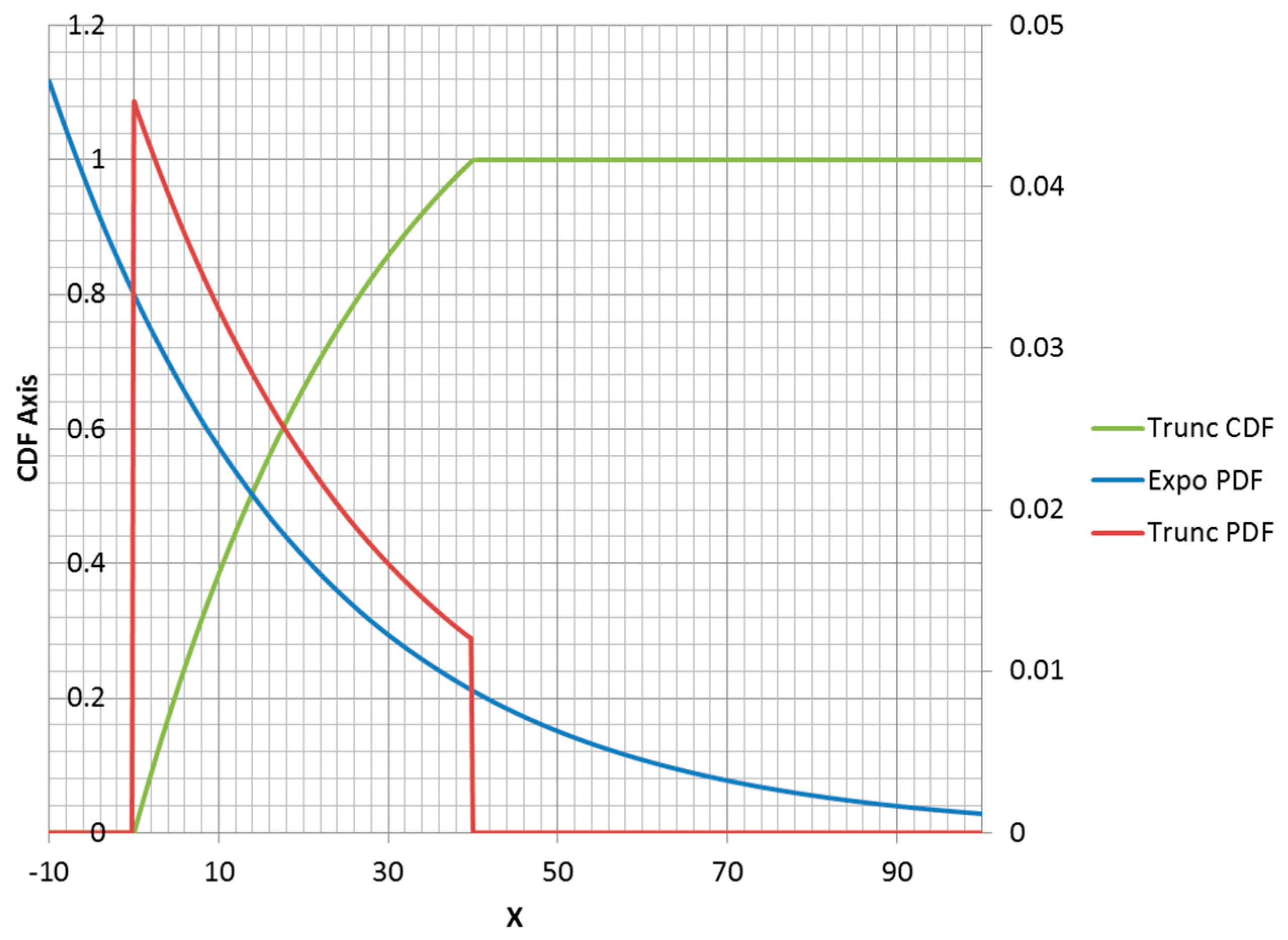
3.1. MaxEnt Form of Truncated Exponential Distribution
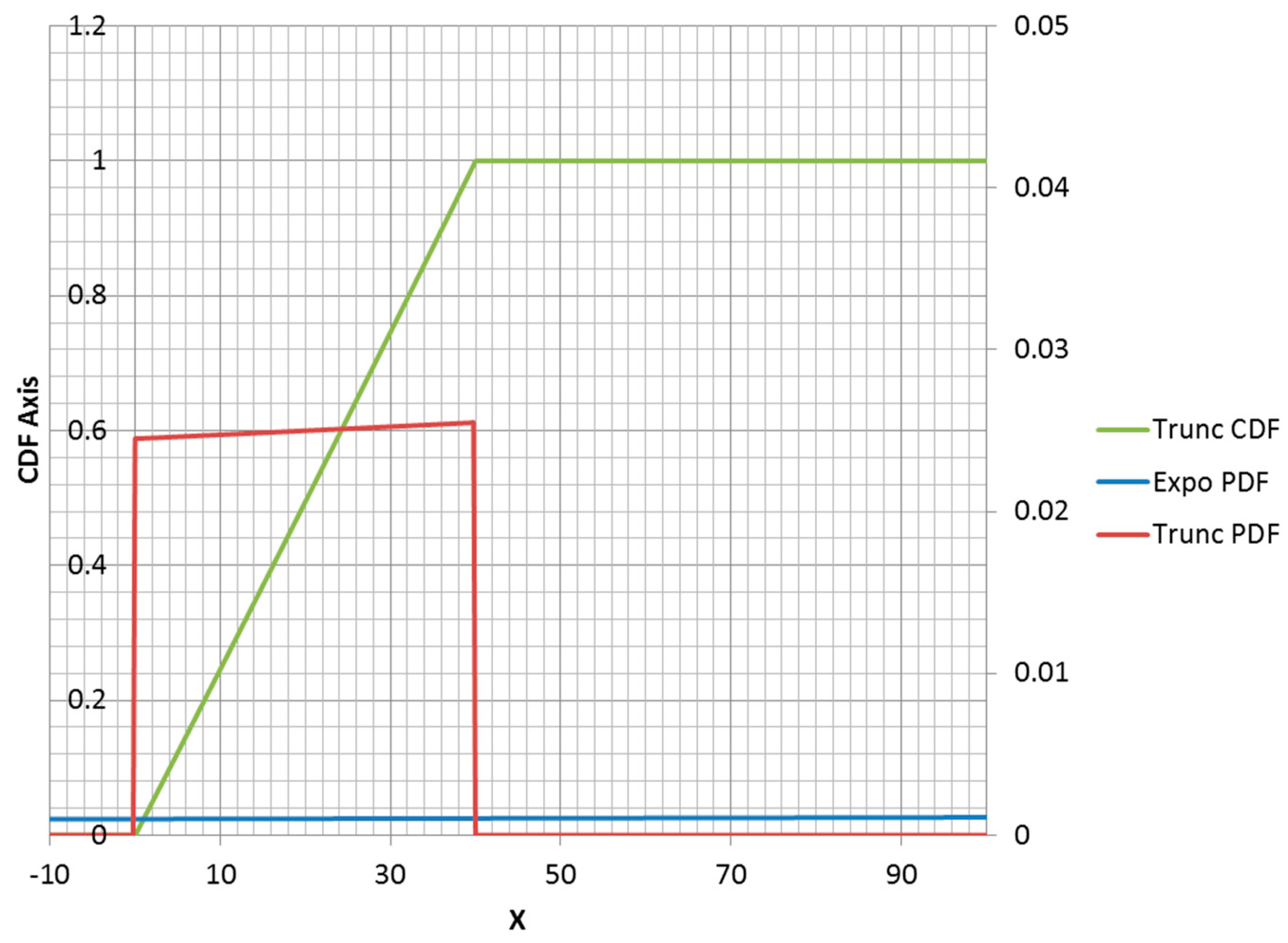
The truncated exponential distribution can be constructed in an analogous fashion for positive values of
(parent PDF is a decreasing function). An example is plotted in
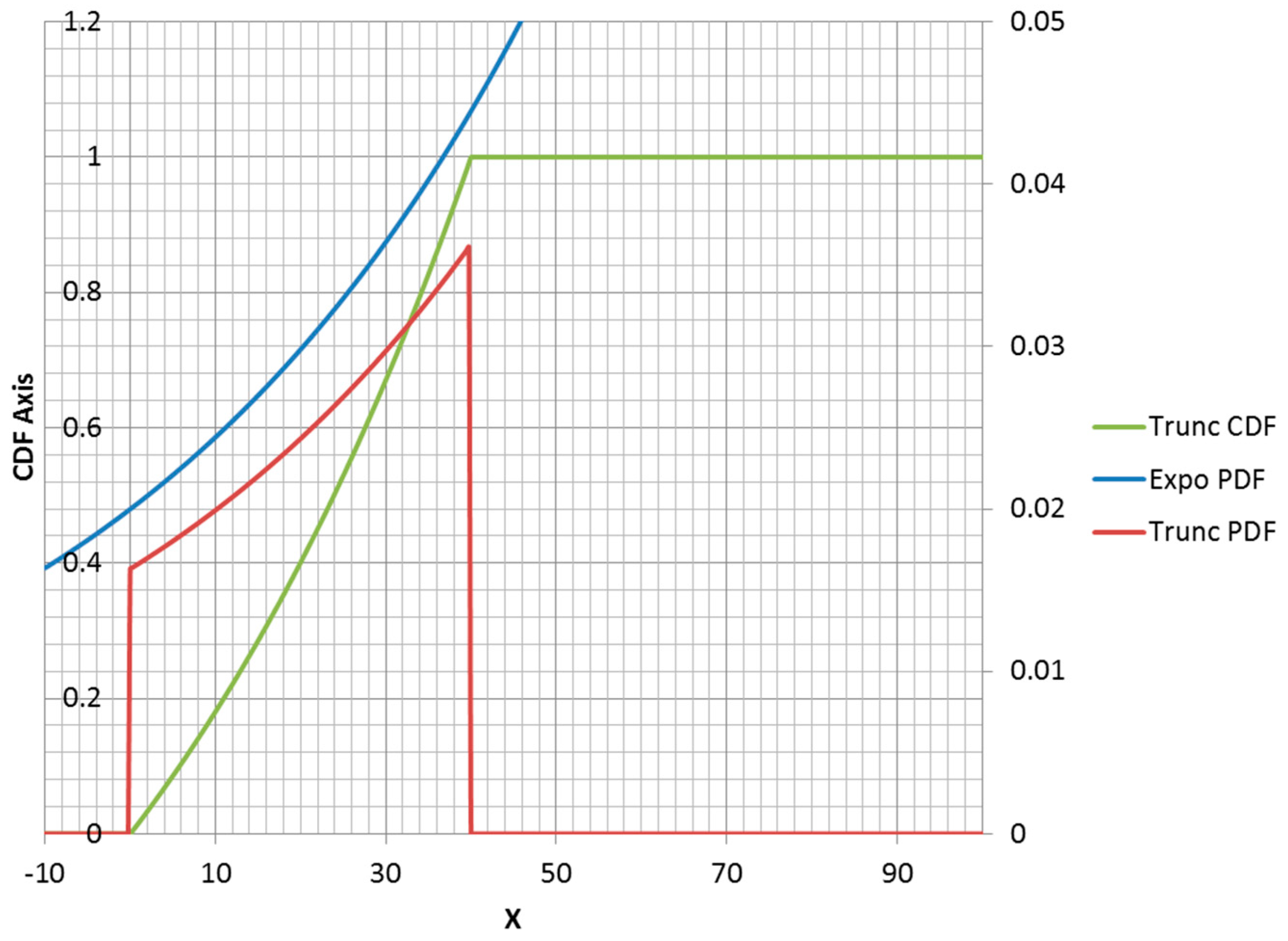
Figure 3. However, it is possible for a truncated exponential distribution to be an increasing function within its non-zero range (
Figure 4). Clipping the positive exponent at some specified value enables its use as a PDF. This corresponds to a negative-valued lambda, which is not admissible in the non-truncated case. If the specified mean was to the right of the midpoint of the non-zero range, then the lambda would be negative.
It should also be noted that changing the location of a distribution function without changing its shape has no effect on the entropy value. Thus, a left endpoint other than zero could be used for any of the distributions that have zero value for negative . Naturally, this shift would change the moment function values. Note that specifying a right truncation value changes the shape of the remaining distribution function and should be thought of as adding an extra parameter. Thus, a truncated exponential distribution is a two-parameter distribution.
Below is the truncated exponential distribution for PDF and CDF:
Below is the expected value of a truncated exponential random variable:
Note that the uniform distribution is a limiting case of the truncated exponential distribution and corresponds to the lambda approaching zero. An example is shown in
Figure 5.
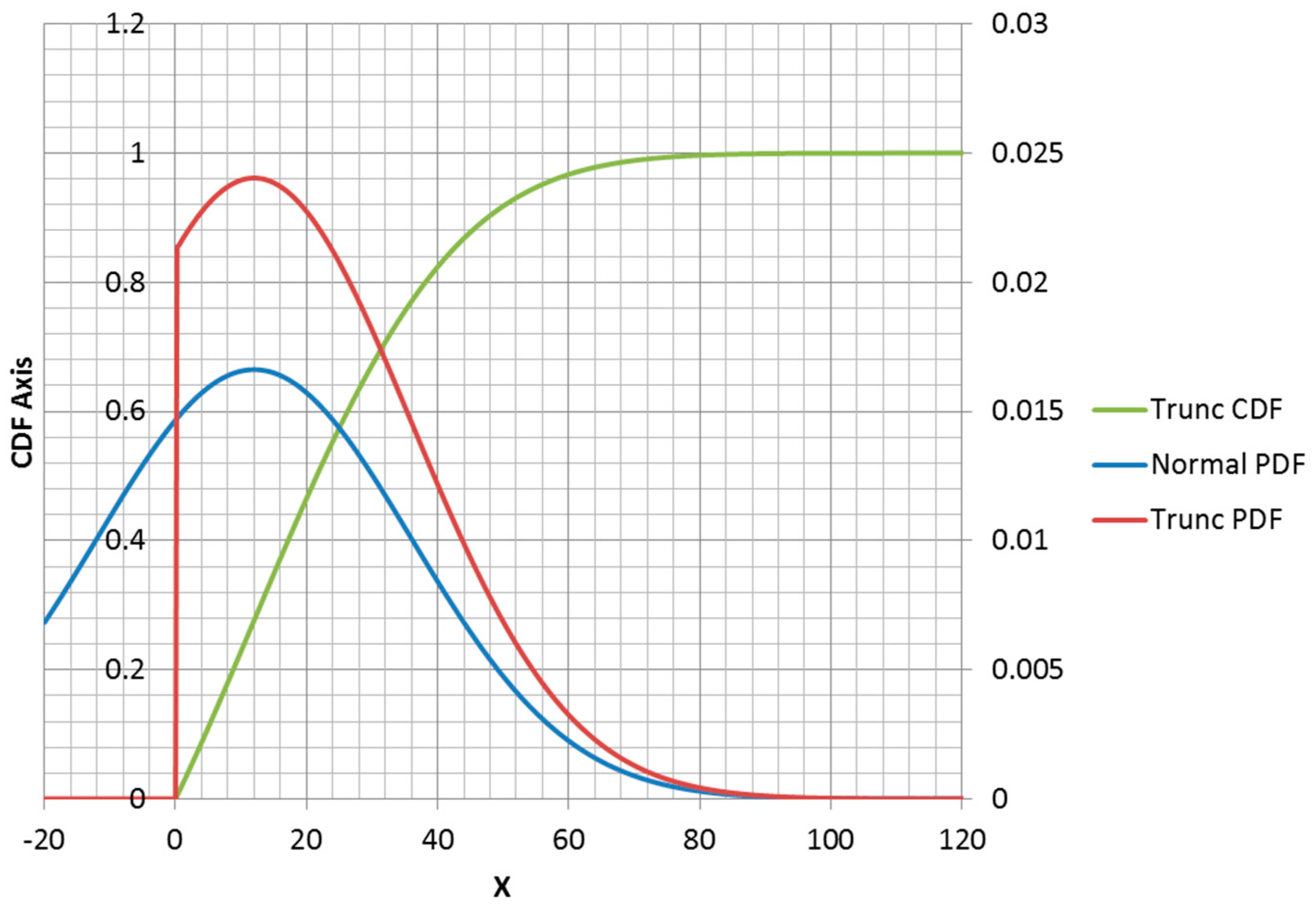
3.2. MaxEnt Form of Truncated Normal Distribution
The truncated normal distribution can be explained in terms of the normal PDF. For
, the PDF has the same shape as a non-truncated normal PDF, but scaled to make up the density lost for
(
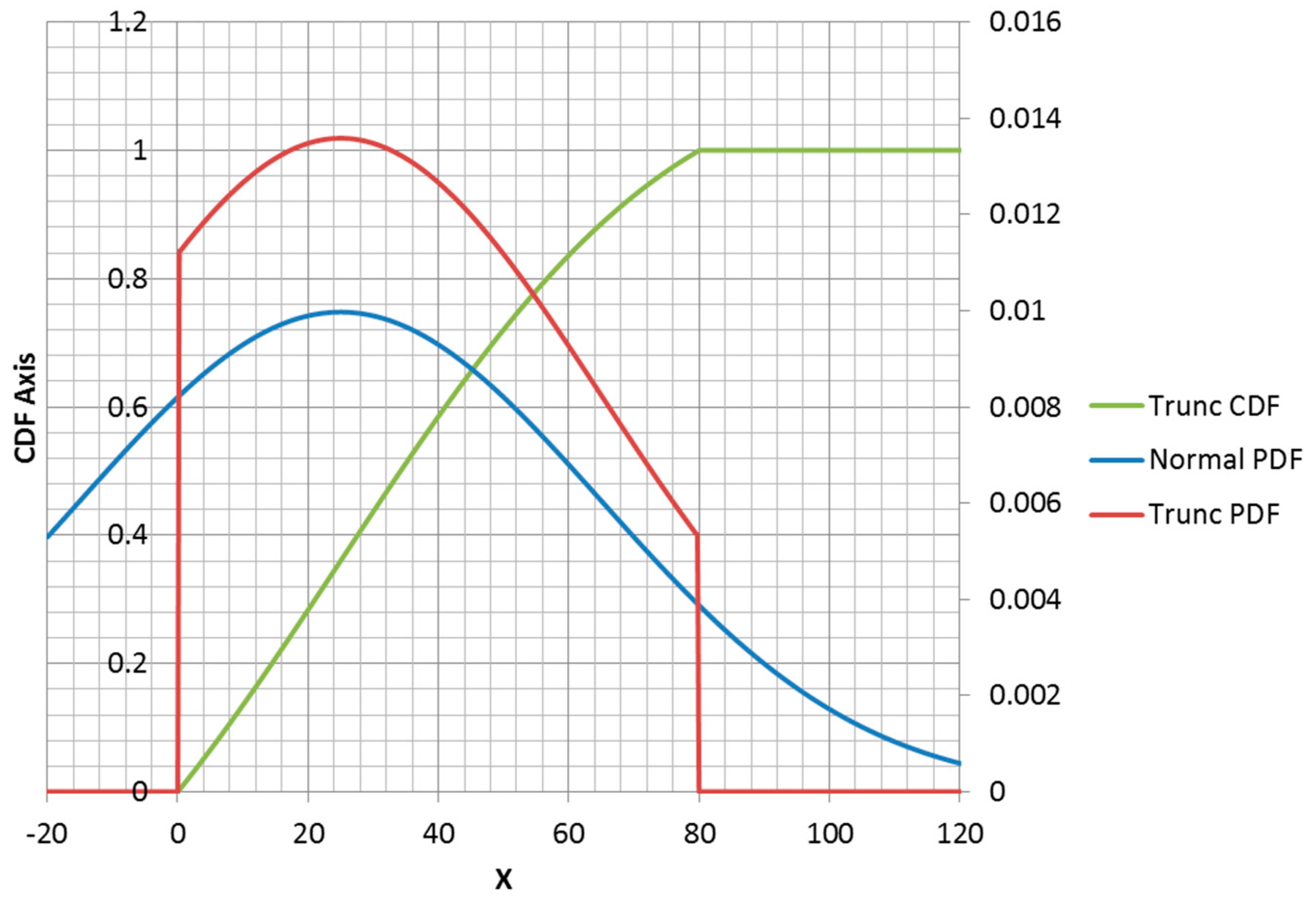
Figure 6). The truncation of the portion of the density less than zero changes the mean and standard deviation from the parameters that the truncated distribution inherits from the normal distribution. Adding a second truncation point at
forces the function to be equal to 1 for all
and adds a corner to the CDF at
(
Figure 7). Additionally, the correction factor must be larger to correct for missing density
and also
.
The PDF and the CDF for the left truncated normal distribution can be shown to be:
The factor in the denominator of the CDF definition in Equation (17) is the area correction factor
.
Truncated normal distribution in two-parameter MaxEnt form is:
Thus, just as the normal distribution is MaxEnt for moment functions x, x2, where x ranges over , the truncated Normal distribution is MaxEnt for the same moment functions over the range . Note that the and are the mean and standard deviation of the parent (un-truncated) normal distribution, not the truncated normal distribution.
3.3. MaxEnt Form of the Weibull Distribution
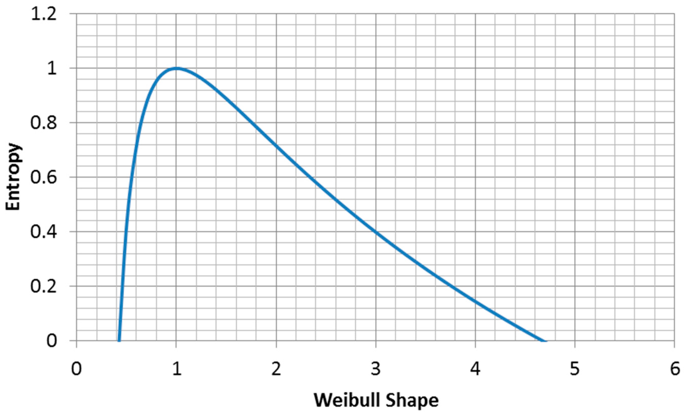
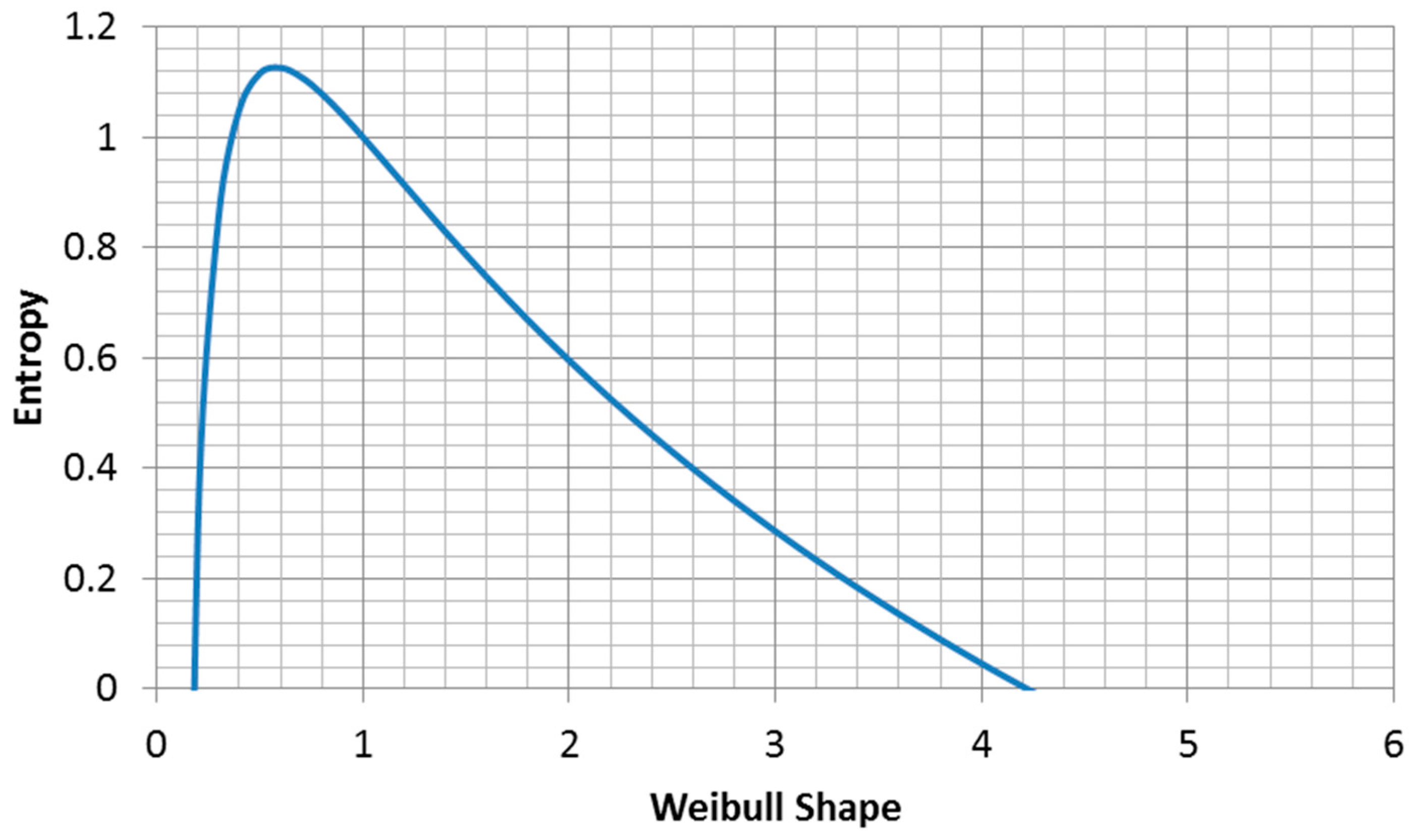
Since the Weibull distribution is widely used, it is useful to know what parameter value choices maximize the entropy of the function. It is often the case that only one of the two parameters is known and we seek a rational approach to assigning a value to the second parameter. In this case, we suggest that choosing the parameter value that maximizes the entropy of the distribution is the correct approach.
The entropy of the Weibull distribution is (
Figure 8, derived from Equation (2.80c) in [
21]):
The mean of a Weibull distribution is [
21]:
Thus, the entropy for a Weibull distribution with a fixed mean (moment constraint on
x) is:
Here, we maximize the entropy function:
Then, we recall the properties of the digamma function [
21]:
This is only true for . Thus, within the Weibull family of distributions, for a given fixed mean, the exponential distribution has the highest entropy, in agreement with Jaynes’s result.
The maximum entropy for fixed characteristic life is (
Figure 9):
Thus, for the fixed characteristic life case, (the Euler’s constant).
4. Application of Maximum Entropy to Low-Cycle Fatigue of 2024-T351 Aluminum
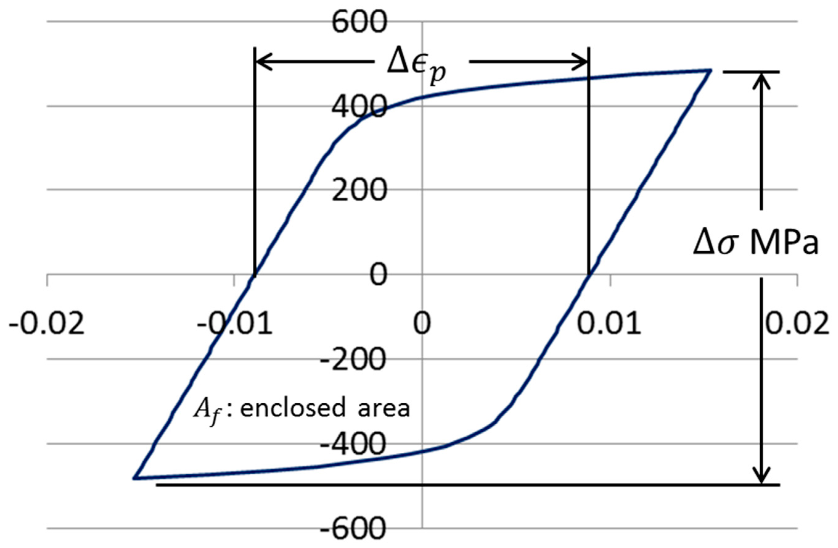
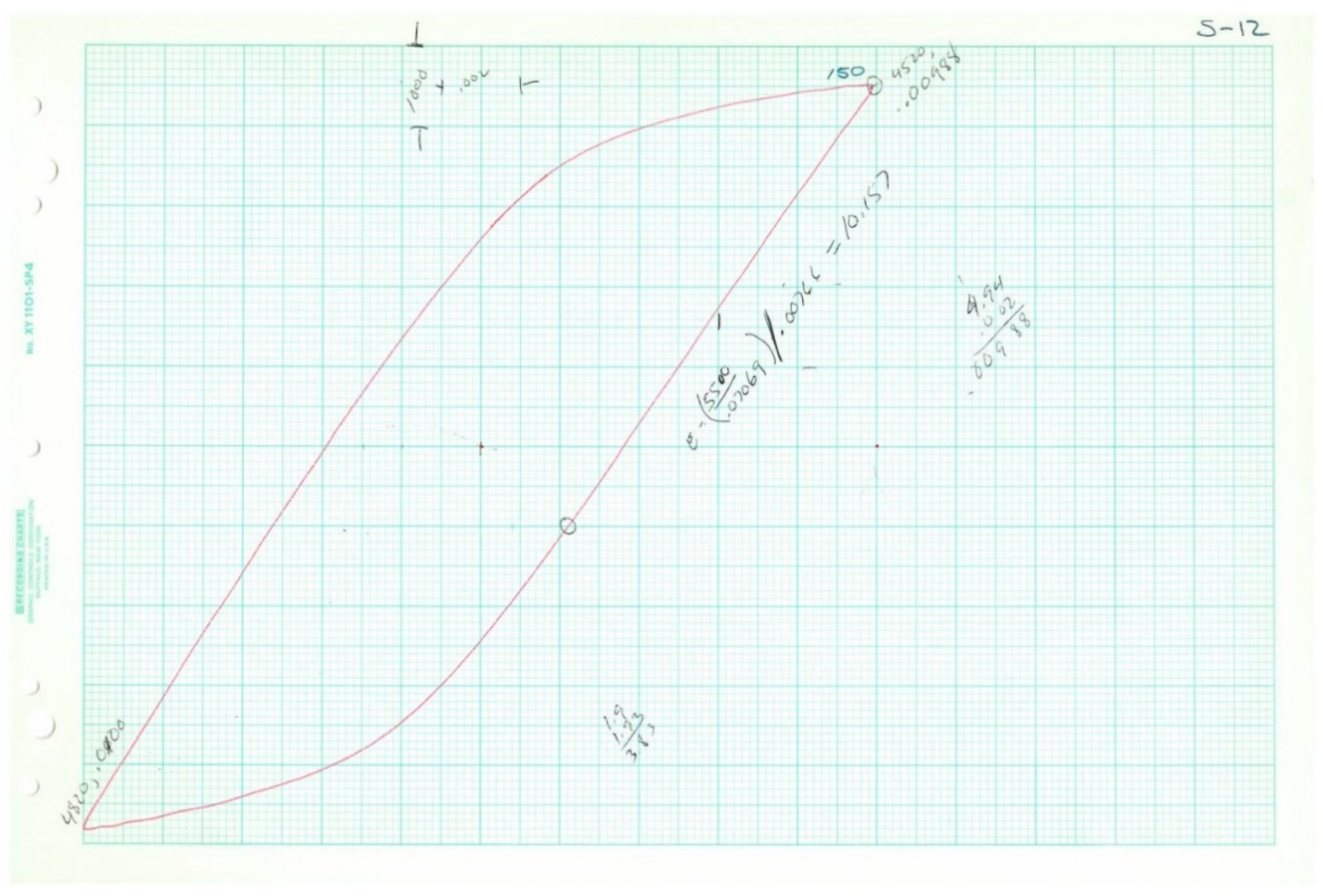
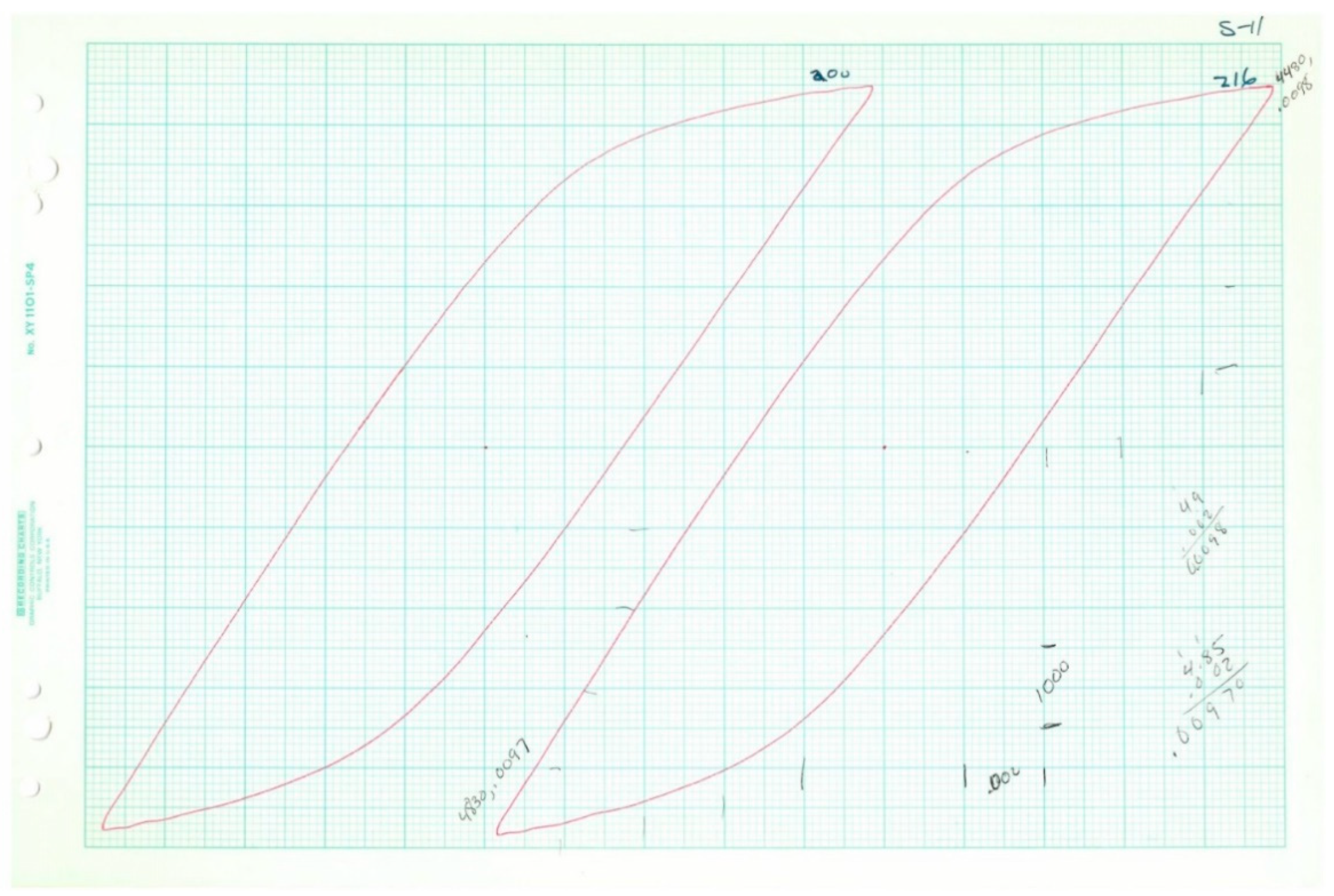
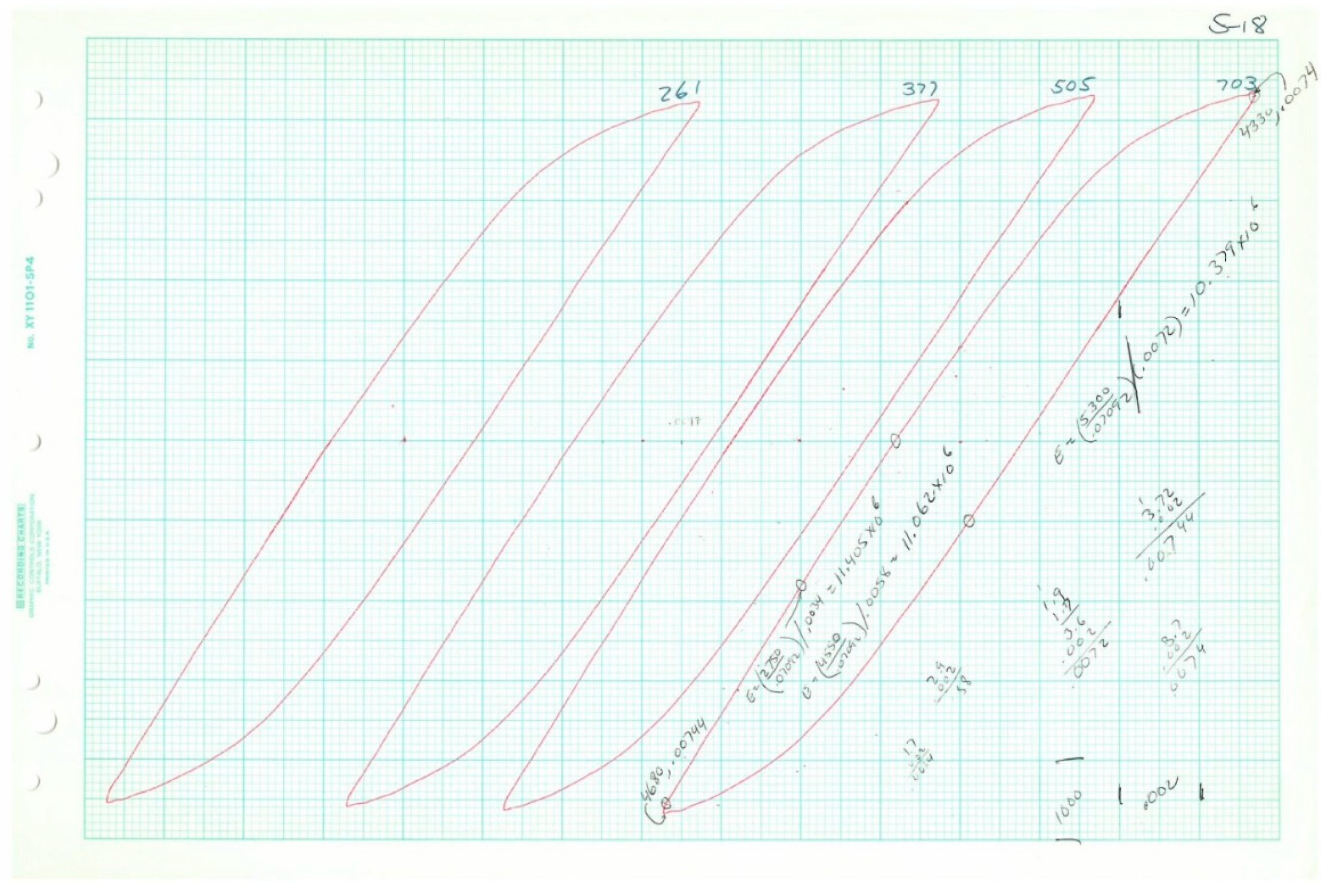
When a specimen is subjected to axial load cycles of a magnitude sufficient to cause plastic deformation, the stress–strain history for the specimen can frequently be described as a loop, as shown in
Figure 10. To determine the fatigue life of the specimen, the load cycles are applied until the specimen fails, or until its compliance exceeds some proportion of its initial compliance. The Coffin–Manson relationship (Equation (1)) is commonly used to model the relationship between plastic strain range and reversals to failure. The parameter
is determined by fitting the curve to fatigue data. It is frequently close in value to
.
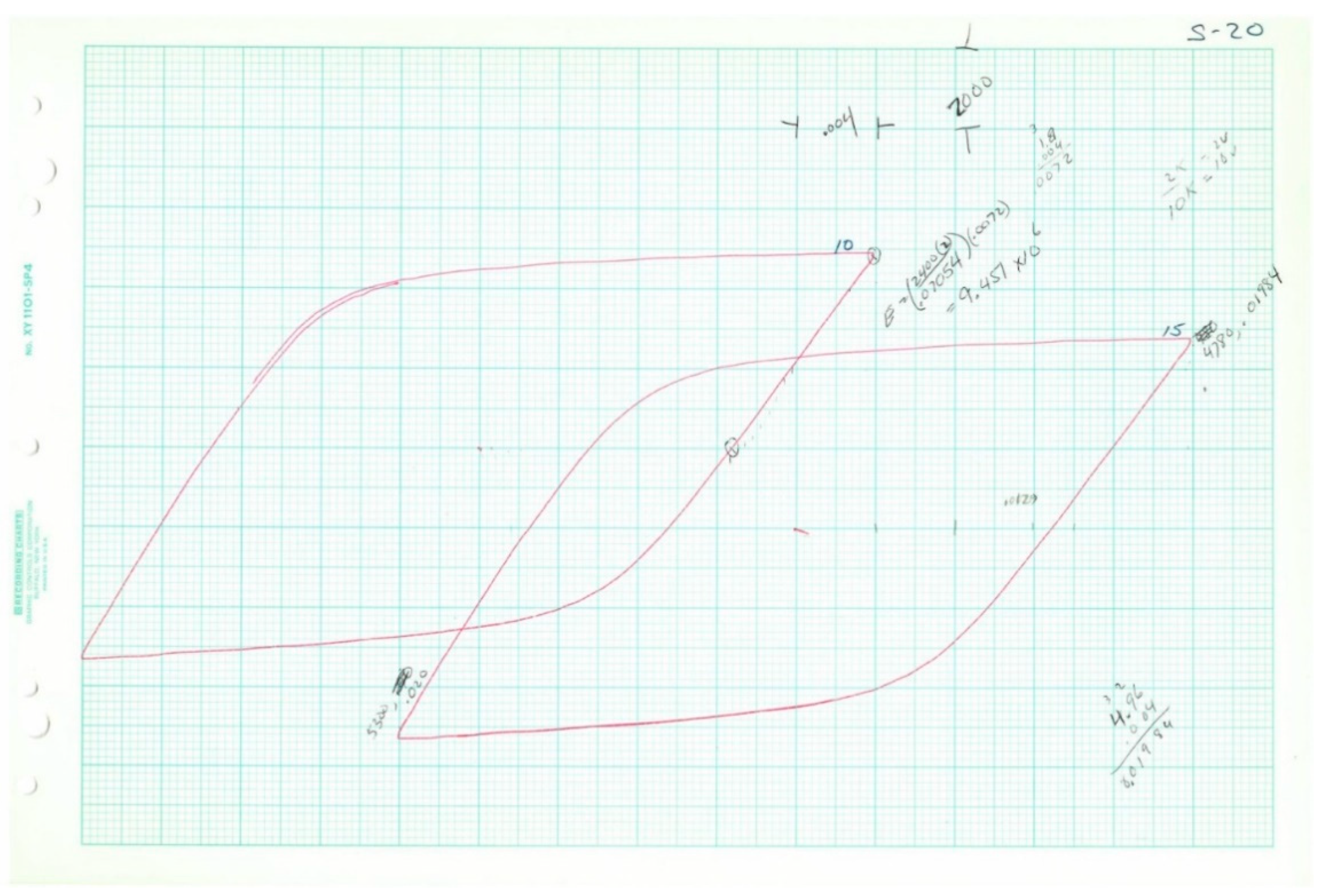
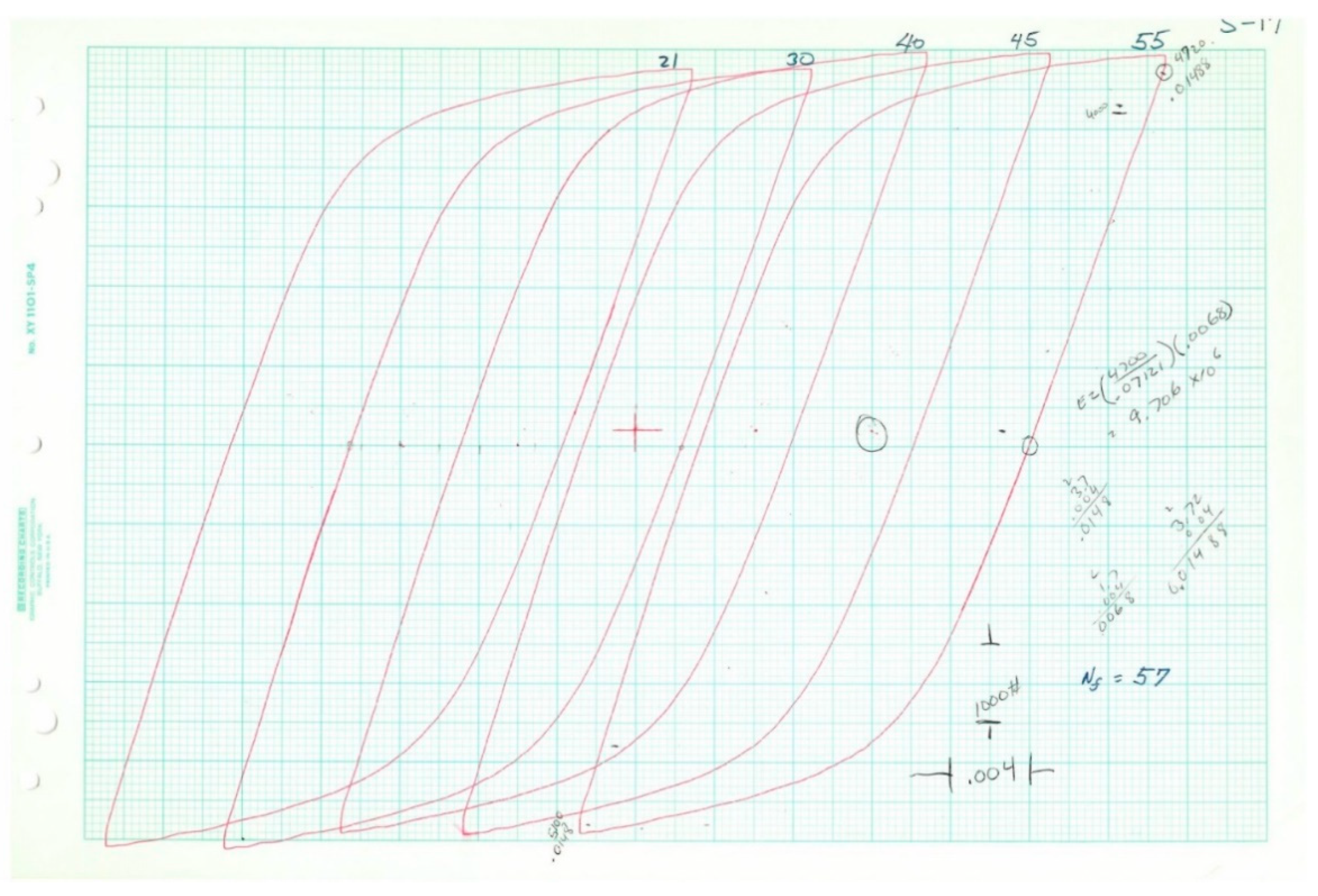
As mentioned earlier, a sequence of low-cycle fatigue tests, along with two monotonic tension tests, was performed on tension specimens of 2024-T351 aluminum. Eighteen specimens were tested under constant-amplitude, fully reversed fatigue conditions. In five cases, representative stress–strain loops were collected at various cycle intervals. Two specimens were tested to failure monotonically. The data collected is summarized in
Table 2. The data is fitted to a Coffin–Manson model, as shown in
Figure 1.
As mentioned earlier, the data exhibits a curvature that is not captured by the straight line fit of the Coffin–Manson power law. An alternative approach to modeling data such as this, using concepts developed from maximum entropy, is developed below. The authors of [
12] showed that material entropy is proportional to inelastic dissipation in experiments such as this, where the temperature of the specimens is essentially constant. Thus, inelastic dissipation is exploited as a surrogate for entropy in the development that follows.
The variable
representing the ability of the material at a point to bear load is fundamental in the literature of damage mechanics [
23]. The value of
(undamaged) represents virgin material, while
is taken to correspond to failed material. The variable
is a non-decreasing quantity, since damage is inherently irreversible. The Coffin–Manson equation can be rewritten in terms of damage, and doing so will be shown to provide a departure point for further development. We begin by rearranging Equation (1) into the following form:
Depending on the application, the damage variable
may be expressed as a function of various independent variables. In fatigue applications, it is common to use the following (applicable to constant damage per load cycle) Palmgren–Miner definition of damage. It is understood that
may depend on other variables, such as temperature or plastic strain amplitude.
We can write the damage accumulation per reversal:
Finally, Equation (28) can be recast as a damage equation as follows:
where
denotes a functional relationship with the argument. Following [
12], we propose developing a function of the form of Equation (31), in terms of energy per reversal rather than plastic strain range. This relationship will have the form:
In the development that follows, a general approach to deriving functions of the form of the above equation will be proposed. In order to apply an equation of the above form to the data in
Table 3, we first need to determine the inelastic dissipation per reversal corresponding to each of the test conditions of the form shown in
Figure 10. The energy expended in inelastic dissipation for a cyclic test under constant conditions is given by the area enclosed by the loop. Note that in
Table 3, actual loop data was only available for five of the 20 tests. In all cases, the plastic strain range and stress range (and reversals to failure) were collected. Fortunately, the shapes of the loops follow known trends, and thus it was possible to deduce the inelastic dissipation for the tests where loops were not available for measurement. The inelastic dissipation for the two monotonic tests was also deduced from the available loop data, although a different analytical approach was used.
The Ramberg–Osgood relationship (Equation (33)) is frequently successful for modeling data such as this. This model assumes that the plastic portion of the strain range is a power law of the stress range. There is no explicit yield point with this model. The total strain range is given by Equation (34) and is used to model the shapes of the loops. For the purposes of fitting Equation (34), the origin of the stress and strain range variables is placed at the lower left corner of the loop.
The Ramberg–Osgood plasticity model for stress–strain loops is [
23]:
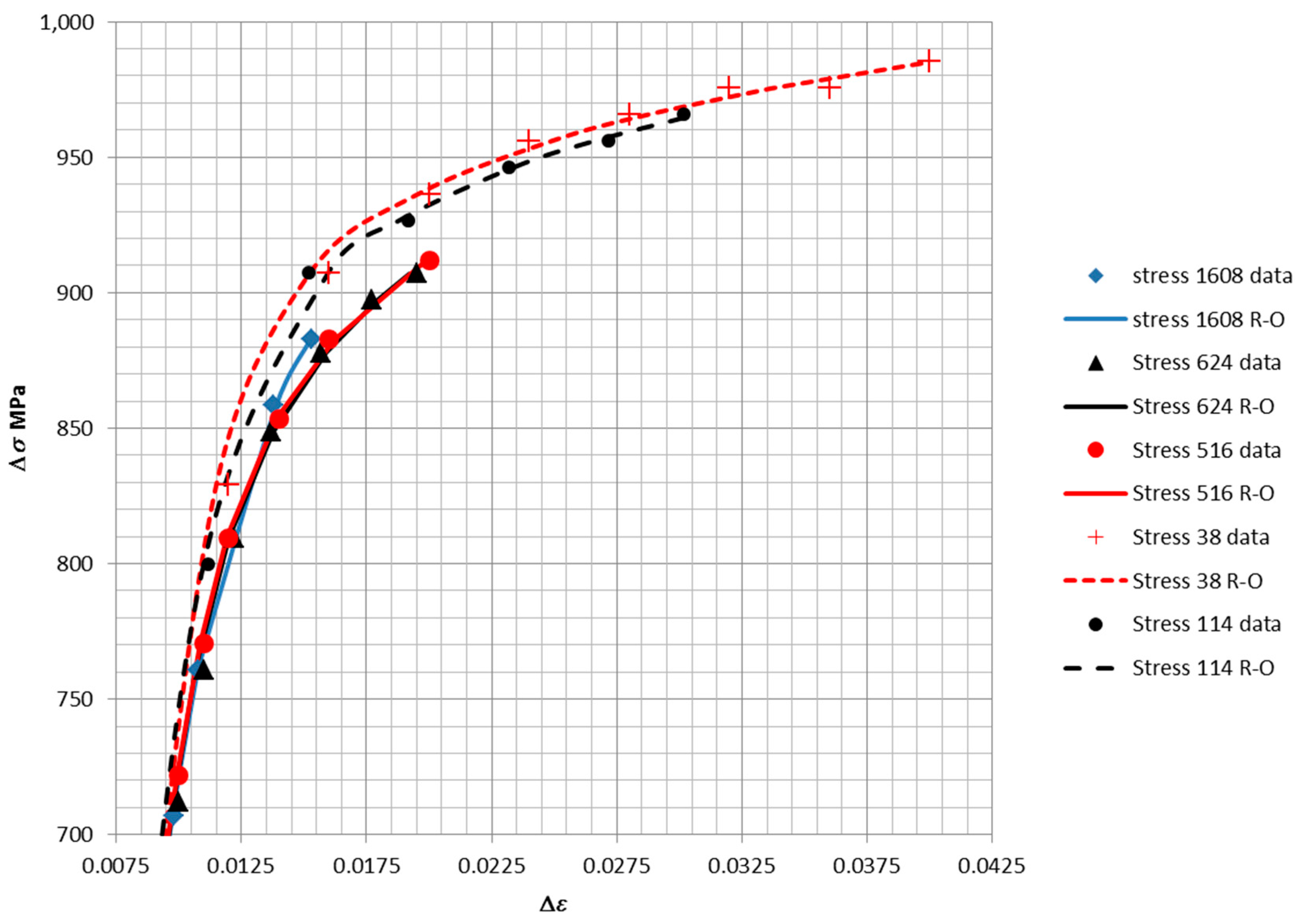
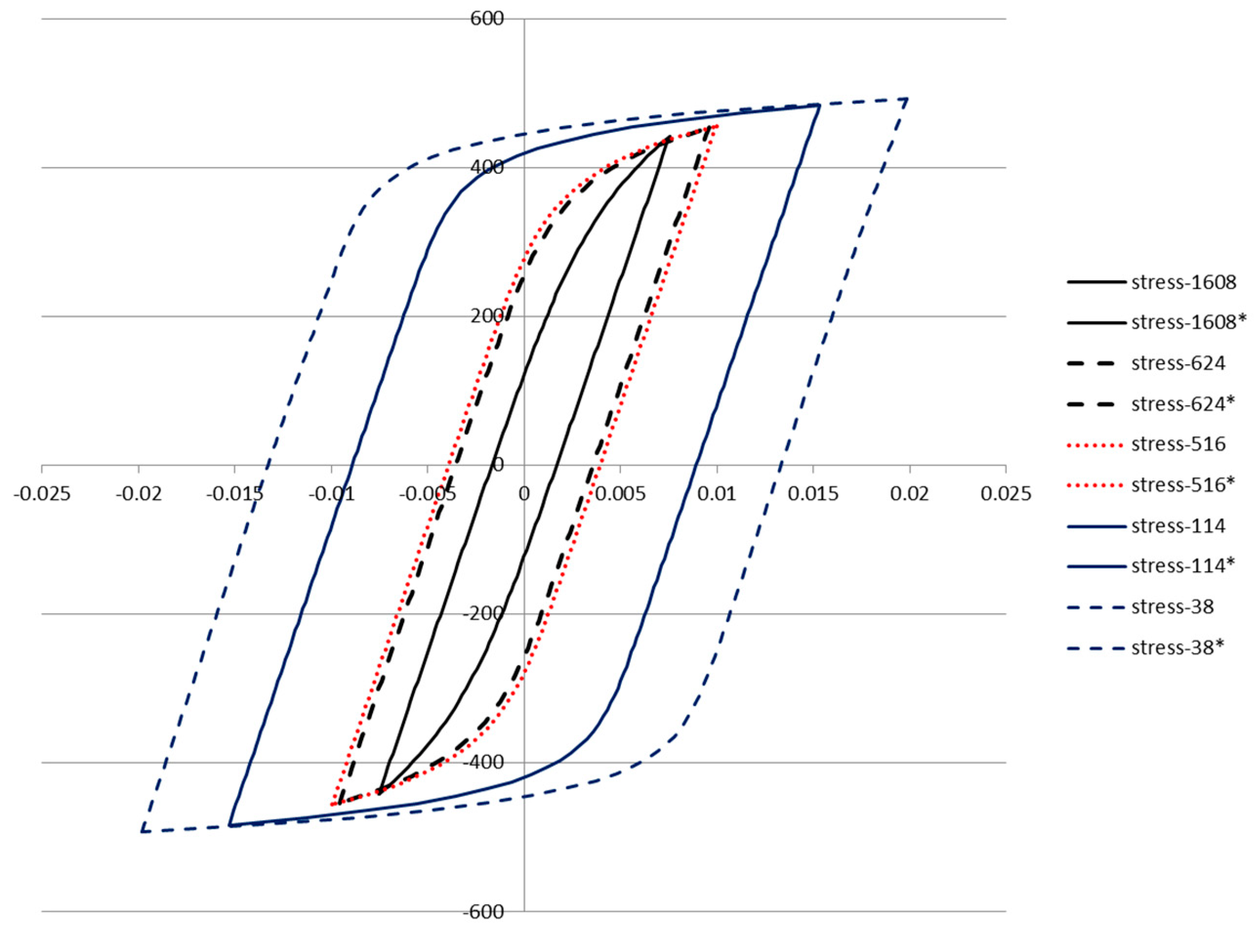
The fits of Equation (34) to loop data were performed using the least squares approach and is shown in
Figure 16. The fits to the data were of high accuracy, as demonstrated by the R
2 value of 0.997. This confirms that Equation (34) provides a reasonable model of the shape of the loops in
Figure 11,
Figure 12,
Figure 13,
Figure 14 and
Figure 15. The points are samples measured from the loops, while the line is the fit of Equation (34). A separate fit was performed for the parameters in Equation (34) for each of the five loops. A common value of Young’s modulus was fit simultaneously to the five sets of data. Specific values of
n and
K were obtained for each loop.
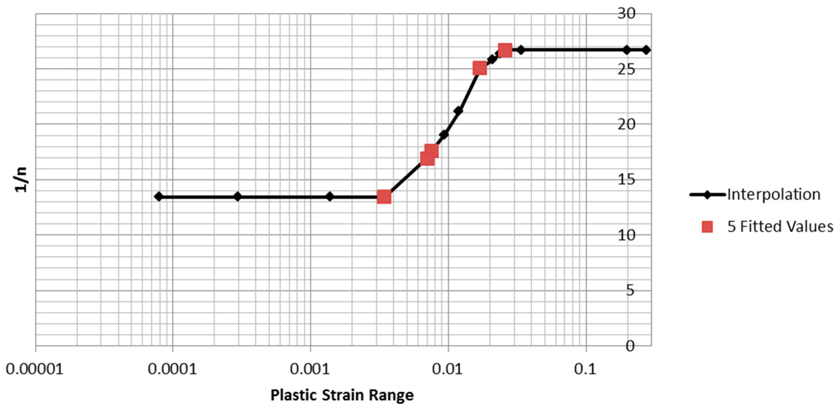
The five sets of parameters obtained from the fitted loops were used to estimate the parameter
1/n for the remaining 15 tests. The fitted
1/n value was found to be a strictly increasing function of plastic strain range, and is plotted in
Figure 17. The “interpolation” line markers show the values of
1/n used for the remaining 15 tests. The values were linearly interpolated between the maximum and minimum values. For plastic strain ranges outside the range of the measured data, the value of the nearest measured data value was used. As will be shown below, the predicted inelastic dissipation is mainly determined by the plastic strain range and the stress range, and is only weakly dependent on the value of
1/n used.
The five loops (represented by Equation (34)) are plotted in
Figure 18 below using the parameters fit to the corresponding loop data. The inelastic dissipation per cycle is the area enclosed by the loop.
The area of the loop in terms of the parameters in Equation (34) and the loading parameters are given in Equation (35). The form of this equation has the advantage that it is relatively robust to errors in fitting the parameter n, since both of the actual measured values of the stress range and strain range are used.
The loop area (dissipation per cycle) in terms of
n is [
23]:
In the present case, we wish to describe the evolution of damage in terms of reversals rather than cycles. It is apparent from Equation (36) that the inelastic dissipation per reversal is half the area of the loop given by Equation (35), and is given in Equation (37).
Total inelastic dissipation in terms of cycles and reversals:
Inelastic dissipation per reversal:
For specimens subjected to a monotonic test, the inelastic dissipation is the area under the plastic portion of the stress–strain curve. If the plastic portion of the curve is modeled by an equation of the form of Equation (34), the area under the plastic portion is given by Equation (38). A monotonic test to fracture can be interpreted as a fatigue test, with failure occurring after a single reversal. Thus, the inelastic dissipation per reversal is given by Equation (39):
The monotonic area (dissipation per reversal) in terms of
n:
The inelastic dissipation for a monotonic test:
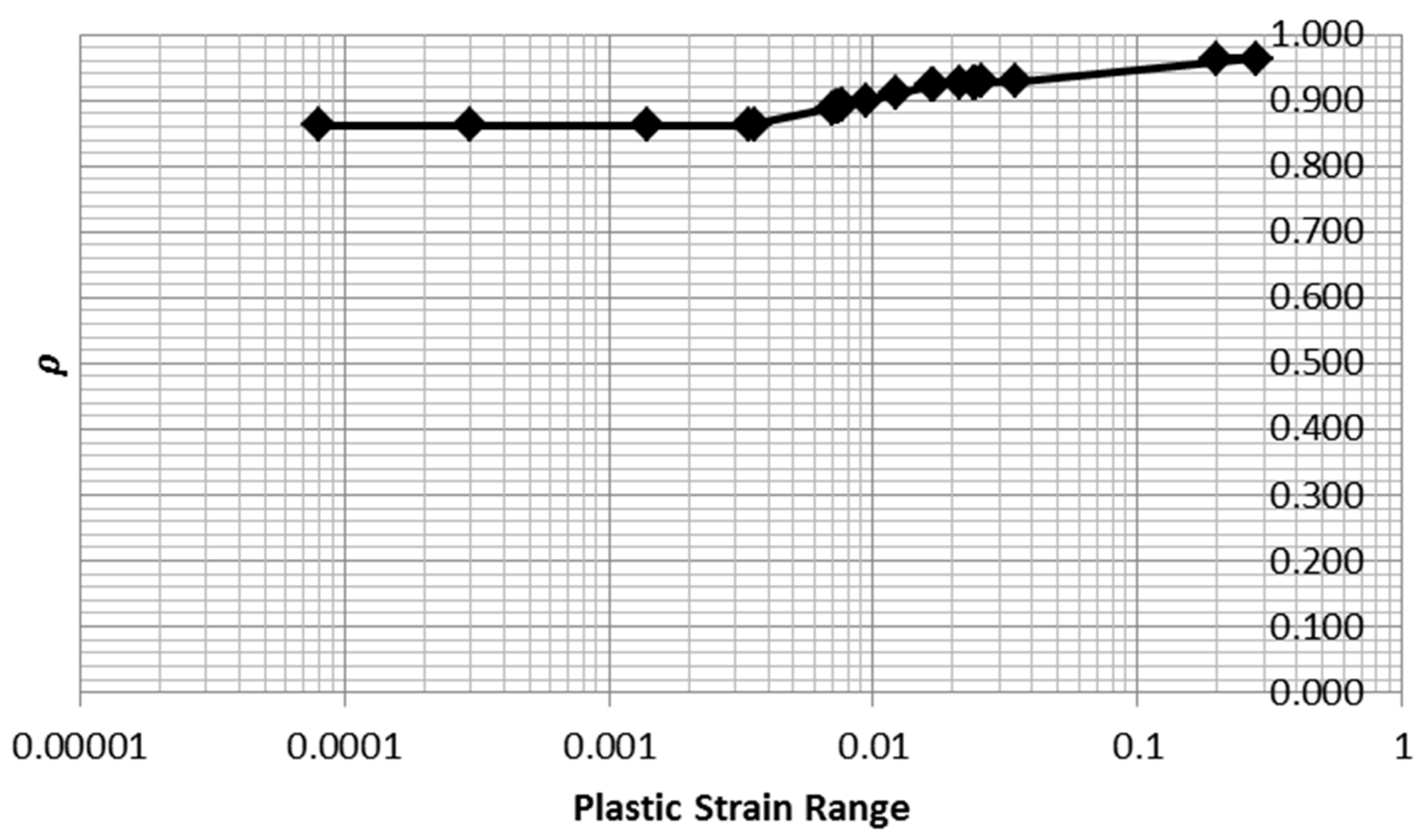
Note that in Equations (37) and (39), the area is computed from plastic strain range multiplied by stress range times a factor dependent on
n. The functions are given in Equation (40) and the values of
ρ are summarized in
Table 4 and plotted in
Figure 19.
Note that the value of ρ does not change greatly as n is varied. This observation indicates that the computation of areas for the monotonic and cyclic tests is robust to errors in fitting the Ramberg–Osgood parameter n. Thus, the inference of inelastic dissipation for the 15 tests for which loop data was not available is justified.
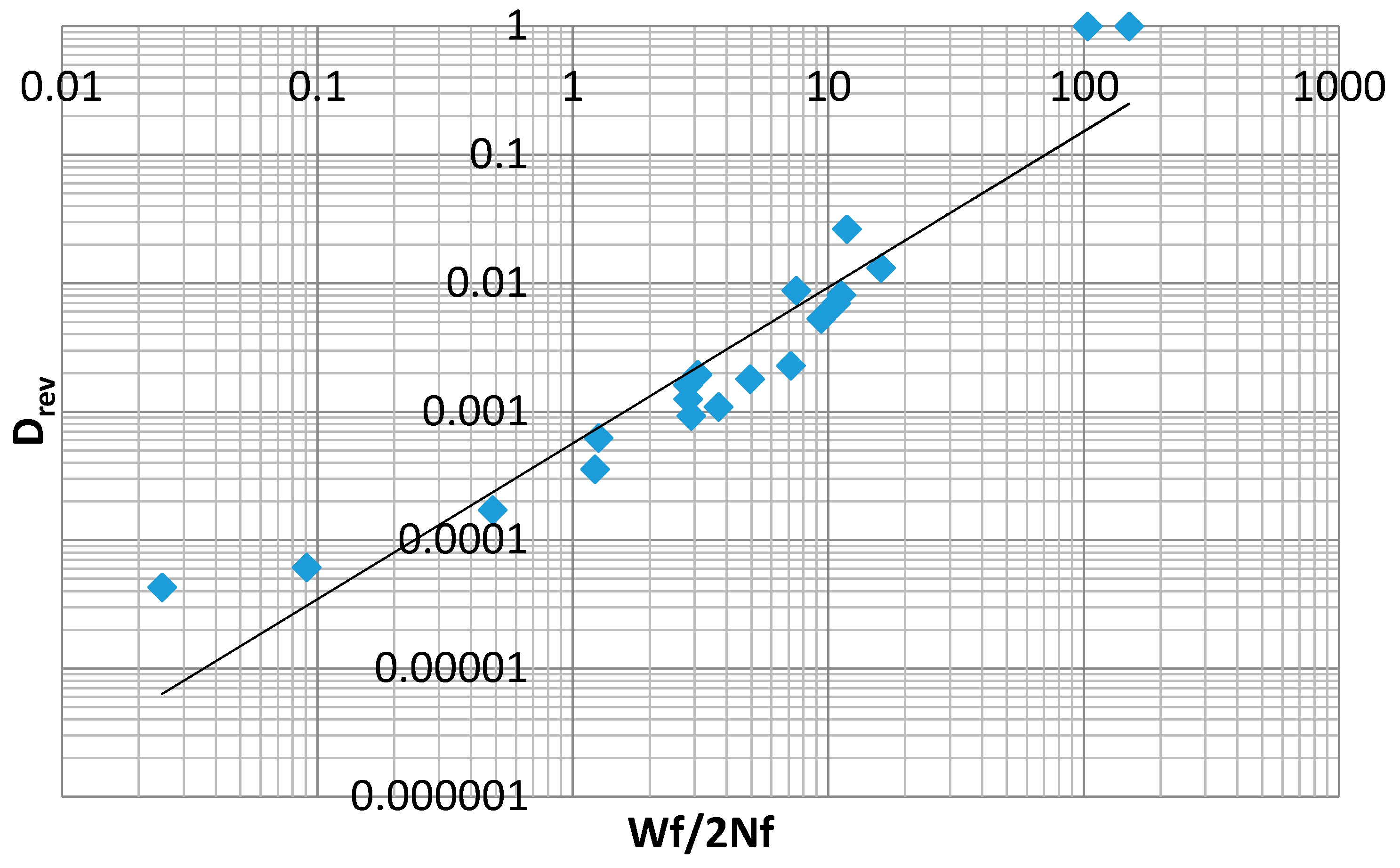
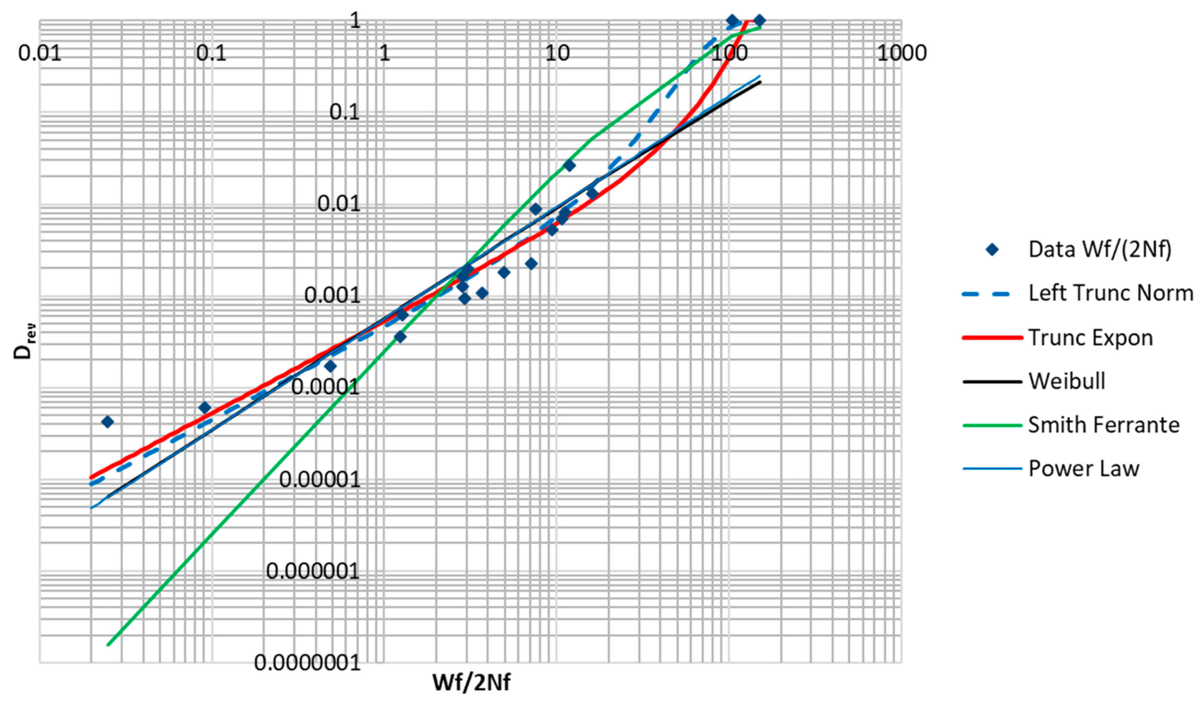
Table 3 below includes values computed from Equations (37) and (39) for inelastic dissipation per reversal, as well as damage per reversal, according to Equation (30). These data are plotted in
Figure 20. These points represent data corresponding to a relationship with the form of Equation (32). The lack of fit provided by the power law indicates that a different modeling equation is required for data of this type. In the development that follows, various expressions, including some based on MaxEnt principals, will be proposed to model the data plotted in
Figure 20.
Discussion of Candidate Distribution Functions
Inelastic dissipation is a non-negative-valued function, so only distribution functions equal to zero for
are admissible candidates.
Table 4 contains a summary of the fitted functions, as well as the sum of squares of error remaining after the fitting. The natural logs of the data were fitted to the natural logs of the predicted values. Plots of the fitted curves and the data are shown in
Figure 21. Only the truncated forms of the normal distribution are considered. Distributions that are truncated on the right, such as the truncated exponential distribution, have the additional advantage that they are strictly equal one for
.
The data set being fitted has some noteworthy features. Even though the data is of low-cycle fatigue, most of the samples still represent very small values of
. Additionally, the data points show a concave upwards trend that limits the quality of the fit achievable by a power law relationship. The fit was notably better for the right truncated exponential distribution with a negative
. The fitting procedure converged to a negative
, which corresponds to a rising exponential curve that becomes constant at
. The best fits were achieved by the truncated normal distribution and the truncated exponential distribution. The Smith–Ferrante function (popular in cohesive zone models of fracture) is typically used to represent the traction versus separation, and is founded on the relationship binding materials together at the microscopic scale [
24]. Its integral is used here, which has the qualitative features of a damage function. The Weibull distribution function was also tried. Additionally, a power law expression having the form of the Coffin–Manson relation was tried. This function would be truncated at
.
Note that the Coffin–Manson expression typically relates plastic strain range to cycles to failure. In
Table 4, it is shown in an inverted form and expressed in terms of
. It is clear from the sum of squared error column in
Table 4 and from
Figure 21 below that the truncated normal distribution provided the best fit to the data, followed by the truncated exponential distribution. The (inverted) Coffin–Manson expression and the Weibull distribution function provided the next best fits.
Parameters fit by numerical solver to the fatigue data for the truncated normal distribution (Equation (41)) and the truncated exponential distribution (Equation (42)) are given below:
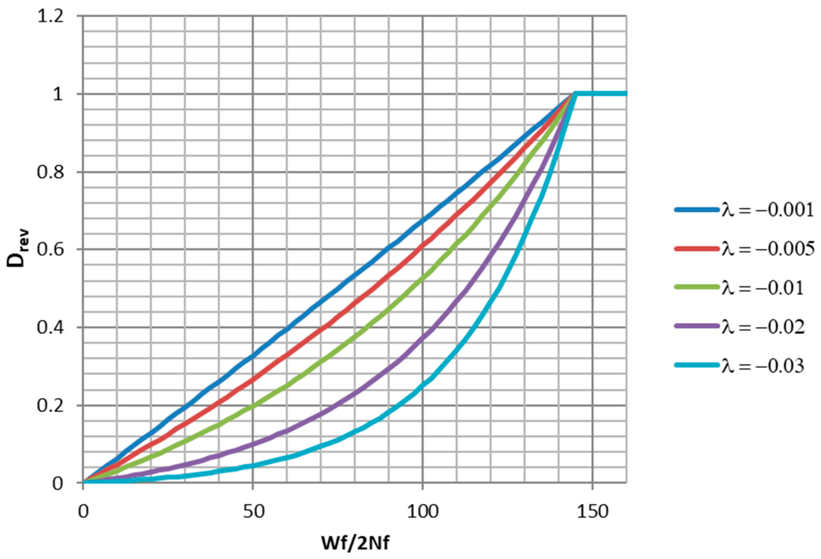
Although the trunated normal distribution has the best fit, the truncated exponential distribution has some desireable properties. If monotonic tension data points are available, they can be used to directly constrain the point where the curve is strictly equal to 1.0. The parameter
controls the shape of the curve between
and
. For
close to zero, the curve is nearly a ramp function. For negative
values, it has varying degrees of concave upwards curvature. Examples of a family of such curves are plotted in
Figure 22. In the present case,
, giving a strongly rising curve. A damage function of the mathematical form of Equation (42) exists in the literature [
2]. The authors of [
2] present Equation (43) as an improvement to the Coffin–Manson relationship (Equation (2)) for modeling LCF in the sub 100 cycle range (
is the plastic strain amplitude). The relationship is presented as an empirical improvement and is not derived from physical principles. The authors do not describe it as a truncated exponential distribution function. It is clear that Equation (43) can be rearranged to a form similar to Equation (42).


