Abstract
How to analytically deal with the entanglement and coherence dynamics of separated Jaynes–Cummings nodes with continuous-variable fields is still an open question. We here generalize this model to a more common situation including either a small or large qubit-field detuning, and obtain two new analytical formulas. The X-state simplification, Fock-state shortcut and detuning-limit approximation work together in an amazingly accurate way, which agrees with the numerical results. The new formulas almost perfectly predict the two-qubit entanglement dynamics both in sudden death and rebirth phenomenon for detuning interactions. We find that when both the qubit-field detuning and amplitude of coherent states are large enough, the maximal entanglement and coherence peaks can be fully and periodically retrieved, and their revival periods both increase linearly with the increasing detuning.
1. Introduction
Qubit entanglement and coherence preservation are core issues in the fundamental theory and experiment of quantum optics and quantum information [1,2,3,4,5,6,7,8,9,10,11,12,13,14,15,16,17,18,19,20,21,22,23,24]. Reliable operations in quantum information processing should rely on the coherent manipulation of which information is processed or transmitted [25,26]. However, due to decoherence, where the unavoidable coupling between the real quantum system and its surrounding environment chaotically changes the target quantum state and finally disappearances of entanglement and coherence occur, quantum entanglement and coherence become so fragile and consequently go through an asymptotic decay or a sudden death [27,28,29,30].
Previous studies [5,14,20,29] have shown that the entanglement sudden death and rebirth appear in two separate Jaynes–Cummings nodes where two initial fields are both in the vacuum states, which are tough to generate and preserve due to decoherence in real experiments. The node represents the quantum subsystem of interest, i.e., a qubit and a local quantum field. Furthermore, the so-called nodes should be initially entangled in order to observe death and rebirth (revivals) of entanglement. We focus on qubit entanglement in this paper. Therefore, it is significantly important to look for powerful field resources that can lead to the long-time generation and preservation of qubit entanglement and coherence.
One common continuous-variable resource is coherent state, which contains infinite eigenstate spectrums and can be easily controlled by a classical monochromatic current in real experiments [31,32]. However, although it can be solved directly through numerical diagonalization in a truncated Hilbert space, it is still difficult to obtain the analytical time-dependent dynamics when coupled to qubits due to the complexity of infinite-dimensional Hilbert space. As far as we know, how to analytically deal with the general entanglement and coherence dynamics of separated Jaynes–Cummings nodes with coherent-state fields is still an open question [33,34,35,36,37,38], and few analytical methods can be directly used to explain their entanglement and coherence dynamics.
It has been theoretically reported [35] that one-ebit entanglement reciprocation between qubits and coherent-state fields is workable by postselection, where this postselection needs an extra step to project a mixed state into a pure state. Recent works [37,38] use an analytically novel method to prove that, even when the amplitudes of coherent-state fields are both large enough, the qubit entanglement dynamics of two resonant Jaynes–Cummings nodes can be simply explained by an exponentially decaying formula. However, due to analytical diagonalization obstacle in the infinite-dimension Hilbert space, the above analytical formula fails completely when the qubit-field interaction is not resonant, and whether the coherence and one-ebit entanglement under the detuning interaction can be fully revived is unknown yet .
To answer the above question, we here focus on generalizing the saddle point method in [38] to a more common situation including either a small or large qubit-field detuning, and obtain two new formulas analytically describing the qubit entanglement dynamics. The new formulas well explain the two-qubit entanglement dynamics both in the sudden death and in the rebirth phenomenon when the qubit-field interaction is not resonant. Especially, we find that when both the detuning and amplitude of coherent states are large enough, the maximal entanglement and coherence peaks can be fully and periodically retrieved, and their revival periods both increase linearly with the increasing detuning. When qubit-field detuning is small enough, the two-qubit entanglement exhibits the sudden death and rebirth phenomenon, and its revival peaks increase quadratically with the increasing detuning, but the revival period is delayed with a quantity quadratically depending on the detuning, while its coherence quickly oscillates and exponentially decays without sudden death and rebirth. Finally, the effect of dissipation factors on the qubit entanglement is considered.
2. Hamiltonian System
As shown in Figure 1, the system is described by the double Jaynes–Cummings Hamiltonian ()
where is the transition frequency between the high level and low level of the qubit x (). and are Pauli matrices of the qubit x. (a) and (b) are the creation (annihilation) operators for two single-mode fields with angular frequency , respectively. G is the qubit-field coupling strength. Here the assumption , referred to as the system allowing nonzero qubit-field detuning, represents a clear distinction from the previous work with resonant coupling [38]. For simplicity, we define the detuning and transform the original Hamiltonian H into under the interaction picture as
where and (). We adopt Wootters concurrence C [39] as the two-qubit entanglement measure. In order to derive new approximate formulas for the detuning situatuion, we start to analyze two-qubit entanglement dynamics under a special situation, where the field modes are initially in their coherent states with zero amplitude, i.e., vacuum-state fields.
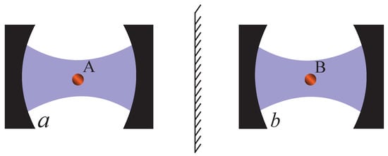
Figure 1.
(Color online) In the setup, qubits A and B couple to the fields a and b, respectively. There is not any interaction between A and B or between a and b.
2.1. Vacuum-State Fields
When the fields are initially in their vacuum states, the corresponding concurrence is
and its oscillation period is
Compared with Equation (27) of [38], the oscillation period of the expression C here has an approximately inverse relation with and becomes much smaller than that in Equation (27) of [38]. Figure 2a shows that the two-qubit entanglement keeps close to the maximum value for large detunings. Figure 2b shows that the period depends quadratically on the detuning, indicating that the entanglement oscillates more quickly when the detuning increases. These behaviors are very different from the system with resonant couplings [29] where the concurrence exhibits a standard Rabi oscillation with a fixed period. This is because detuning reduces the energy-exchange probability between the qubit and its local photon field, changing the period and amplitude of the Rabi oscillation. As the detuning increases, the energy coupling between entangled qubits and their respective vacuum states is very week, and the excitation energy mainly keeps in two qubits as the evolution time increases, ensuring two qubits are always in the originally entangled state.
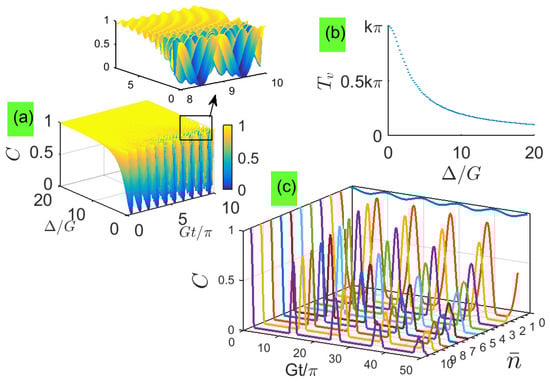
Figure 2.
(Color online) For different detunings: (a) Time dependence of concurrence. (b) Period of concurrence. (c) The dynamics of the concurrence for increasing the average photon number , where is starting from 0 (vacuum). To see periodic oscillations in Figure 2a clearly, a local-zoom subfigure is inserted in its top right-hand corner.
To provide examples in which the effect of the Stark shift can be clearly identified, the dynamics of the concurrence for increasing the average photon number is plotted in Figure 2c, where is starting from 0 (vacuum). When , the Stark shift can be clearly identified that the concurrence can not remain at 1 and becomes smaller as the evolution time is longer.
To explain the above results, it is necessary to make a further simplification for the analytical concurrence in the limit of small or large detuning. In the small-detuning limit, , leading to
and
which demonstrates that both the minimum value and period of concurrence are quadratically dependent on . In the large-detuning limit, , leading to and , which demonstrates that the concurrence keeps close to 1 and the period becomes reversely proportional to , explaining the fast-oscillation behavior in the concurrence. For the two-qubit coherence, its analytical result is the same to concurrence, and the effect of dissipation will exponentially reduce the two-qubit entanglement, i.e., when as proved in Equation (47) later.
In the followings, we focus on the system including two initial coherent-state fields with large amplitudes.
2.2. Coherent-State Fields
Assume the initial state of system to be
where the first qubit and the first field state are in order of listing, and the coherent state is expanded by the Fock states
Therefore, the evolution dynamics become
where
in which and . Since there is detuning in the infinite-dimension Hilbert space, the joint qubit-field dynamics in Equation (9) is extremely complicated and the generally analytical solution of concurrence is hard to obtain.
Our target here is to find new analytical formulas for determining the entanglement dynamics with highly excited (nearly classical) coherent-state fields. Under the limit of small or large detuning, the new formulas are intuitively drastic simplifications for infinite dimensions in the coherent-state fields and can explain new physics features which do not appear in the situation with resonant coupling.
Based on the idea of the Fock-state shortcut [38], when the average photon number of coherent-state fields satisfies , it is feasible to replace by , assuming that the photon number in each coherent state obeys the Poisson distribution and centers tightly around . Note that the qubit excitation (deexcitation) transition accompanies with the absorption (emission) of one photon, the initial field state can be equivalent to the single-product Fock state and the photon number in each field mode can be or during the resonant Jaynes–Cummings interaction. Consider the coherent oscillation between and , many other quantum states with different photon numbers are truncated in the following results. Actually, these results would only be correct when the energies of the two states are close to each other and those of others are not. If it is not the case, additional quantum states could be involved in the oscillation and the following simple results would break down. However, the detuning interaction causes a virtual energy exchange between the qubit and field mode, which enhances the validity of the above assumption, meaning that the photon number centers more tightly around in the detuning situation than that in the resonant situation.
By tracing out two field modes from Equation (9), we obtain the approximate X-form reduced density matrix of two qubits within as follows
where is the conjugate complex of and the other small-quantity elements denoted by are omitted through the equal- approximation. Thus, the concurrence has a simple form
Joint control of the coherent states and detuning will cause the time-dependent variation of matrix elements , and , leading to the growth or decline of two-qubit entanglement, which allows an extra freedom of detuning for controlling the entanglement than the resonant situation. Since the reduced density matrix in Equation (11) for two-qubit entanglement has been obtained by the method of Fock-state shortcut, we avoid using this method again and introduce another approximation method to obtain new analytic formulas for , and in the limit of small or large detuning.
It is workable to give out the fully analytical expressions of the elements in Equation (11) through the tracing operation . The result shows that the doubly infinite summations for , and are given as
and
respectively. These summations indicate that the qubits couple to an unclosed space of infinite states and the detuning mainly causes a nonlinear effect during the coupling process. It is not possible to complete these summations under general conditions, but their analytical solutions can be found when the coherent states are nearly classical under two limits, i.e., the limit of small or large detuning.
To approximate infinite summations into integrals, the Stirling equation is used to replace the term as follows
When , it is feasible to introduce an error-deviation order of centering near the Poisson peak and the terms . Thus we obtain the simplification form for infinite summations
and
Note that in Equation (18) is valid for any detuning. To further simplify the above summations, we rewrite as
and the approximation of large is used for expanding the term in Equation (19)
which transforms into
Similarly, the other useful approximations are
With these approximations and the identities
and
we can simplify the concurrence further as
Since the detuning appears in the square root of the Lambert W function [see Appendix (A1)–(A4)], it is impossible to fully calculate analytical results for the summations in Equation (27) under a general detuning by the saddle point method. However, we find that for the limit of small or large detuning, it is feasible to calculate analytically these summations through writing them as integrals, where the discrete integer n is treated as continuous when is large enough.
In the following section, we focus on exploring the concurrence in two limits of detuning that can be analytically treated by the saddle point method.
2.2.1. Small-Detuning Limit
The first extreme situation we focus on is the small-detuning limit, i.e., . Under this limit, the summations in Equation (27) can be simplified further as
where is used and high-order terms than have been omitted. Therefore, it needs to calculate four integrals
and
These integrals can be combined as and for dealing with the exponentials and , respectively. Based on the Stirling equation and Euler formula, the integrals can be approximated as
and
It is workable to use the saddle point method [38] to analytically calculate the integrals and , and details for dealing with small-detuning terms of the exponentials are contained in the Appendix (A5)–(A34). Thus, analytical expressions for and are found to be
and
where . By putting these approximation results into Equation (28), a new formula for two-qubit entanglement determiner with small detunings is obtained
For this formula we have used the fact that only the term with the corresponding k around or gives a main contribution to the sums. Compared with Equation (60) of [38], this formula here in Equation (37) contains new contributions of in the index of exponential function and the period of cosine function. The contribution to or from any other decays exponentially with the distance from k, i.e., proportional to
which decays with the square of increasing detuning. This leads to the unique revival period and the relative revival envelope height
Compared with Equation (61) of [38], this formula here in Equation (39) contains a new contribution in the index of exponential function, and the relative revival envelope height grows with the increasing . Thus the formula in Equation (37) is the main analytical result for each step index k with small detuning and reduces to that with resonant coupling [38] at both the decay exponent and revival period, where resonance can be viewed as a special limit of small detuning.
To perform the numerical simulations, we use the Hamiltonian given in Equation (2) by truncating the Fock basis and calculating the reduced density matrix in each excitation subspace, then summing over all the subspaces to get the total reduced density matrix. This Fock-basis truncation is based on the precision accuracy of numerical concurrence, and the total excitation number is cut off at . For example, when coherent states contain bosons in each of the cavity modes, the total excitation number is cut off at 200. This is because when , the width of the photon number distribution obeys . Therefore, it is safe to make this Fock-basis truncation.
In Figure 3a,b, we plot the long-time entanglement dynamics with small detunings for analytical and numerical calculations when two qubits are exposed to two coherent fields each with a large average photon number , respectively. In Figure 3c, value is the first concurrence revival peak. We find that the entanglement exhibits sudden death and rebirth phenomenon, and its revival peaks are not fully complete but increase quadratically with the increasing detuning, as shown in Figure 3c. The revival period is delayed with a quantity quadratically depending on the detuning, as shown in Figure 3d. The numerical results in Figure 3b are not perfectly predicted by the corresponding analytical results in Figure 3a, and their main difference is the absence of Rabi-type oscillations during the revivals, i.e., the disappearance of tiny revivals in numerical results, which are not contained in the new formula of Equation (37). This is because the entanglement between the two subsystems is conserved due to no interaction between them. The small detuning in each subsystem makes each photon field deviate from the coherent state so that an ebit for the qubits cannot be completely transferred to the fields, i.e., two qubits become a mixed state and their entanglement quickly vanishes by tracing out two fields as the evolution time increases, so that the two qubits can not be fully recovered.
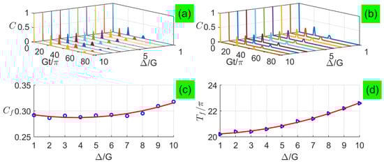
Figure 3.
(Color online) Concurrence as a function of the evolution time under small detunings with : (a) analytical results and (b) numerical results, where analytical results are plotted based on Equation (37). Characteristics of the first revival envelope versus small detunings: (c) peaks and (d) periods .
2.2.2. Large-Detuning Limit
The second extreme situation we focus on is the large-detuning limit, i.e., . Under this limit, the summations in Equation (27) can be simplified further as
where is used and higher-order terms than have been omitted. We need to recalculate the integrals in Equations (33) and (34), where large-detuning terms can be directly removed from the square root of the Lambert W function, and these derivation details are contained in the Appendix (A35)–(A48). We obtain the analytical expressions of and as follows
and
With these results in Equation (40), a new formula for two-qubit entanglement determiner with large detunings is obtained
Here, different from the cases of resonance and small detuning, the principal exponential exhibits a periodical oscillation between the minimum and the maximum values, and does not decay monotonously with the increasing time, giving a main contribution to the sums around , where does not depend on the average photon number. It is interesting to see that around , the relative revival envelope height is the maximum concurrence , meaning that the entanglement recovery can be fully complete without any postselection operation. This result is surprisingly different from the result with resonance or small detuning where the maximal entanglement is never fully complete.
In Figure 4a,b, we plot the long-time entanglement dynamics with large detunings for analytical and numerical calculations when two qubits are exposed to two coherent fields with a large average photon number , respectively. We find that the two-qubit entanglement also exhibits sudden death and rebirth phenomenon, and its revival peaks are fully complete without depending on the detuning, but the revival period increases linearly with the increasing detuning, as shown in Figure 4c,d. Although the new formula here is very different from that in the small-detuning limit, only the absence of Rabi-type oscillations during the revivals of numerical results in Figure 4b are not perfectly predicted by the corresponding analytical results in Figure 4a, which is generically similar to the revivals presented for one qubit inversion of quantum revivals with detunings [40].
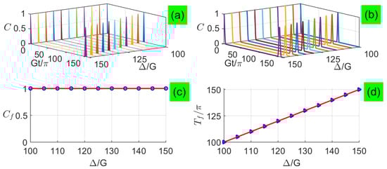
Figure 4.
(Color online) Concurrence as a function of the evolution time under large detunings with : (a) analytical results and (b) numerical results, where analytical results are plotted based on Equation (43). Characteristics of the first revival envelope versus large detunings: (c) peaks and (d) periods .
The physics explanation is that under the large-detuning limit, the dispersive interaction between the qubit and field causes a Stark movement in the field frequency, which depends on the qubit state. This Stark movement leads to the opposite phase shifts between two field components, which generates entanglement between the qubit and field. When this phase difference accumulates to a certain extent, the qubit and field approximately becomes the maximally entangled state, but two qubits become a mixed state and their entanglement vanishes by tracing out two fields. However, when this phase difference is , the qubit and field are not entangled and the two-qubit entanglement can be fully recovered. While in the small-detuning limit, this phase difference is impossible to achieve and the two qubits can not be fully recovered. This physical process has an essential difference with that of virtual energy exchanging realized for two qubits and one vacuum field in cavity-quantum-electrodynamics system [41,42].
2.2.3. Further Discussion
To see the transition from small to large detunings, we numerically simulate the concurrence dynamics for general detunings in Figure 5. From Figure 5a, it is obviously to see that each concurrence curve has a similar revival pattern and changes regularly from small to large detunings. Although the above method cannot analytically predict the concurrence dynamics for moderate detunings, it is still possible to mathematically fit the characteristics of the first revival envelope when it transits from small to large detunings. By mathematically fitting the first revival envelope in Figure 5b,c, it is interesting to find that the revival peak quadratically depends on the detuning, but the revival period linearly relates with the detuning. This result exhibits a detuning-dependence discrepancy with that under the small or large detuning.
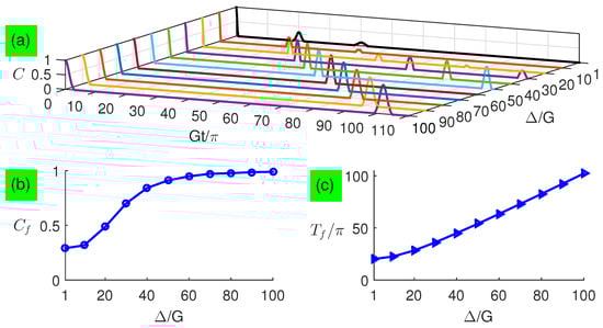
Figure 5.
(Color online) (a) Concurrence as a function of the evolution time for general detunings with . Characteristics of the first revival envelope versus moderate detunings: (b) peaks and (c) periods .
To quantitatively show the quasiperiodic modulations by other amplitudes of the coherent state, we plot the concurrence dynamics with other average photon numbers in Figure 6. In Figure 6a,b, detuning modulation exhibits with different revival periods. For small detunings in Figure 6c, the revival period increases linearly with the increasing , i.e., . For large detunings in Figure 6d, the revival period has a fixed value without depending on and the increasing narrows the revival envelope in the time domain. Even when decreases to 25, the analytical results well predict the numerical results. This result demonstrates that two new formulas in Equations (37) and (43) are workable for a wide range of the average photon number.
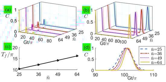
Figure 6.
(Color online) Concurrence as a function of the evolution time for average photon number with: (a) and (b) . In each pair of curves with the same , the numerical result is plotted in front and the analytical result is plotted behind, where the analytical results in subfigures (a) and (b) are based on Equations (37) and (43) respectively. (c) Period of the first revival envelope versus average photon number for . (d) Concurrence dynamics of the first revival envelope versus average photon number for .
2.3. Quantum Coherence
Another important issue is to answer the question of whether it is possible to fully recover the coherence of two qubits from the infinite-dimension fields, i.e., coherent-state fields. To answer this question, we examine the two-qubit coherence mainly caused by detuning modulations in this section.
We first assess the quantum coherence dynamics of two qubits by computing the norm of coherence [43], where is off-diagonal elements of density matrix in the basis . In general, , where d is the dimension of . According to Equation (11), we obtain the analytical expression of , which takes a simple form , and . The analytical formula of coherence for the small-detuning limit is ()
while for the large-detuning limit is ()
In Figure 7, we numerically simulate the long-time dynamics of two-qubit coherence with small and large detunings. For the small-detuning limit, we find that the coherence increases from to its maximum around the time , i.e., two qubits evolve from their maximally entangled state to maximally coherent state , then decay exponentially to zero with the increasing time. In contrast, for the large-detuning limit, we find that the coherence has an initially high value and exponentially decays to a relatively low non-zero value at the beginning. After a time period , the coherence is fully recovered to the initial high value, i.e., two qubits evolve to a state between the maximally entangled and maximally coherent states. This result is qualitatively different from the concurrence result. When the detuning is large, the coherence remains nonzero during the vanishing of entanglement, which does not exhibit the sudden death phenomenon. But, when the detuning is small, the coherence may inversely increase during the vanishing of entanglement.
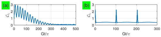
Figure 7.
(Color online) as a function of the evolution time with for: (a) and (b) .
It is of interest to see what the photon states are when the qubit states evolve to a maximal coherence and minimal coherence. In Figure 8, we plot the evolution dynamics of the average photon number and width in distribution. We find that the average photon number for each subsystem becomes maximum when the qubit states evolve to a maximal coherence, but becomes minimum when the qubit states evolve to a minimal coherence, and width in distribution has the similar evolution with that in the qubit coherence.
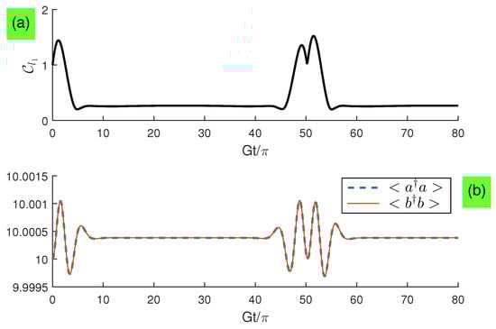
Figure 8.
(Color online) Evolution dynamics with and for: (a) ; (b) and .
3. Effect of Dissipation
To see the effect of dissipation factors on the two-qubit entanglement, we numerically simulate the system’s master equation by the approach of quantum trajectory [44]. This approach assumes that when the system contains the rates of photon decay and qubit spontaneous emission , the system evolves approximately under a non-Hermitian Hamiltonian
where , , , and are the collapse operators causing instantaneous quantum jumps. Equation (46) is a Hamiltonian interaction in the Schrödinger picture, where the operator is time-independent but the state vector is time-dependent.
In Figure 9, we numerically simulate the effect of dissipation factor or on the two-qubit entanglement both for small and large detunings. The result shows that the entanglement decreases exponentially as or increases, and is more robust against the qubit spontaneous emission than photon decay. To explain this exponential decay behavior of entanglement, it is necessary to make an assumption for obtaining the analytical solution
where a new factor appears compared with the original concurrence . This factor has a decreasing exponential parameter linear with dissipation rates and square with the amplitude of coherent states, which causes exponential decays in the original concurrence.
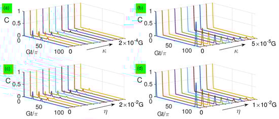
Figure 9.
(Color online) Numerical simulation of entanglement dynamics based on Equation (46) when : (a) and ; (b) and ; (c) and ; (d) and . Black arrows point to the direction of increasing dissipation.
4. Conclusion
This paper generalizes the method reported in [38], which was restricted to the resonant situation, to a more general situation including qubit-field detunings. Based on numerical simulations and analytically new formulas, we demonstrate that the X-state simplification, Fock-state shortcut and detuning-limit approximation work together in an amazingly accurate way, which agrees with the numerical results. Although the numerical to analytic agreements are not perfect, it is safe to say that the new formulas can predict the numerical results under a wide range of average photon numbers in the coherent state. Especially, we find that when both the detuning and amplitude of coherent states are large enough, the maximal entanglement and coherence peaks can be fully and periodically retrieved and their revival periods both increase linearly with the increasing detuning. Finally, the effect of dissipation factors on the qubit entanglement is analyzed.
The work is important because the new formulas reveal the analytical relation between the entanglement evolution dynamics and detunings, which further clarifies the physics mechanism of entanglement sudden death and rebirth and provides a basic solution for direct use in any real systems. In the future, we want to further study the situation with more qubits and try to seek a general detuning solution under special continuous variables.
Author Contributions
All authors contributed equally to this article. The theoretical aspect of this work does not allow to point any substantial authorship. All authors have read and approved the final manuscript.
Funding
This work is supported by the National Natural Science Foundation of China under Grant (Grant Nos. 11674060, 11705030, and 11875108), the Natural Science Foundation of Fujian Province (Grant Nos. 2017J05005 and 2018J01412), and the fund from Fuzhou University (Grant No. XRC-1566).
Conflicts of Interest
The authors declare no conflict of interest.
Appendix A
Based on the saddle point method [38], if M is a large number and is a twice-differentiable function, an integral can be approximated as
where corresponds to the global maximum of .
When , we analyze the saddle point method used in calculating the integrals of and as follows. For the integral
where
We choose to find the maximum value . For this, we need to find the point to satisfy
Different from the resonant situation, since the detuning appears in the square root of the Lambert W function, it is impossible to completely calculate analytical results for Equation (A4) under general detunings. However, when and , Equation (A4) can be simplified as
To solve Equation (A5), it is helpful to separate the modulus and phase
then Equation (A5) becomes
By equalling the real and imaginary parts of two sides in Equation (A7), we obtain a set of solutions by omitting higher-order terms than as
With this solution, Equation (A3) becomes
By inserting for , we obtain
The final term to calculate is
where higher-order terms than have been omitted. Therefore, the analytical solution of approximates
leading to the summations
and
where .
Now, we turn to the integral
We will again use the saddle point method to find the maximum of the function
and should find the point to satisfy
Similarly, when is small enough, Equation (A17) is simplified as
Letting , then
where the real and imaginary equations become
For , where k is a positive integer, the above equations become
Let and , where and . When and are small, the equations in Equation (A20) turn into
By inserting into Equation (A16), we get
The real part of Equation (A23) is
By inserting and omitting higher-order terms than in Equation (A24),
By substituting with and retaining only the terms up the second order in for Equation (A25),
Similarly, the imaginary part of is
Again, by inserting and , substituting with , and retaining the terms up the second order in for Equation (A27),
The final term to calculate is
which has two forms: one for ,
and the other for
For , we make another approximation , leading to
Different from the small-detuning limit, this equation is analytically solvable for , leading to
where the terms higher-order than have been omitted through the Taylor expansion. With this solution, Equation (A3) becomes
and becomes
This equation is directly solvable for and we find
Since the exponential becomes larger as the evolution time increases, this can not be expanded further and should be substituted fully into Equation (A3) as
and becomes
Note that the case of distinct coupling constants for different cavities has been done in [45], but the case of distinct detunings for different cavities is still an open question.
References
- Streltsov, A.; Rana, S.; Bera, M.N.; Lewenstein, M. Towards resource theory of coherence in distributed scenarios. Phys. Rev. X 2017, 7, 011024. [Google Scholar] [CrossRef]
- Černoch, A.; Bartkiewicz, K.; Lemr, K.; Soubusta, J. Experimental tests of coherence and entanglement conservation under unitary evolutions. Phys. Rev. A 2018, 97, 042305. [Google Scholar] [CrossRef]
- Humphreys, P.C.; Kalb, N.; Morits, J.P.J.; Schouten, R.N.; Vermeulen, R.F.L.; Twitchen, D.J.; Markham, M.; Hanson, R. Deterministic delivery of remote entanglement on a quantum network. Nature 2018, 558, 268. [Google Scholar] [CrossRef] [PubMed]
- Song, C.; Zheng, S.B.; Zhang, P.F.; Xu, K.; Zhang, L.; Guo, Q.J.; Liu, W.X.; Xu, D.; Deng, H.; Huang, K.Q.; et al. Continuous-variable geometric phase and its manipulation for quantum computation in a superconducting circuit. Nat. Commun. 2017, 8, 1061. [Google Scholar] [CrossRef] [PubMed]
- Brunner, N.; Cavalcanti, D.; Pironio, S.; Scarani, V.; Wehner, S. Bell nonlocality. Rev. Mod. Phys. 2014, 86, 419. [Google Scholar] [CrossRef]
- Franco, R.L.; Compagno, G. Indistinguishability of elementary systems as a resource for quantum information processing. Phys. Rev. Lett. 2018, 120, 240403. [Google Scholar] [CrossRef] [PubMed]
- Rab, A.S.; Polino, E.; Man, Z.X.; An, B.N.; Xia, Y.J.; Spagnolo, N.; Franco, R.L.; Sciarrino, F. Entanglement of photons in their dual wave-particle nature. Nat. Commun. 2017, 8, 915. [Google Scholar] [CrossRef]
- Xu, J.S.; Sun, K.; Li, C.F.; Xu, X.Y.; Guo, G.G.; Andersson, E.; Franco, R.L.; Compagno, G. Experimental recovery of quantum correlations in absence of system-environment back-action. Nat. Commun. 2013, 4, 2815. [Google Scholar] [CrossRef]
- Nosrati, F.; Castellini, A.; Compagno, G.; Franco, R.L. Control of noisy entanglement preparation through spatial indistinguishability. arXiv, 2019; arXiv:1907.00136. [Google Scholar]
- Eberly, J.H.; Yu, T. The end of an entanglement. Science 2007, 316, 555. [Google Scholar] [CrossRef]
- Mortezapour, A.; Naeimi, G.; Franco, R.L. Coherence and entanglement dynamics of vibrating qubits. Opt. Commun. 2018, 424, 26. [Google Scholar] [CrossRef]
- Mortezapour, A.; Borji, M.A.; Franco, R.L. Protecting entanglement by adjusting the velocities of moving qubits inside non-Markovian environments. Laser Phys. Lett. 2017, 14, 055201. [Google Scholar] [CrossRef]
- Plenio, M.B.; Virmani, S. An introduction to entanglement measures. Quantum Inf. Comput. 2007, 7, 1. [Google Scholar]
- Aolita, L.; de Melo, F.; Davidovich, L. Open-system dynamics of entanglement:a key issues review. Rep. Prog. Phys. 2015, 78, 042001. [Google Scholar] [CrossRef] [PubMed]
- Tsokeng, A.T.; Tchoffo, M.; Fai, L.C. Quantum correlations and decoherence dynamics for a qutrit-qutrit system under random telegraph noise. Quantum Inf. Comput. 2017, 16, 191. [Google Scholar] [CrossRef]
- González-Gutiérrez, C.A.; Román-Ancheyta, R.; Espitia, D.; Franco, L.R. Relations between entanglement and purity in non-Markovian dynamics. Int. J. Quantum Inform. 2016, 14, 1650031. [Google Scholar] [CrossRef]
- Dehghani, A.; Mojaveri, B.; Bahrbeig, R.J.; Nosrati, F.; Franco, L.R. Entanglement transfer in a noisy cavity network with parity-deformed fields. J. Opt. Soc. Am. B 2019, 36, 1858. [Google Scholar] [CrossRef]
- Dijkstra, A.G.; Tanimura, Y. Non-markovian entanglement dynamics in the presence of system-bath coherence. Phys. Rev. Lett. 2010, 104, 250401. [Google Scholar] [CrossRef]
- Mortezapour, A.; Franco, L.R. Protecting quantum resources via frequency modulation of qubits in leaky cavities. Sci. Rep. 2018, 8, 14304. [Google Scholar] [CrossRef] [PubMed]
- Lo Franco, R.; Compagno, G. Overview on the phenomenon of two-qubit entanglement revivals in classical environments. In Lectures on General Quantum Correlations and Their Applications; Fanchini, F., Adesso, G., Eds.; Quantum Science and Technology; Springer: Cham, Switzerland, 2017; pp. 367–391. [Google Scholar]
- Silva, I.A.; Souza, A.M.; Bromley, T.R.; Cianciaruso, M.; Marx, R.; Sarthour, R.S.; Oliveira, I.S.; Franco, R.L.; Glaser, S.J.; deAzevedo, E.R.; et al. Observation of time-invariant coherence in a nuclear magnetic resonance quantum simulator. Phys. Rev. Lett. 2016, 117, 160402. [Google Scholar] [CrossRef]
- Bromley, T.R.; Cianciaruso, M.; Adesso, G. Frozen quantum coherence. Phys. Rev. Lett. 2015, 114, 210401. [Google Scholar] [CrossRef] [PubMed]
- Chiuri, A.; Vallone, G.; Paternostro, M.; Mataloni, P. Extremal quantum correlations: Experimental study with two-qubit states. Phys. Rev. A 2011, 84, 020304(R). [Google Scholar] [CrossRef]
- Cornelio, M.F.; de Oliveira, M.C.; Fanchini, F.F. Entanglement irreversibility from quantum discord and quantum deficit. Phys. Rev. Lett. 2011, 107, 020502. [Google Scholar] [CrossRef] [PubMed]
- Körber, M.; Morin, O.; Langenfeld, S.; Neuzner, A.; Ritter, S.; Rempe, G. Decoherence-protected memory for a single-photon qubit. Nat. Photon. 2018, 12, 18. [Google Scholar] [CrossRef]
- Wang, Z.Y.; Casanova, J.; Plenio, M.B. Delayed entanglement echo for individual control of a large number of nuclear spins. Nat. Commun. 2017, 8, 14660. [Google Scholar] [CrossRef] [PubMed]
- Throckmorton, R.E.; Barnes, E.; Sarma, S.D. Environmental noise effects on entanglement fidelity of exchange-coupled semiconductor spin qubits. Phys. Rev. B 2017, 95, 085405. [Google Scholar] [CrossRef]
- Kaufmann, H.; Ruster, T.; Schmiegelow, C.T.; Luda, M.A.; Kaushal, V.; Schulz, J.; von Lindenfels, D.; Schmidt-Kaler, F.; Poschinger, U.G. Scalable creation of long-lived multipartite entanglement. Phys. Rev. Lett. 2017, 119, 150503. [Google Scholar] [CrossRef]
- Yu, T.; Eberly, J.H. Sudden death of entanglement. Science 2009, 323, 598. [Google Scholar] [CrossRef]
- Yu, T.; Eberly, J.H. Finite-time disentanglement via spontaneous emission. Phys. Rev. Lett. 2004, 93, 140404. [Google Scholar] [CrossRef]
- Braunstein, S.L.; van Loock, P. Quantum information with continuous variables. Rev. Mod. Phys. 2005, 77, 513. [Google Scholar] [CrossRef]
- Adesso, G.; Illuminati, F. Entanglement in continuous-variable systems: Recent advances and current perspectives. J. Phys. A 2007, 40, 7821. [Google Scholar] [CrossRef]
- Rafsanjani, S.M.H.; Eberly, J.H. Coherent control of multipartite entanglement. Phys. Rev. A 2015, 91, 012313. [Google Scholar] [CrossRef]
- Casagrande, F.; Lulli, A.; Paris, M.G. Improving the entanglement transfer from continuous-variable systems to localized qubits using non-Gaussian states. Phys. Rev. A 2007, 75, 032336. [Google Scholar] [CrossRef]
- Lee, J.; Paternostro, M.; Kim, M.S.; Bose, S. Entanglement reciprocation between qubits and continuous variables. Phys. Rev. Lett. 2006, 96, 080501. [Google Scholar] [CrossRef] [PubMed]
- Paternostro, M.; Kim, M.S.; Palma, G.M. Accumulation of entanglement in a continuous variable memory. Phys. Rev. Lett. 2007, 98, 140504. [Google Scholar] [CrossRef] [PubMed]
- Yönaç, M.; Eberly, J.H. Qubit entanglement driven by remote optical fields. Opt. Lett. 2008, 33, 270. [Google Scholar] [CrossRef]
- Yönaç, M.; Eberly, J.H. Coherent-state control of noninteracting quantum entanglement. Phys. Rev. A 2010, 82, 022321. [Google Scholar] [CrossRef]
- Wootters, W.K. Entanglement of formation of an arbitrary state of two qubits. Phys. Rev. Lett. 1998, 80, 2245. [Google Scholar] [CrossRef]
- Eberly, J.H.; Narozhny, N.B.; Sanchez-Mondragon, J.J. Periodic spontaneous collapse and revival in a simple quantum model. Phys. Rev. Lett. 1980, 44, 1323. [Google Scholar] [CrossRef]
- Zheng, S.B.; Guo, G.C. Efficient scheme for two-atom entanglement and quantum information processing in cavity QED. Phys. Rev. Lett. 2000, 85, 2392. [Google Scholar] [CrossRef]
- Osnaghi, S.; Bertet, P.; Auffeves, A.; Maioli, P.; Brune, M.; Raimond, J.M.; Haroche, S. Coherent control of an atomic collision in a cavity. Phys. Rev. Lett. 2001, 87, 037902. [Google Scholar] [CrossRef] [PubMed]
- Baumgratz, T.; Cramer, M.; Plenio, M.B. Quantifying coherence. Phys. Rev. Lett. 2014, 113, 140401. [Google Scholar] [CrossRef] [PubMed]
- Dalibard, J.; Castin, Y.; Mølmer, K. Wave-function approach to dissipative processes in quantum optics. Phys. Rev. Lett. 1992, 68, 580. [Google Scholar] [CrossRef] [PubMed]
- Shen, L.T.; Shi, Z.C.; Wu, H.Z.; Yang, Z.B. Dynamics of entanglement in Jaynes–Cummings nodes with nonidentical qubit-field coupling strengths. Entropy 2017, 19, 331. [Google Scholar] [CrossRef]
© 2019 by the authors. Licensee MDPI, Basel, Switzerland. This article is an open access article distributed under the terms and conditions of the Creative Commons Attribution (CC BY) license (http://creativecommons.org/licenses/by/4.0/).