Article

A New Chaotic System with Stable Equilibrium: Entropy Analysis, Parameter Estimation, and Circuit Design

1
Division of Dynamics, Lodz University of Technology, Stefanowskiego 1/15, 90-924 Lodz, Poland
2
Power Electronics and Renewable Energy Research Laboratory (PEARL), Department of Electrical Engineering, Faculty of Engineering, University of Malaya, Kuala Lumpur 50603, Malaysia
3
Department of Information Technology, Faculty of Computing and IT, King Abdulaziz University, Jeddah 21589, Saudi Arabia
4
Department of Mathematics, Quaid-I-Azam University 45320, Islamabad 44000, Pakistan
5
NAAM Research Group, King Abdulaziz University, Jeddah 21589, Saudi Arabia
6
Modeling Evolutionary Algorithms Simulation and Artificial Intelligence, Faculty of Electrical & Electronics Engineering, Ton Duc Thang University, Ho Chi Minh City, Vietnam
*
Author to whom correspondence should be addressed.
Entropy 2018, 20(9), 670; https://doi.org/10.3390/e20090670
Submission received: 12 July 2018 / Revised: 1 August 2018 / Accepted: 2 August 2018 / Published: 5 September 2018

Abstract

:
In this paper, we introduce a new, three-dimensional chaotic system with one stable equilibrium. This system is a multistable dynamic system in which the strange attractor is hidden. We investigate its dynamic properties through equilibrium analysis, a bifurcation diagram and Lyapunov exponents. Such multistable systems are important in engineering. We perform an entropy analysis, parameter estimation and circuit design using this new system to show its feasibility and ability to be used in engineering applications.

1. Introduction

Chaotic systems are very important in nonlinear dynamics. Many researchers are investigating the reason for the existence of chaotic attractors. For many years, researchers thought that the existence of a saddle equilibrium [1,2] is a necessary condition for strange attractors. However, in recent years many chaotic systems with no saddle point have been proposed. For example, we note systems with chaotic attractors and without any equilibria [3,4], with stable equilibria [5,6], with a line of equilibria [7,8], with a curve of equilibria [9,10], with circle and square equilibria [11], with a circular equilibria [12], with ellipsoid equilibria [13] and with a plane or surface of equilibria [14,15,16,17].
Leonov and Kusnetsov have introduced a new topic in nonlinear dynamics that has been called hidden attractors [18,19,20]. Hidden attractors are attractors in which the basin of attraction does not intersect with any equilibrium point [21,22,23]. The opposite side of this definition is self-excited attractors. A self-excited attractor has a basin of attraction that is associated with at least one unstable equilibrium [24,25,26]. Many unusual chaotic systems that have been proposed recently are systems with hidden attractors [27]. Hidden attractors in fractional order systems are also studied in [28,29,30].
Multistability is another important phenomenon that can be observed in dynamic systems [31,32,33]. In multistable systems, the final state of the system is dependent on the initial conditions [34,35]. Chaotic systems with stable equilibria are examples of multistable systems [36,37].
The quantification of chaotic attractors is a challenging topic in nonlinear dynamics. There are many measures that are used in this area. The main such measure is the Lyapunov exponent [38]. Entropy is another measure that determines the unpredictability of complex dynamics [39]. Entropy can be helpful in short time series [40], while the Lyapunov exponent is not suitable for them.
In this paper, a new three-dimensional chaotic flow with one stable equilibrium is proposed. The chaotic attractor of this system is hidden since it cannot be found using the stable equilibrium point. The rest of the paper is organized as follows:
The new chaotic system is proposed in Section 2. Some of its dynamic properties are investigated in Section 3. Section 4 discuses the complexity of the system’s attractors. Section 5 is devoted to the parameter estimation of the proposed system. The circuit implementation of the system is carried out in Section 6. Finally, the paper is concluded in Section 7.

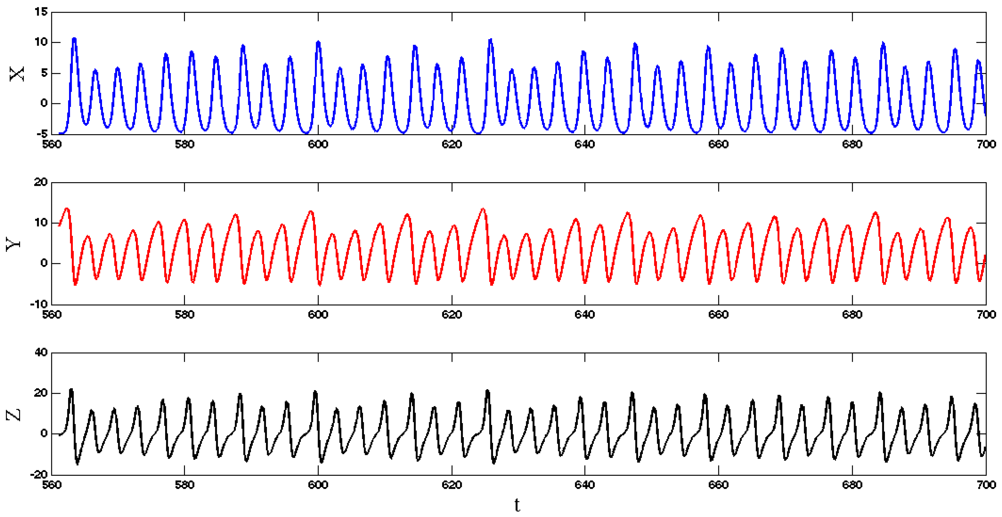
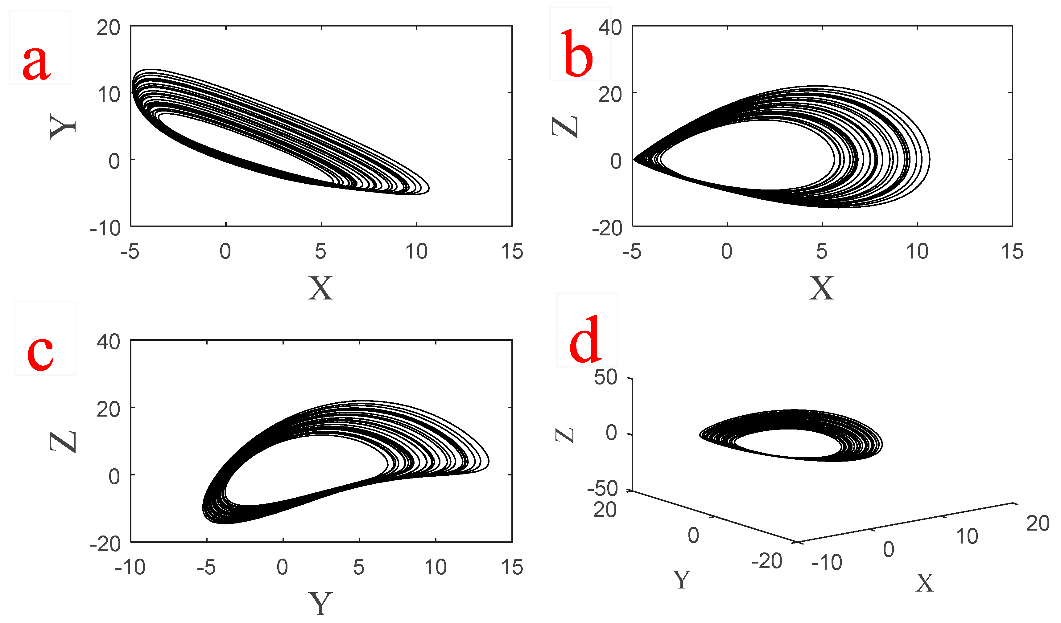
2. System Description

In this paper, we are going investigate the dynamic properties of the following system:
x ˙ = z y ˙ = x z z ˙ = 0.1 x + 5 y z + x y 0.3 x z + a
where parameter a = 1 . System (1) is a three-dimensional chaotic flow that can have a chaotic attractor. This system has been designed based on the method proposed in [41]. In the first step of investigating its dynamic properties, the equilibrium points of the system were calculated. By setting zero at the right hand side of this equation we obtain:
z = 0 x = 0 y = 1 5
Thus, the system has one equilibrium point in ( 0 ,   0.2 ,   0 ) . A stability analysis of this equilibrium point can be carried out using the following Jacobian matrix at the equilibrium:
J = [ 0 0 1 1 0 1 0.1 5 1 ]
By solving the equality det ( λ I J ) = 0 , the characteristic equation of System (1) is determined as follows:
λ 3 + λ 2 + 5.1 λ + 5 = 0
Solving Equation (4), we find that System (1) has three eigenvalues ( λ 1 = 0.9835 ,   λ 2 , 3 = 0.0082 ± 2.2547 i ) for the equilibrium ( 0 ,   0.2 ,   0 ) . Thus, it is a stable equilibrium point. Every other possible attractor of this system coexists with this stable equilibrium point. The system shows a chaotic attractor if we choose initial conditions ( x 0 , y 0 , z 0 ) = ( 5.4 ,   1.8 ,   3.3 ) . The chaotic attractor cannot be found using any equilibrium points of the system since the system has only one stable equilibrium point. Thus the strange attractor is hidden [27]. The time series of three states of System (1) for a = 1 are shown in Figure 1. Three projections of the chaotic attractor and its three-dimensional attractor are presented in Figure 2 and its Poincaré map is shown in Figure 3. In this plot, we use the peak values of x variable as the Poincaré map.

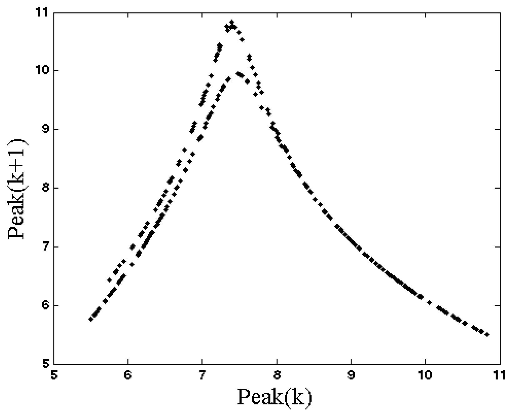
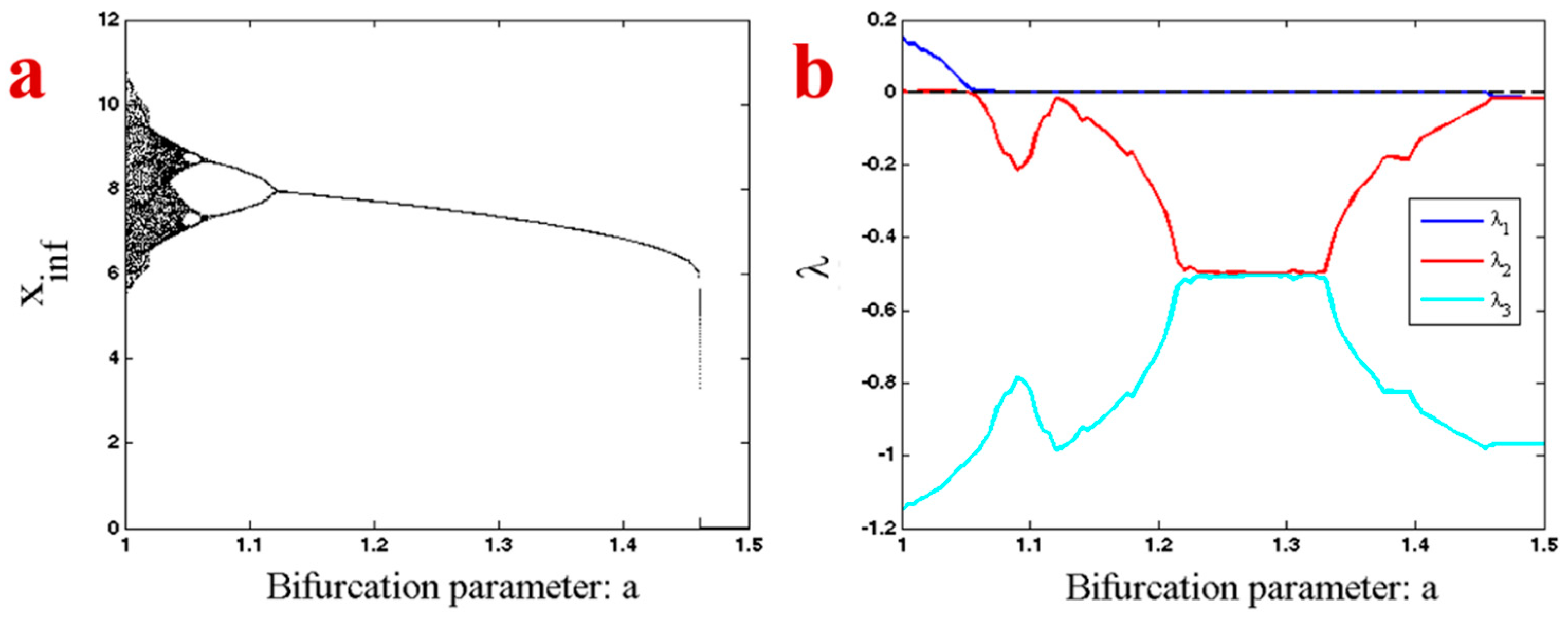
3. Bifurcation Analysis
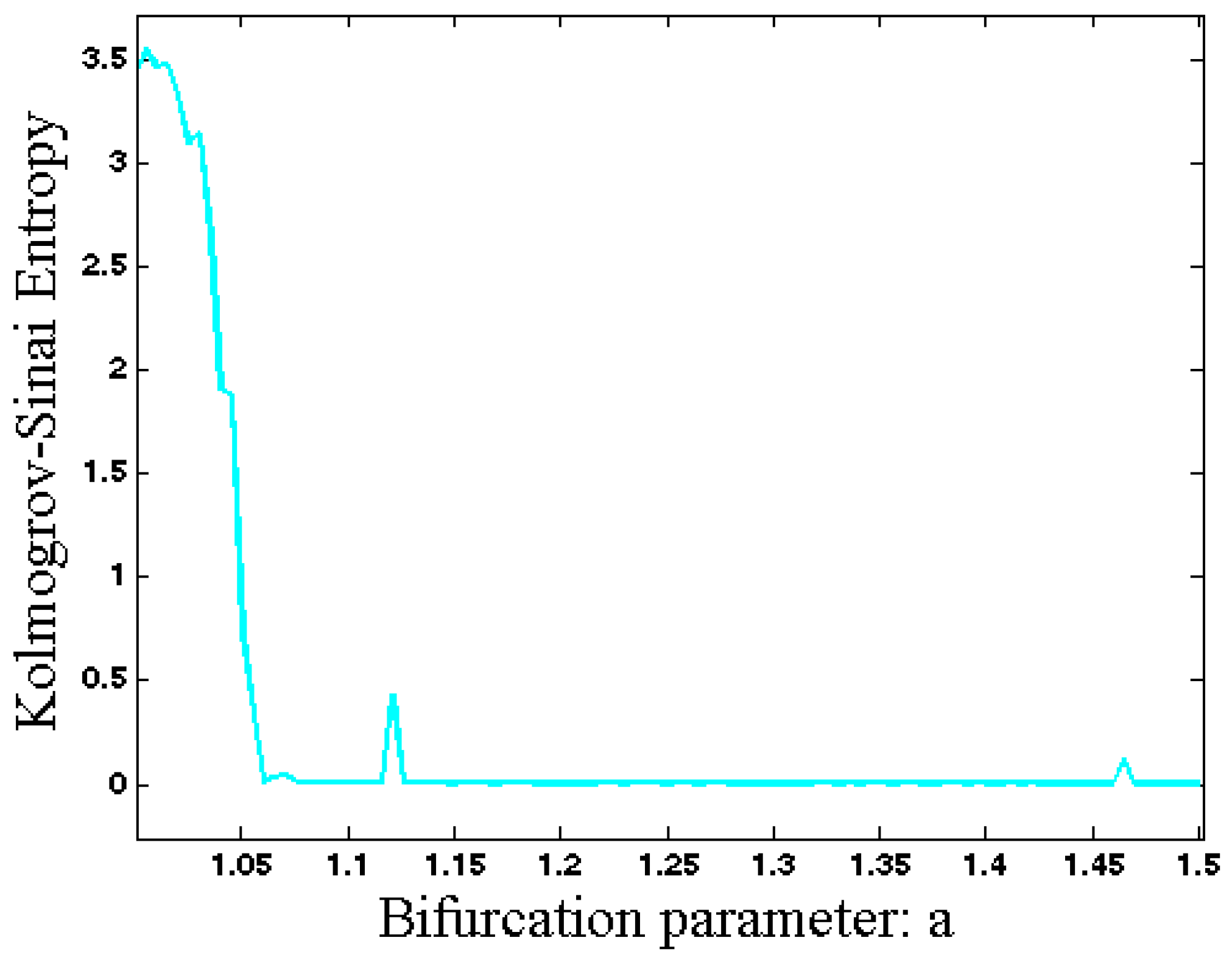
In order to show the different dynamic behaviors of System (1), its bifurcation diagram was investigated. Figure 4a shows a bifurcation diagram of the system with respect to the changing parameter a . The system has an inverse route of period doubling after its chaotic behavior. The dynamic of the system also suddenly changes in a = 1.46 from a stable limit cycle to a stable equilibrium. In other words, System (1) has a chaotic attractor in parameter a = 1 and initial conditions ( x 0 , y 0 , z 0 ) = ( 5.4 ,   1.8 ,   3.3 ) . The system also has a stable equilibrium point in ( 0 , a 5 , 0 ) = ( 0 , 1 5 , 0 ) . Thus, there are some initial conditions in the vicinity of this stable equilibrium that are attracted to it. In the bifurcation diagram of Figure 4, we used the initial conditions ( x 0 , y 0 , z 0 ) = ( 5.4 ,   1.8 ,   3.3 ) for parameter a = 1 and applied the forward continuation method for the higher values of parameter a . In other words, in the higher values of parameter a , we used initial conditions from the end of trajectory in the previous parameter with forward changing. Thus, the trajectory of the system traps into one attractor that is chaotic in parameter a = 1 and bifurcates with an inverse route of period doubling to chaos. In parameter a = 1.46 the previous attractor becomes unstable and the system jumps from a stable limit cycle to the stable equilibrium point ( 0 , a 5 , 0 ) . To be sure about the chaotic and other types of attractors of the system, it was necessary to calculate the Lyapunov exponents (Figure 4b). In the smaller values of the parameter a the system has a chaotic attractor (one positive, one zero, and one negative LE). It then shows the limit cycle, since its largest Lyapunov exponent is zero and the other two LEs are negative. After that, in the higher values of parameter a , the attractor changed to a stable equilibrium that has three negative Lyapunov exponents.

4. Entropy Analysis

Entropy is a measure of unpredictability. Shannon has proposed a formulation for calculating entropy [42]. Since chaotic attractors have an infinite number of states, another type of entropy is needed to calculate their unpredictability. This entropy is called Kolmogorov–Sinai ( H k s ) [40,43] and its formulation is shown in Equation (5).
H k s ( β [ ε ] ) = 1 τ m i n ( β [ ε ] ) τ ρ ( τ , β [ ε ] ) l o g ( 1 ρ ( τ , β [ ε ] ) )
It is defined using the first Poincaré recurrence times (FPRs) denoted by τ i . β is a D-dimensional box in the state space with side ε 1 where the FPRs are observed. ρ ( τ , β ) is the probability distribution of τ i . For a smooth chaotic system H k s is equal to the sum of all positive Lyapunov exponents [44,45]. The Kolmogorov–Sinai entropy of System (1) with respect to the changing parameter a is shown in Figure 5. Near a bifurcation point, the system’s state becomes slower. In other words, the transient time increases near a bifurcation point [46,47]. In order to use Kolmogorov–Sinai entropy to anticipate a bifurcation point, we calculated it without removing the transient time of the trajectory. If we remove the transient time, then the estimated Kolmogorov–Sinai entropy became zero in regular dynamics and it changed through variations in the final state of the system. By applying Kolmogorov–Sinai entropy to the system’s state without removing transient time, we were able to see complexity of transient parts as well as final state of the system. As Figure 5 shows, in small values of parameter a the system has a chaotic attractor and its unpredictability is high. By increasing parameter a , the system changes its dynamic to a regular dynamic and thus its entropy decreases. However, in the bifurcation points the system becomes slower and its transient time increases. That is the reason for the increasing entropy in the bifurcation points.

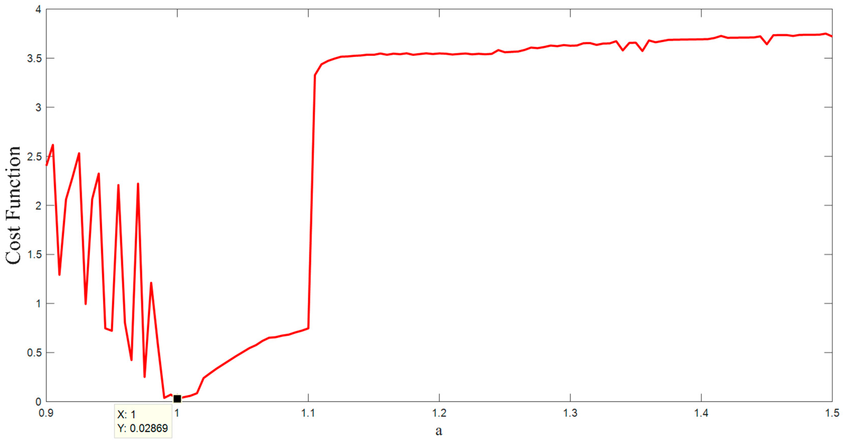
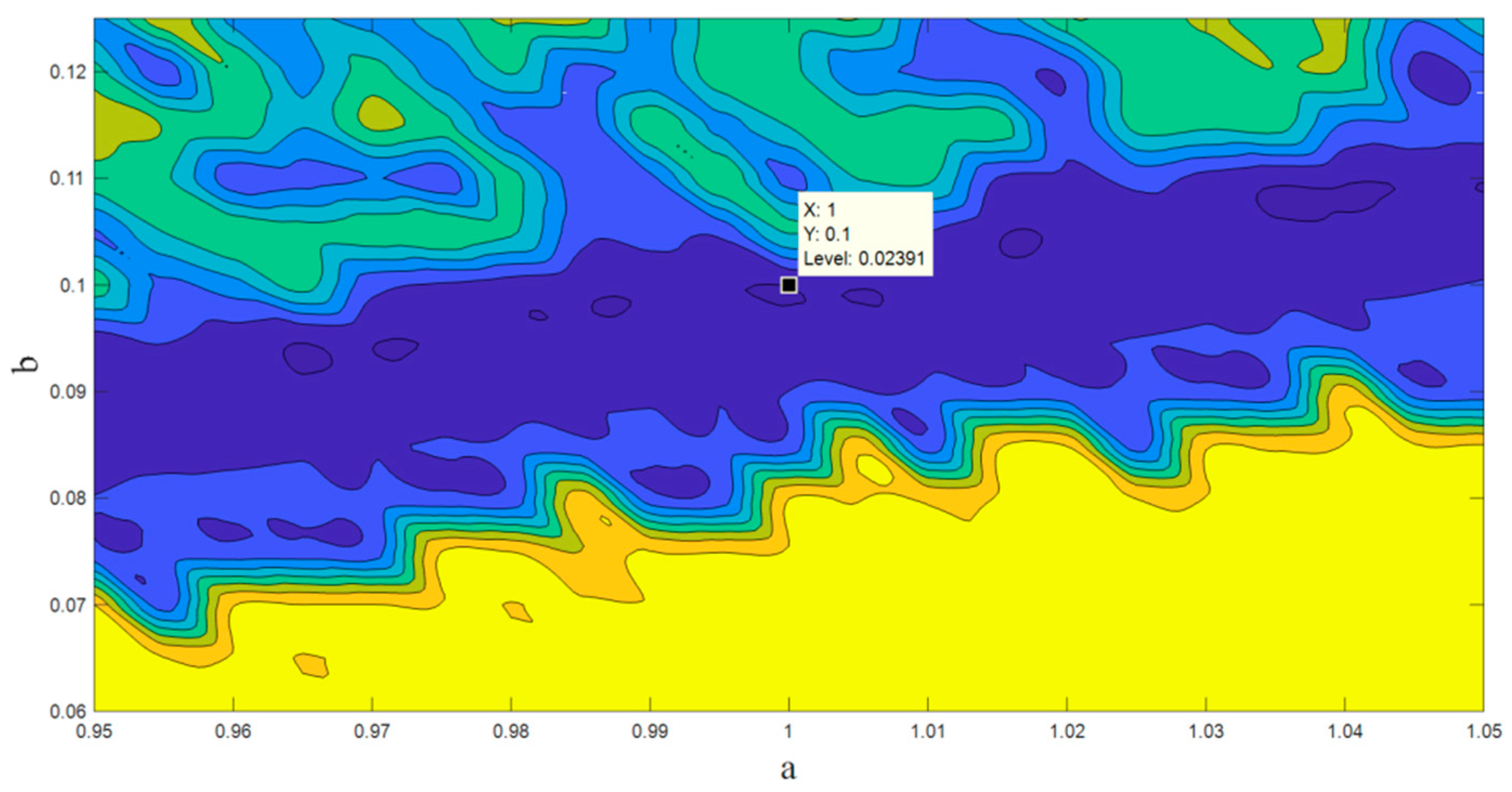
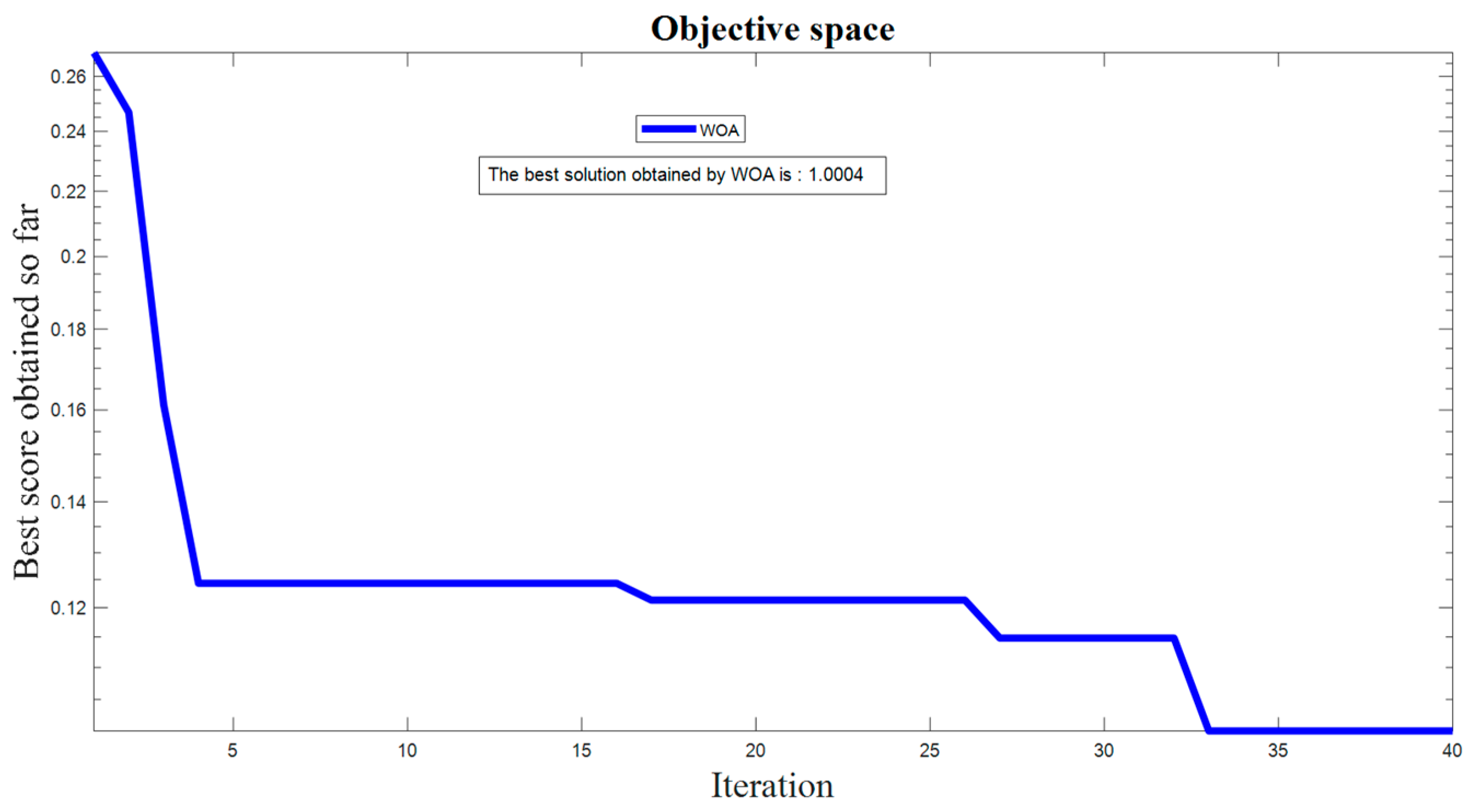
5. Parameter Estimation

There are various methods for parameter estimation in dynamic systems that are based on optimization methods [48,49,50]. The basis of these methods is a cost function associated with the differences between the time series obtained from a real system and the time series obtained from a known model with unknown parameters. However, these approaches are not appropriate for chaotic systems due to the butterfly effect [51,52,53]. Therefore an alternative method is proposed in [54,55]. This new method changes the analyzing domain of the chaotic system from time space to the state space. In the other words, this new model compares the topology and structure of the points in the state space. To this end, the algorithm searches the space of the parameter to find the most similar point from the model to the point of the data. Whenever the structure of the points in the state space gets close enough to the structure of the real data, the optimum parameter is found. For more complete details, see [55,56]. In this paper, we used this useful cost function along with WOA (whale optimization algorithm [57,58]) for the parameter estimation method. Figure 6 shows the result of the cost function with respect to changing the parameter a . As is shown in the figure, the global minimum is located exactly in the main parameter a = 1 . Figure 7 shows the result of the cost function with respect to changing the parameters a and b (consider b as the coefficient of x in the third equation of Equation (1)). As is shown in the figure, the global minimum is located in the main parameters a = 1   &   b = 0.1 .
One of the most efficient categories of the optimization methods is meta-heuristic methods, which cover a wide range of problems, especially in engineering applications [50,59,60,61]. Most of them are inspired by nature. Humpback whales’ hunting behavior in sea form the basis of the WOA (whale optimization algorithm) meta-heuristic algorithm [57,58]. The hunting behavior of Humpback whales, who encircle the recognized location of prey, has become the basis of the WOA algorithm. In this algorithm the target prey is the current best candidate or close to the optimum solution and the attacking strategy is a bubble-net strategy. By considering all these together, the WOA optimization method can be explained through three steps: Finding the prey, encircling the prey, and the bubble-net attacking behavior of humpback whales.
At first, the algorithm determines the best candidate solution. Then it updates the position of the other points in order to get closer to the best agent. The second step is about the attack strategy, which can be divided into two approaches. The first is a shrinking encircling mechanism and the other is a spiral updating position. For complete details see [57]. Figure 8 represents the result of the WOA for the 30 searching agents and 40 iterations.

6. Circuit Design

This section presents a circuit implementation for the three-dimensional flow (1) (see Figure 9). The circuit implementation in Figure 9 was constructed using six operational amplifiers ( U 1 U 6 ) and electronic elements [62,63,64,65,66]. We used TL084 operational amplifiers and AD633 analog multipliers. Taking the voltages of three operational amplifiers ( U 1 ,   U 2 ,   U 3 ) as X ,   Y ,   Z , it confirms that the circuit in Equation (6) corresponds to the flow (1):
X ˙ = 1 R 1 C 1 Z Y ˙ = 1 R 2 C 2 X 1 R 3 C 2 Z Z ˙ = 1 R 4 C 3 X + 1 R 5 C 3 Y 1 R 6 C 3 Z + 1 R 7 C 3 10 V X Y 1 R 8 C 3 10 V X Z 1 R 9 C 3 V a
where V a is a DC voltage source.
The circuit generates chaos as illustrated in Figure 10 for the following set of components: C 1 = C 2 = C 3 = 20   nF , R 1 = R 2 = R 3 = R 6 = R = 40   k Ω , R 4 = 400   k Ω , R 5 = 8   k Ω , R 7 = 1   k Ω , R 8 = 3.333   k Ω , R 9 = 160   k Ω , and V a = 1 V D C .

7. Conclusions

A new three-dimensional chaotic system with one stable equilibrium was proposed in this paper. A bifurcation analysis of the system showed an inverse period doubling route to chaos with respect to increasing parameter a . The unpredictability of its dynamic was discussed using Kolmogorov–Sinai entropy. Parameter estimation of the system was carried out and circuit implementation of the system confirmed its feasibility. It is noted that the real practical realization and real laboratory measurements of the circuit should be carried out. Therefore, practical results will be reported in our next works.

Author Contributions

Data curation, S.A.M., S.M., F.E.A. and T.H.; Formal analysis, F.E.A., T.H. and V.-T.P.; Investigation, T.K., S.A.M. and S.M.; Supervision, T.K.; Validation, T.K., S.A.M., S.M., F.E.A., T.H. and V.-T.P.; Writing—original draft, T.H. and V.-T.P.; Writing—review & editing, T.K., S.A.M., S.M., F.E.A., T.H. and V.-T.P.

Funding

TK was supported by the Polish National Science Centre, MAESTRO Programme-Project No. 2013/327 08/A/ST8/00/780.

Conflicts of Interest

The authors declare no conflict of interest.

References

  1. Lorenz, E.N. Deterministic nonperiodic flow. J. Atmos. Sci. 1963, 20, 130–141. [Google Scholar] [CrossRef]
  2. Chen, G.; Ueta, T. Yet another chaotic attractor. Int. J. Bifurc. Chaos 1999, 9, 1465–1466. [Google Scholar] [CrossRef]
  3. Jafari, S.; Sprott, J.; Golpayegani, S.M.R.H. Elementary quadratic chaotic flows with no equilibria. Phys. Lett. A 2013, 377, 699–702. [Google Scholar] [CrossRef]
  4. Wei, Z. Dynamical behaviors of a chaotic system with no equilibria. Phys. Lett. A 2011, 376, 102–108. [Google Scholar] [CrossRef]
  5. Lao, S.-K.; Shekofteh, Y.; Jafari, S.; Sprott, J.C. Cost function based on Gaussian mixture model for parameter estimation of a chaotic circuit with a hidden attractor. Int. J. Bifurc. Chaos 2014, 24, 1450010. [Google Scholar] [CrossRef]
  6. Wang, X.; Chen, G. A chaotic system with only one stable equilibrium. Commun. Nonlinear Sci. Numer. Simul. 2012, 17, 1264–1272. [Google Scholar] [CrossRef] [Green Version]
  7. Jafari, S.; Sprott, J. Simple chaotic flows with a line equilibrium. Chaos Solitons Fractals 2013, 57, 79–84. [Google Scholar] [CrossRef]
  8. Rajagopal, K.; Karthikeyan, A.; Srinivasan, A. Bifurcation and chaos in time delayed fractional order chaotic memfractor oscillator and its sliding mode synchronization with uncertainties. Chaos Solitons Fractals 2017, 103, 347–356. [Google Scholar] [CrossRef]
  9. Pham, V.-T.; Jafari, S.; Volos, C.; Vaidyanathan, S.; Kapitaniak, T. A chaotic system with infinite equilibria located on a piecewise linear curve. Opt.-Int. J. Light Electron Opt. 2016, 127, 9111–9117. [Google Scholar] [CrossRef]
  10. Barati, K.; Jafari, S.; Sprott, J.C.; Pham, V.-T. Simple Chaotic Flows with a Curve of Equilibria. Int. J. Bifurc. Chaos 2016, 26, 1630034. [Google Scholar] [CrossRef]
  11. Tolba, M.F.; Said, L.A.; Madian, A.H.; Radwan, A.G. FPGA implementation of fractional-order integrator and differentiator based on Grünwald Letnikov’s definition. In Proceedings of the 2017 29th International Conference on Microelectronics (ICM), Beirut, Lebanon, 10–13 December 2017; pp. 1–4. [Google Scholar]
  12. Kingni, S.T.; Pham, V.-T.; Jafari, S.; Kol, G.R.; Woafo, P. Three-Dimensional Chaotic Autonomous System with a Circular Equilibrium: Analysis, Circuit Implementation and Its Fractional-Order Form. Circuits Syst. Signal Process. 2016, 35, 1933–1948. [Google Scholar] [CrossRef]
  13. Ismail, S.M.; Said, L.A.; Rezk, A.A.; Radwan, A.G.; Madian, A.H.; Abu-Elyazeed, M.F.; Soliman, A.M. Generalized fractional logistic map encryption system based on FPGA. AEU-Int. J. Electron. Commun. 2017, 80, 114–126. [Google Scholar] [CrossRef]
  14. Jafari, S.; Sprott, J.C.; Molaie, M. A simple chaotic flow with a plane of equilibria. Int. J. Bifurc. Chaos 2016, 26, 1650098. [Google Scholar] [CrossRef]
  15. Bao, B.; Jiang, T.; Wang, G.; Jin, P.; Bao, H.; Chen, M. Two-memristor-based Chua’s hyperchaotic circuit with plane equilibrium and its extreme multistability. Nonlinear Dyn. 2017, 89, 1157–1171. [Google Scholar] [CrossRef]
  16. Jafari, S.; Sprott, J.C.; Pham, V.-T.; Volos, C.; Li, C. Simple chaotic 3D flows with surfaces of equilibria. Nonlinear Dyn. 2016, 86, 1349–1358. [Google Scholar] [CrossRef]
  17. Sun, K.; Sprott, J. A simple jerk system with piecewise exponential nonlinearity. Int. J. Nonlinear Sci. Numer. Simul. 2009, 10, 1443–1450. [Google Scholar] [CrossRef]
  18. Leonov, G.; Kuznetsov, N.; Vagaitsev, V. Localization of hidden Chua’s attractors. Phys. Lett. A 2011, 375, 2230–2233. [Google Scholar] [CrossRef]
  19. Leonov, G.; Kuznetsov, N.; Vagaitsev, V. Hidden attractor in smooth Chua systems. Phys. D Nonlinear Phenom. 2012, 241, 1482–1486. [Google Scholar] [CrossRef]
  20. Leonov, N.V.; Kuznetsov, G.A. Hidden attractors in dynamical systems. From hidden oscillations in Hilbert–Kolmogorov, Aizerman, Kalman problems to hidden chaotic attractor in Chua circuits. Int. J. Bifurc. Chaos 2013, 23, 1330002. [Google Scholar] [CrossRef]
  21. Leonov, G.; Kuznetsov, N.; Kiseleva, M.; Solovyeva, E.; Zaretskiy, A. Hidden oscillations in mathematical model of drilling system actuated by induction motor with a wound rotor. Nonlinear Dyn. 2014, 77, 277–288. [Google Scholar] [CrossRef]
  22. Leonov, G.; Kuznetsov, N.; Mokaev, T. Hidden attractor and homoclinic orbit in Lorenz-like system describing convective fluid motion in rotating cavity. Commun. Nonlinear Sci. Numer. Simul. 2015, 28, 166–174. [Google Scholar] [CrossRef] [Green Version]
  23. Leonov, G.A.; Kuznetsov, N.V.; Mokaev, T.N. Homoclinic orbits, and self-excited and hidden attractors in a Lorenz-like system describing convective fluid motion. Eur. Phys. J. Spec. Top. 2015, 224, 1421–1458. [Google Scholar] [CrossRef] [Green Version]
  24. Danca, M.-F.; Kuznetsov, N. Hidden chaotic sets in a Hopfield neural system. Chaos Solitons Fractals 2017, 103, 144–150. [Google Scholar] [CrossRef]
  25. Danca, M.-F.; Kuznetsov, N.; Chen, G. Unusual dynamics and hidden attractors of the Rabinovich–Fabrikant system. Nonlinear Dyn. 2017, 88, 791–805. [Google Scholar] [CrossRef]
  26. Kuznetsov, N.; Leonov, G.; Yuldashev, M.; Yuldashev, R. Hidden attractors in dynamical models of phase-locked loop circuits: Limitations of simulation in MATLAB and SPICE. Commun. Nonlinear Sci. Numer. Simul. 2017, 51, 39–49. [Google Scholar] [Green Version]
  27. Dudkowski, D.; Jafari, S.; Kapitaniak, T.; Kuznetsov, N.V.; Leonov, G.A.; Prasad, A. Hidden attractors in dynamical systems. Phys. Rep. 2016, 637, 1–50. [Google Scholar] [CrossRef]
  28. Hassard, B.D.; Kazarinoff, N.D.; Wan, Y.-H. Theory and Applications of Hopf Bifurcation; CUP Archive: Cambridge, UK, 1981; Volume 41. [Google Scholar]
  29. Stankevich, N.V.; Dvorak, A.; Astakhov, V.; Jaros, P.; Kapitaniak, M.; Perlikowski, P.; Kapitaniak, T. Chaos and Hyperchaos in Coupled Antiphase Driven Toda Oscillators. Regul. Chaotic Dyn. 2018, 23, 120–126. [Google Scholar] [CrossRef]
  30. Jaros, P.; Brezetsky, S.; Levchenko, R.; Dudkowski, D.; Kapitaniak, T.; Maistrenko, Y. Solitary states for coupled oscillators with inertia. Chaos Interdiscip. J. Nonlinear Sci. 2018, 28, 011103. [Google Scholar] [CrossRef] [PubMed] [Green Version]
  31. Kapitaniak, T.; Leonov, G.A. Multistability: Uncovering hidden attractors. Eur. Phys. J. Spec. Top. 2015, 224, 1405–1408. [Google Scholar] [CrossRef] [Green Version]
  32. Lai, Q.; Chen, S. Generating multiple chaotic attractors from Sprott B system. Int. J. Bifurc. Chaos 2016, 26, 1650177. [Google Scholar] [CrossRef]
  33. Lai, Q.; Wang, L. Chaos, bifurcation, coexisting attractors and circuit design of a three-dimensional continuous autonomous system. Opt.-Int. J. Light Electron Opt. 2016, 127, 5400–5406. [Google Scholar] [CrossRef]
  34. Kengne, J.; Njitacke, Z.; Fotsin, H. Dynamical analysis of a simple autonomous jerk system with multiple attractors. Nonlinear Dyn. 2016, 83, 751–765. [Google Scholar] [CrossRef]
  35. Ma, J.; Wu, F.; Ren, G.; Tang, J. A class of initials-dependent dynamical systems. Appl. Math. Comput. 2017, 298, 65–76. [Google Scholar] [CrossRef]
  36. Wei, Z.; Moroz, I.; Liu, A. Degenerate Hopf bifurcations, hidden attractors, and control in the extended Sprott E system with only one stable equilibrium. Turk. J. Math. 2014, 38, 672–687. [Google Scholar] [CrossRef] [Green Version]
  37. Wei, Z.; Zhang, W. Hidden hyperchaotic attractors in a modified Lorenz–Stenflo system with only one stable equilibrium. Int. J. Bifurc. Chaos 2014, 24, 1450127. [Google Scholar] [CrossRef]
  38. Hilborn, R.C. Chaos and Nonlinear Dynamics: An Introduction for Scientists and Engineers; Oxford University Press: Oxford, UK, 2000. [Google Scholar]
  39. Vaidyanathan, S.; Volos, C.; Pham, V.-T.; Madhavan, K.; Idowu, B.A. Adaptive backstepping control, synchronization and circuit simulation of a 3-D novel jerk chaotic system with two hyperbolic sinusoidal nonlinearities. Arch. Control Sci. 2014, 24, 375–403. [Google Scholar] [CrossRef] [Green Version]
  40. Tam, W.M.; Lau, F.C.; Chi, K.T. Digital Communications with Chaos: Multiple Access Techniques and Performance; Elsevier: New York, NY, USA, 2010. [Google Scholar]
  41. Molaie, M.; Jafari, S.; Sprott, J.C.; Golpayegani, S.M.R.H. Simple chaotic flows with one stable equilibrium. Int. J. Bifurc. Chaos 2013, 23, 1350188. [Google Scholar] [CrossRef]
  42. Kant, N.A.; Dar, M.R.; Khanday, F.A.; Psychalinos, C. Ultra-low-Voltage Integrable Electronic Realization of Integer-and Fractional-Order Liao’s Chaotic Delayed Neuron Model. Circuits Syst. Signal Process. 2017, 36, 4844–4868. [Google Scholar] [CrossRef]
  43. Tsirimokou, G.; Psychalinos, C.; Elwakil, A.S.; Salama, K.N. Electronically tunable fully integrated fractional-order resonator. IEEE Trans. Circuits Syst. II Express Br. 2018, 65, 166–170. [Google Scholar] [CrossRef]
  44. Bertsias, P.; Psychalinos, C.; Radwan, A.G.; Elwakil, A.S. High-Frequency Capacitorless Fractional-Order CPE and FI Emulator. Circuits Syst. Signal Process. 2017, 37, 2694–2713. [Google Scholar] [CrossRef]
  45. Tang, Y.X.; Khalaf, A.J.M.; Rajagopal, K.; Pham, V.T.; Jafari, S.; Tian, Y. A new nonlinear oscillator with infinite number of coexisting hidden and self-excited attractors. Chin. Phys. B 2018, 27, 040502. [Google Scholar] [CrossRef]
  46. Alghassab, M.; Mahmoud, A.; Zohdy, M.A. Nonlinear Control of Chaotic Forced Duffing and Van der Pol Oscillators. Int. J. Mod. Nonlinear Theory Appl. 2017, 6, 26. [Google Scholar] [CrossRef]
  47. Njah, A. Synchronization via active control of parametrically and externally excited Φ6 Van der Pol and Duffing oscillators and application to secure communications. J. Vib. Control 2011, 17, 493–504. [Google Scholar] [CrossRef]
  48. He, Q.; Wang, L.; Liu, B. Parameter estimation for chaotic systems by particle swarm optimization. Chaos Solitons Fractals 2007, 34, 654–661. [Google Scholar] [CrossRef]
  49. Tang, Y.; Guan, X. Parameter estimation for time-delay chaotic system by particle swarm optimization. Chaos Solitons Fractals 2009, 40, 1391–1398. [Google Scholar] [CrossRef]
  50. Wang, L.; Xu, Y. An effective hybrid biogeography-based optimization algorithm for parameter estimation of chaotic systems. Expert Syst. Appl. 2011, 38, 15103–15109. [Google Scholar] [CrossRef]
  51. Jafari, S.; Hashemi Golpayegani, S.M.R.; Jafari, A.H.; Gharibzadeh, S. Some remarks on chaotic systems. Int. J. Gen. Syst. 2012, 41, 329–330. [Google Scholar] [CrossRef]
  52. Jafari, S.; Hashemi Golpayegani, S.M.R.; Daliri, A. Parameters identification of chaotic systems by quantum-behaved particle swarm optimization. Int. J. Comput. Math. 2009, 86, 2225–2235, Comment on Int. J. Comput. Math. 2013, 90, 903–905. [Google Scholar]
  53. Jafari, S.; Hashemi Golpayegani, S.M.R.; Rasoulzadeh Darabad, M. Parameter identification and synchronization of fractional-order chaotic systems. Commun. Nonlinear Sci. Numer. Simul. 2012, 17, 305–316, Comment on Commun. Nonlinear Sci. Numer. Simul. 2013, 18, 811–814. [Google Scholar]
  54. Shekofteh, Y.; Jafari, S.; Sprott, J.C.; Hashemi Golpayegani, S.M.R.; Almasganj, F. A gaussian mixture model based cost function for parameter estimation of chaotic biological systems. Commun. Nonlinear Sci. Numer. Simul. 2015, 20, 469–481. [Google Scholar] [CrossRef]
  55. Jafari, S.; Sprott, J.C.; Pham, V.-T.; Hashemi Golpayegani, S.M.R.; Jafari, A.H. A New Cost Function for Parameter Estimation of Chaotic Systems Using Return Maps as Fingerprints. Int. J. Bifurc. Chaos 2014, 24, 1450134. [Google Scholar] [CrossRef]
  56. Kingni, S.T.; Jafari, S.; Simo, H.; Woafo, P. Three-dimensional chaotic autonomous system with only one stable equilibrium: Analysis, circuit design, parameter estimation, control, synchronization and its fractional-order form. Eur. Phys. J. Plus 2014, 129, 76. [Google Scholar] [CrossRef]
  57. Wang, Z.; Abdolmohammadi, H.R.; Alsaadi, F.E.; Hayat, T.; Pham, V.-T. A new oscillator with infinite coexisting asymmetric attractors. Chaos Solitons Fractals 2018, 110, 252–258. [Google Scholar] [CrossRef]
  58. Hu, X.; Liu, C.; Liu, L.; Ni, J.; Yao, Y. Chaotic dynamics in a neural network under electromagnetic radiation. Nonlinear Dyn. 2018, 91, 1541–1554. [Google Scholar] [CrossRef]
  59. Hu, X.; Liu, C.; Liu, L.; Ni, J.; Li, S. An electronic implementation for Morris–Lecar neuron model. Nonlinear Dyn. 2016, 84, 2317–2332. [Google Scholar] [CrossRef]
  60. Lee, K.S.; Geem, Z.W. A new meta-heuristic algorithm for continuous engineering optimization: Harmony search theorypractice. Comput. Methods Appl. Mech. Eng. 2005, 194, 3902–3933. [Google Scholar] [CrossRef]
  61. Hu, X.; Liu, C.; Liu, L.; Yao, Y.; Zheng, G. Multi-scroll hidden attractors and multi-wing hidden attractors in a 5-dimensional memristive system. Chin. Phys. B 2017, 26, 110502. [Google Scholar] [CrossRef]
  62. Hu, X.; Liu, C.; Liu, L.; Ni, J.; Li, S. Multi-scroll hidden attractors in improved Sprott A system. Nonlinear Dyn. 2016, 86, 1725–1734. [Google Scholar] [CrossRef]
  63. Majhi, S.; Perc, M.; Ghosh, D. Chimera states in a multilayer network of coupled and uncoupled neurons. Chaos Interdiscip. J. Nonlinear Sci. 2017, 27, 073109. [Google Scholar] [CrossRef] [PubMed] [Green Version]
  64. Namazi, H.; Daneshi, A.; Azarnoush, H.; Jafari, S.; Towhidkhah, F. Fractal based analysis of the influence of auditory stimuli on eye movements. Fractals 2018, 26, 1850040. [Google Scholar] [CrossRef]
  65. Gosak, M.; Stožer, A.; Markovič, R.; Dolenšek, J.; Marhl, M.; Slak Rupnik, M.; Perc, M. The relationship between node degree and dissipation rate in networks of diffusively coupled oscillators and its significance for pancreatic beta cells. Chaos Interdiscip. J. Nonlinear Sci. 2015, 25, 073115. [Google Scholar] [CrossRef] [PubMed]
  66. Smirnova, R.; Zakrzhevsky, M.; Schukin, I. Global analysis of the nonlinear Duffing-van der Pol type equation by a bifurcation theory and complete bifurcation groups method. Vibroeng. Procedia 2014, 3, 139–143. [Google Scholar]
Figure 1. Time series of System (1) with parameter a = 1 and initial conditions ( x 0 , y 0 , z 0 ) = ( 5.4 ,   1.8 ,   3.3 ) .
Entropy 20 00670 g001
Figure 2. Three projections of the chaotic attractor of System (1) with parameter a = 1 and initial conditions ( x 0 , y 0 , z 0 ) = ( 5.4 ,   1.8 ,   3.3 ) in (a) X-Y plane. (b) X-Z plane. (c) Y-Z plane and (d) 3-D chaotic attractor.
Entropy 20 00670 g002
Figure 3. Poincaré map (peaks of x variable) of System (1) with parameter a = 1 and initial conditions ( x 0 , y 0 , z 0 ) = ( 5.4 ,   1.8 ,   3.3 ) .
Entropy 20 00670 g003
Figure 4. (a) Bifurcation diagram of System (1) with respect to the changing parameter a in the interval [1, 1.5] and forward continuation. (b) Lyapunov exponents of System (1) with respect to the changing parameter a in the interval [1, 1.5] and forward continuation.
Entropy 20 00670 g004
Figure 5. Kolmogorov–Sinai entropy of System (1) with respect to changing parameter a.
Entropy 20 00670 g005
Figure 6. The value of the cost function with respect to changing the parameter a.
Entropy 20 00670 g006
Figure 7. The value of the cost function with respect to changing the parameter a & b.
Entropy 20 00670 g007
Figure 8. The result of WOA for the 30 searching agents and 40 iterations.
Entropy 20 00670 g008
Figure 9. The circuit constructed by six operational amplifiers ( U 1 U 6 ) and electronic elements.
Entropy 20 00670 g009
Figure 10. Generated attractors in PSpice of the circuit: (a) X-Y plane, (b) X-Z plane, (c) Y-Z plane.
Entropy 20 00670 g010

