1. Introduction
By the Boltzmann–Einstein relation, the free energy of a system is inherently related to the fluctuations of an underlying microscopic particle system. In this sense, two systems with the same macroscopic behaviour can be driven by completely different free energies, if their corresponding microscopic systems are different. Therefore, one of the main objectives of (equilibrium) statistical mechanics is to derive the “physically correct” macroscopic free energy from fluctuations in microscopic systems. A similar principle can be applied to systems that evolve over time, where dynamic fluctuations may lead to a gradient flow, driven by the free energy. For stochastically reversible systems and close to equilibrium this is the classic Onsager–Machlup theory [
1,
2]. Such relations are known to hold for many reversible dynamics, not necessarily close to equilibrium [
3]. More recently, it was shown that microscopic reversibility always implies the emergence of a macroscopic gradient flow [
4], but in this generality one needs to allow for so-called generalised gradient flows. In brief, a generalised gradient structure (GGS) is defined by a possibly non-linear relation between velocities and affinities. Although there exist non-reversible models that lead to macroscopic gradient flows [
5], these are considered non-typical; so in order to understand systems with non-reversible microscopic fluctuations, one needs to look for even further (thermodynamically consistent) generalisations of a gradient flow.
One such generalisation is a class of equations called GENERIC [
6]. These equations can be seen as a coupling between a gradient flow of some non-increasing free energy (or non-decreasing entropy) and a Hamiltonian system of some conserved energy. One assumes that the two structures are in a sense orthogonal to each other, which then guarantees that also for the coupled evolution, the free energy is non-decreasing and the Hamiltonian energy is conserved. We explain this concept in more details in
Section 3.3 and
Section 4.2.
The first GENERIC structure that was derived from dynamical large deviations can be found in [
7]. In order to pursue a similar procedure in a general setting, one again needs to allow for non-linear relations, just like generalised gradient flows. One is thus lead to study generalised GENERIC structures (GGEN) [
8]. In a recent work, necessary and sufficient conditions were found under which microscopic fluctuations induce such a GGEN structure [
9,
10].
Naturally, many systems do not satisfy those conditions nor do they have a GGEN structure. Therefore there is a need for even more general structures that can still be given a meaningful thermodynamic interpretation. At this point we place ourselves in the context of Macroscopic Fluctuation Theory (MFT) [
11]. Central to MFT is the idea that more thermodynamic properties of non-equilibrium fluctuations can be derived if, in addition to macroscopic state variables, the corresponding fluxes are taken into account. In general, fluxes hold more information than state variables due to the possible occurrence of “divergence-free” fluxes that do not alter the states.
One way in which this extra information can be exploited is to extract a generalisation of a GGS, where the affinity/driving force may no longer be the gradient of some free energy [
12,
13,
14,
15].
Another way to exploit the flux fluctuations, which is pursued in this paper, is to extract GGS/GGEN structures in a larger “flux space”. The heuristics behind this is that a GGS/GGEN, even in flux space, can be interpreted as a free energy balance. If there would be work done that results in a divergence-free flux, then one might expect an gap in the energy balance, so that such systems can not induce a GGS or GGEN. Could it be possible for such a system to have a GGS/GGEN structure in the flux space, when it fails to have a GGS/GGEN structure in the state space? The main point of this paper is that this is generally impossible. We will see in Theorem 3 that if the fluctuations induce a GGS or GGEN in the space of fluxes, this is, up to physical conditions, equivalent to the fluctuations inducing a GGS or GGEN in the state space.
Our leading example and main application will be that of a (non-spatial) isothermal chemical reaction network, as studied in [
16]. In
Section 2 we recall the main arguments from that paper, applied to concentrations undergoing reactions. In
Section 3 we expand these ideas and show how they can be applied to reaction fluxes. It turns out that reactions that occur on a faster time scale may give rise to a GGEN Hamiltonian part. Based on this example, we then develop an abstract theory about induced GGSs and GGENs in flux space, in
Section 4. To show the generality of these principles, we then show in
Section 5 how the theory applies to transport fluxes in a diffusing particles model, and in
Section 6 we combine the arguments from
Section 3 and
Section 6 to derive results for transport and reaction fluxes in a simple reaction-diffusion model.
2. Leading Example 1: Chemical Reactions
In this section we explain the main concepts, mostly by reiterating the arguments of [
4] and [
16]. In particular, we argue that large deviations/fluctuations provide a “physically correct” GGS for the evolution of concentrations undergoing chemical reactions.
Consider a network of isothermal chemical reactions, for example:
We denote the set of species by
(in this example
) and the set of reactions by
; for each reaction
r we consider a forward and backward reaction (so that here
consists of one element). The stoichiometric coefficients are denoted by
for the forward reactants (here
) and
for the forward products (here
), which yields the state change matrix
. The evolution of the concentrations
is then described by the
Reaction Rate Equation,
with concentration-dependent reaction rates
.
Typically (and often in this paper), the reaction rates will be of the form
for some constants
, using the notation
. In that case the network is said to be of
mass-action kinetics. For more background on chemical reaction networks we refer to the survey [
17]. More details about the fluctuations and induced GGSs for chemical reaction networks can be found in [
16]; for completeness we shall recall these results in this section.
To notationally stress the similarity and differences between different concepts throughout this paper, we shall always denote net quantities by a bar (), and we distinguish functionals on state space from functionals on flux space by a hat (). In this section we study concentrations only, which we consider to be states.
2.1. Reacting Particle System
A classical microscopic particle system underlying the evolution (
1) is the following [
18]. Let
V be a large, well-mixed volume that contains, at time
t, a total number
of particles of species
,
. A reaction
r occurs randomly with some propensities (jump rates)
. Whenever a forward reaction
r occurs,
particles are removed and
particles are created, and vice versa for a backward reaction. Hence each reaction requires a cumbersome relabelling of particles
. It is therefore more practical to work directly with the (particles per volume) concentration
. This quantity will also play the role of the macroscopic state variable. Whenever a forward or backward reaction
r takes place, the concentration can now be simply updated by a jump
. Then the
-dimensional vector
is a Markov jump process, which satisfies the master equation
It will be beneficial to work with the corresponding generator, which is the adjoint of the right-hand side of the master equation, with respect to the dual pairing
with an arbitrary test function:
The propensities that are usually used in the so-called chemical master Equation [
17] are derived from combinatoric considerations, and yield the mass-action kinetics in the limit [
16,
18]:
using the notation
and
.
2.2. Equilibrium: Limit, Large Deviations and Free Energy
We will from now on (throughout this section) assume that the reaction network is of mass-action kinetics (
2), and chemically detailed balanced, i.e., there exists a
for which
Naturally,
is an equilibrium under the deterministic evolution (
1). It should be stressed that, given an initial concentration
, both the deterministic evolution and the stochastic model is confined to the “stoichiometric compatibility class”
. Therefore, it is not clear whether this equilibrium
lies within the compatibility class that corresponds to the initial concentration. However, if there exists a detailed balanced concentration
, then there exists a unique detailed balanced concentration within each such class, see [
17] and the references therein. Without loss of generality, we can therefore implicitly assume that the detailed balanced equilibrium is unique, and lies within the correct compatibility class.
Under Assumption (
5), the invariant distribution of the stochastic model is known to be [
17]:
Letting
, this invariant distribution concentrates on the equilibrium state:
One can then extract the free energy by considering the corresponding large deviations, i.e., the exponential rate which with
converges to zero. Indeed, by Stirling’s formula,
Such limit is known as a large-deviation principle; the function on the right characterises the stochastic cost of microscopic fluctuations. If the reaction rates are related to an internal energy via Arrhenius’ law, then the expression
is really the Helmholtz free energy, apart from a normalisation term and a constant scaling, as explained in more detail in (Section 2.2 & 2.3, [
16]).
2.3. Dynamics: Limit and Large Deviations
Observe that in the microscopic model, the process speeds up as
V increases with order
V while the jump sizes are of size
. Therefore by (
4), as
the generator
converges to the limit generator,
Since this generator depends on the test function
f through
only, we can make the ansatz that the limit process is deterministic
, for some curve
. Plugging this into the definition of the generator yields:
As this relation holds for any test function
f, we see that the ansatz was justified if the postulated curve
satisfies the Reaction Rate Equation (
1). Hence the stochastic process
converges (pathwise in probability) to the deterministic solution
of the Reaction Rate Equation.
Similar to the calculation of the fluctuations of the equilibrium (
6), we can study the large deviations of the path probabilities
; this is known as a dynamic large-deviation principle. These dynamical fluctuations can be formally calculated with the framework of [
19]. To this aim we study the non-linear generator:
As before, the limit depends on the test function through
only, which is consistent with the fact that the limit is deterministic. We then define, by a slight abuse of notation,
The dynamic large-deviation principle now states that
The rigorous definition of the large-deviation principle, the heuristics behind this method, and the rigorous proof of this statement is all beyond the scope of this paper. For the precise details we refer to [
19], and for the rigorous proof for this particular system (by more classical methods) to [
20,
21,
22]. For the sake of brevity, we assume that the randomness in the initial condition is sufficiently small (e.g., deterministic) so that we do not obtain initial fluctuations.
Remark 1. The function (8) is implicitly defined as a supremum; although the supremum can be calculated explicitly, this leads to very cumbersome expressions. However, it does have a dual formulation in terms of a minimisation problem:where , similar to (6). Although the relative entropy h appears in both expressions, they should not be confused: is an equilibrium rate whereas is a dynamic quantity. We shall see later on that the latter can be directly (without the infimum) be interpreted as a large-deviation rate, where the variable j is a reaction flux. 2.4. GGS, Energy Balance, and Relation with Fluctuations
The (naive) aim is to rewrite the macroscopic equation as a gradient flow of some free energy
:
where
is some linear symmetric, positive definite (linear response) operator that maps thermodynamic forces to velocities. Mathematically, this operator can be interpreted as the inverse of the metric tensor of some manifold, so that the right-hand side is the gradient on this manifold.
Clearly, (
10) is equivalent to requiring
if we set
and
. Integrated over a time interval
, this reads
The last two terms describe the free energy loss (or entropy production), and the first two terms describe the dissipation; as such this equation represents a free energy balance. (For a linear gradient flow (
10),
; hence the dissipation can be seen as a kinetic energy. This is however no longer true for general GGSs).
Observe that this expression is always non-negative, and is 0 exactly on the gradient flow (
10). Moreover, we see that this expression has the same dimension as
, the free energy; it is indeed the free energy cost to deviate from the macroscopic dynamics. This interpretation shows that this cost should be equal to the cost
of microscopic fluctuations (
9).
This is in many cases, and particularly in this case of chemical reactions, impossible. Since the large-deviation function (
8) is non-quadratic, one should allow for non-quadratic dissipation terms. We therefore replace the two squared norms by a pair of dual
dissipation potentials:
where, as in the quadratic case, the potentials are convex duals of each other, i.e.,
and
. Moreover, we assume that
and
are both non-negative; from (12) we then see that the free energy
is non-increasing on the flow.
The right-hand side of (12) is always non-negative, since
by definition of the convex dual. Therefore, the right-hand side of (12) can only be 0 if
is minimal in the right-hand side. By differentiation we then get that (12) implies:
We call such equation a
generalised gradient flow, and the underlying structure
a
generalised gradient structure (GGS). Note that the generalisation with respect to (
10) lies in the fact that we allow for a non-linear relation between forces and velocities. We moreover say that a gradient structure is
induced by a cost function
whenever
.
In
Section 4 we will recall the relation between fluctuation costs and GGSs, as described in [
4]. Applied to the current setting of chemical reactions, we reiterate the following result from [
16]. If we again assume mass-action kinetics (
2) and chemical detailed balance (
5), then there exists a unique GGS
induced by the large-deviation cost
from (
8), where
with
. Since
appears as a sum, the expression for
becomes a so-called inf-convolution where all reactions are strongly intertwined. For more details on these inf-convolutions and the factor
in front of the free energy, we again refer to (Section 3.4, [
16]).
4. General Theory
Following the examples of
Section 2 and
Section 3, we now develop a more abstract framework to study the relation between energy-driven structures in flux and in state space.
4.1. Geometry and Notation
Throughout this section we assume to be given:
A differentiable manifold (“flux space”), where tangents are denoted by and cotangents by . Note that we distinguish between tangents and cotangents; we write the dual pairing between them as or simply ;
A differentiable manifold (“state space”), where tangents are denoted by and cotangents by ;
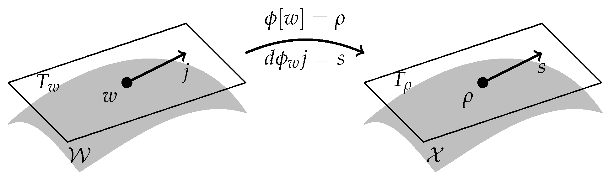
A surjective differentiable operator
with bounded linear differential
and adjoint differential
. This defines an abstract continuity equation
, or in differentiated form
, see
Figure 1. Contrary to
Section 2 and
Section 3, the second continuity equation may now also depend on
w. In practice, the continuity mapping
depends on the initial state
, which we assume to be fixed.
An L-function on flux space (see below for the definition of L-functions). This function could be a dynamic large-deviation cost function corresponding to random fluxes in some microscopic system, but throughout this section it could also be a more general expression.
An L-function
on state space, related to the flux space L-function via
This relation is again inspired by large-deviation theory, where such relation holds due to the contraction principle (Theorem 4.2.1, [
23]).
Corresponding to the L-functions are their convex duals with respect to their second variable, i.e.,
and
with
We express assumptions in terms of these duals, since in practice they are often more explicitly given than their corresponding L-functions.
Recall that in the previous section we saw that
depends on
w through
only. This condition becomes slightly more complicated in non-flat spaces, for a number of reasons. Firstly, the flux
j can not be kept fixed while changing
w, unless one has a path-independent notion of parallel transport, i.e., the space is flat. Secondly, even if
would not depend on
w, this dependence could re-enter through the continuity equation in the infimum
. Therefore, the condition that we need is that
for all
. It is easily seen that this condition is equivalent to the following flux invariance:
All manifolds and functionals are assumed to be sufficiently differentiable wherever needed. For a (differentiable) functional (and similarly on flux space) we write for the derivative, in the sense that on a curve .
4.2. Definitions
We now define the notions of L-functions, dissipation potentials, GGS, pGGEN, Poisson operators and GGEN on flux space; the same concepts on state space are defined analogously. Naturally all notions are compatible with the exposition from
Section 2 and
Section 3.
Definition 1. We say is an L-function whenever for all :
- (i)
is convex;
- (ii)
for some unique vector field .
Since is non-negative, the second condition simply means that should have a unique minimiser; this minimiser corresponds to an evolution equation of the type . Indeed, since is a minimiser, it will generally satisfy the implicit equation . Due to the convexity, is also the convex dual of .
Central to GGS, pGGEN and GGEN is the notion of dissipation potentials:
Definition 2. A function is called a dissipation potential whenever for all :
- (i)
is convex;
- (ii)
;
If these conditions hold, then the same conditions hold for the (pre-)dual dissipation potential We also say that is a dissipation potential pair whenever Ψ is a dissipation potential.
Definition 3. A generalised gradient system
(GGS) is a triple , where is a differentiable manifold, and is a dissipation potential. We say that an L-function induces a GGS whenever for all : As explained in
Section 3.3, by extending a GGS with an orthogonal drift one arrives at
Definition 4 ([
10])
. A Generalised pre-GENERIC system
(pGGEN) is a quadruple , where is a differentiable manifold, Ψ is a dissipation potential, , and is a vector field such that: We say that an L-function induces a pGGEN whenever for all : Finally, if the drift has the form of an Hamiltonian system that behaves more or less independently of the GGS part we arrive at a Generalised GENERIC system. In order to define this we first define:
Definition 5. A linear operator is called a Poisson structure if it satisfies the Jacobi identityfor all , where ; Jacobi’s identity implies skew symmetry, i.e., for all , ; in particular one has . Finally,
Definition 6 (Section 2.5, [
8])
. A generalised GENERIC system
(GGEN) is a quintuple , where is a differentiable manifold, Ψ is a dissipation potential, , is a Poisson structure, and the two non-interaction conditions are satisfied: We say that an L-function induces a GGEN whenever for all : Remark 2. If a GGS, pGGEN or GGEN is given on a manifold , and the dissipation potentials are quadratic (as explained in Section 2.4), then one can use the positive definite operator to define a new manifold, and redefine everything on this manifold. This allows to study the structures from a more geometric point of view. 4.3. From L-Functions to GGS, pGGEN and GGEN
We now recall some of the main results from [
4,
10], that give necessary and sufficient conditions for an L-function to induce a GGS or pGGEN. A similar result for GGEN does not exist, since an L-function does not uniquely determine a Poisson operator and Hamiltonian energy. However, from a pGGEN one can always construct a GGEN (in a non-unique way); for that result we refer the reader to (Section 4, [
10]).
Again, the following results are described, but not restricted to flux space.
Theorem 1 (Proposition 2.1 & Theorem 2.1, [
4])
. Let be an L-function with convex dual , and let be given. Then the following statements are equivalent: - (i)
induces a GGS for some dissipation potential Ψ,
- (ii)
for some dissipation potential ,
- (iii)
(34)
- (iv)
(35)
In that case (and indirectly Ψ) is uniquely determined by From condition (35) we see that , if it exists, is uniquely given up to constants. Note in particular that conditions (34) and (35) do not involve .
Theorem 2 (Theorem 3.6, [
10])
. Let be an L-function with convex dual , and let and a vector field be given for which . Then the following statements are equivalent: - (i)
induces a pGGEN for some dissipation potential Ψ,
- (ii)
(37)
- (iii)
,
- (iv)
(38)
In that case is uniquely determined by From condition (37) we see that must consist of a convex part and a linear part , so that the drift b is a priori and uniquely fixed by . Therefore is again uniquely fixed by condition (38). This is different from the GENERIC setting; uniquely defines and vice versa, but the whole quintuple may not be unique. However, one can still state a GENERIC analogue of Theorems 1 and 2 as follows:
Proposition 1. Let be an L-function with convex dual , and let a Poisson structure and energies be given such that the non-interaction condition holds. Then the following statements are equivalent:
- (i)
induces a GGEN for some dissipation potential Ψ,
- (ii)
and - (iii)
and (41)
In that case is uniquely determined by Proof. By Lemma 1 (see below), we can apply Theorem 1 to the shifted L-function
and back. This yields the three equivalences, apart from the other non-interaction condition (
31). From the explicit formula (
43) one finds that the missing non-interaction condition is equivalent to (
40) and to (
42). ☐
The previous proof made use of the following lemma:
Lemma 1. Let be a Poisson operator, be energies and Ψ be a dissipation potential such that the non-interaction conditions (31) and (32) hold. An L-function induces an GGEN if and only if the shifted L-function induces the GGS . Proof. Because of the non-interaction condition (
32), the shift transforms relation (
33) into (
30), and analogously for the other direction. ☐
4.4. Relation between Structures in Flux and State Space
We now consider L-functions and on flux and state space, and study how their induced structures are related.
Proposition 2. Assume that an L-function induces a pGGEN where andfor some . Then the L-function given by (
27)
induces a GGS for some dissipation potential . Proof. Since
and
, we can rewrite
and because
is a dissipation potential pair, clearly
This is equivalent to , which by Theorem 1 implies that induces a GGS for some . ☐
In the above proposition, also depends on w through only, which is a very physical assumption. It does imply however, that the equilibria of the flux gradient system can only be unique up to the kernel of ; this kernel can be interpreted as a generalisation of divergence-free vector fields.
A natural question is now whether we can turn the statement of Proposition 2 around. Indeed, if the invariance condition (
28) holds and we restrict to pGGEN with “divergence-free drifts”, then the statement becomes an equivalence, and we have an explicit relation between the flux and state dissipation potentials. This is a stronger version of the statement in (Proposition 4.7, [
15]), where we related GGS to so-called “force structures”.
Theorem 3. Assume that an L-function with corresponding dual satisfies the invariance condition (28), and let the L-function be given by (27). Then the following statements are equivalent: - (i)
induces a pGGEN with and for some ,
- (ii)
induces a GGS .
If these statement hold, then the dissipation potentials and are related to Ψ and through Proof. Assume that
induces a pGGEN
with
and
. Since by assumption
does not depend on
, by (
36) the expression
is also invariant under this choice. Therefore we can define
by (
44); it is easily checked that its convex dual is given by (
44). We can write:
and hence
induces the GGS
, which is unique by Theorem (1).
For the other direction, assume that
induces a GGS
. Define
. Then by the invariance condition
and by (34):
Now define
by (
39). In particular
since
and, by the definition of L-functions,
. Then (37) holds and hence by Theorem 2 the flux L-function
induces the pGGEN
. ☐
Due to the non-uniqueness of induced GGEN systems, there is no similar “if and only if” statement for the GENERIC setting. Nevertheless, in one direction, the GGEN analogue of Theorem 3 is:
Proposition 3. Assume that an L-function induces a GGEN wherefor some , and that Then the L-function given by (27) induces a GGEN for some dissipation potential . If in addition, satisfies the invariance principle (28), then and are related to Ψ and through (44). Proof. We again apply Lemma 1 to transform the problem into a problem of GGSs. Indeed, the L-function
induces the GGS
. Hence by Proposition 2, a GGS
(for some
) is induced by the L-function
If we can now validate that is a Poisson structure, and that the non-interaction conditions are satisfied for , then Lemma 1 concludes the proof.
For the Poisson structure, note that, for any smooth
, the Lie bracket remains unaltered:
The non-interaction condition (
32) is clearly satisfied as for any
we have
To check the other non-interaction condition (
31) we use the equivalent formulation (
42). Indeed, for any
and
,
Finally, if
satisfies the invariance property (
28), then Proposition 2 yields relations (
44). ☐
Condition (
46) is in a sense a natural one as the following result shows:
Proposition 4. Assume that L-functions and induce two GGENs and , where are related to by (45), and satisfies the invariance property (28). Then Proof. For any
and
, we may write
, and so by (41),
☐
5. Diffusion
In this section we apply the ideas of the previous section to a model for diffusion. The flux structure related to diffusion is interesting in its own right, and as far as the author is aware, previously unknown. In the next section we show how this model can be coupled with the results of
Section 3 to obtain flux and state GGSs/pGGENs for reaction-diffusion systems.
Typical microscopic models of diffusion consist of Brownian particles, or discretised versions thereof, like random walkers or an exclusion process. Since empirical fluxes are a bit easier to define on a lattice, we focus on independent random walkers (With the scaling that we use, the system of independent random walkers is “exponentially equivalent” to a system of Brownian motions, meaning they share the same hydrodynamic limit and large deviations). The model, its many-particle limit and large deviations are similar to e.g., [
24,
25].
5.1. Diffusing Particle System
This microscopic particle system actually has two scaling parameters: the number of particles, which we denote by
V for consistency with the rest of this paper, and the lattice spacing
. The speed with which
as
is irrelevant. For fixed
V, let
be independent random walkers on the lattice
with jump rate
. Define the random concentration and (integrated, net) flux by:
As usual denotes a spatial area, possibly a small box surrounding one lattice site, and and are measures.
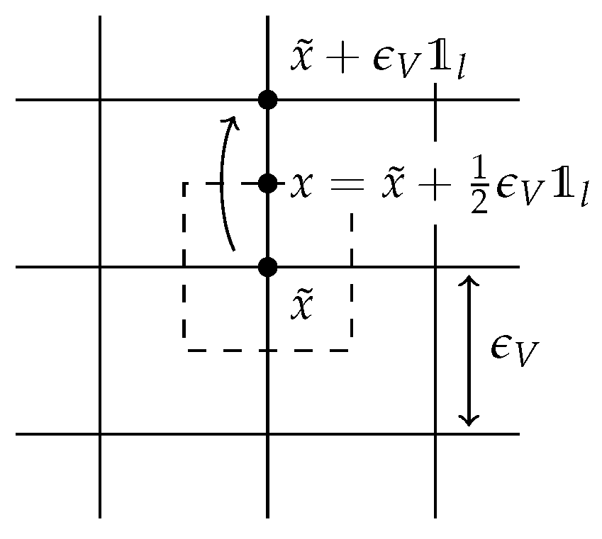
Now
measures the number of particles present in (lattice points in) an area
, while
measures the
net number of particles that have jumped through all midpoints in
, in direction
, for
, see
Figure 2. Note that both
and
are defined as measures on the lattice with shrinking distance
between lattice points; this measure-valued formulation is needed to pass to a continuum limit later on.
The concentrations and fluxes are related by the
V-dependent continuity equation:
Using that
, the integrated flux
is a Markov process in
with generator
Here, the factor comes from the time scaling , together with the fact that we have independent particles to choose from.
5.2. Limit and Large Deviations
For a test function
, we set:
The continuity Equation (
47) converges to the limit continuity equation (with the usual divergence operator):
With this notation, as
the generator (
48) converges to (if
):
As in
Section 2.3, the limit generator depends on derivatives of the test function only, and so the process
converges (pathwise in probability) to the deterministic path satisfying Fick’s Law:
Naturally, combining this equation with the continuity Equation (
49) yields the diffusion equation for the empirical measure:
Similarly, we derive the dynamic large deviations by studying the non-linear generator:
which follows from expanding the exponentials (with order-
exponents) up to second order. Then the following large-deviation principle on flux space holds:
with
Note that
is independent of
, and by (
51), the invariance condition (
28) is satisfied. Hence by the contraction principle (Theorem 4.2.1, [
23]), one obtains the large-deviation principle corresponding to the states (empirical measures):
with
using the notation
.
5.3. Induced GGSs in Flux and State Space
We can now apply Theorem 1 to extract a GGS from the L-function
. We first choose the ‘naive’ flat manifold of non-negative vector measures
(equipped with the flat total variation metric). It is easily checked that condition (34) holds for the free energy given by:
where we identify
, and we implicitly set
whenever the measure is not absolutely continuous. (This expression can again be seen as a relative entropy, cf. (
22), but now with respect to the Lebesgue measure, where the measure of the whole space—in this case infinity—is omitted. See also (Proposition 3.2, [
4]) for a general result in locally finite measure spaces). The dissipation potentials are obtained from (
36) and (
29), which yields
Theorem 1 states that induces the GGS on flux space.
For the state space, it is well-known that the state L-function (
52) induces the entropy-Wasserstein gradient flow of the entropy functional [
4,
26,
27,
28]. By the theory developed in
Section 4, we can now see how this gradient structure is related to the flux gradient structure. Indeed, the flux free energy
depends on state only, i.e.,
, where
, and so by Proposition 2 the state L-function
induces a GGS driven by
. Moreover, since the invariance condition (
28) holds, the dissipation potentials are related by Equations (
44) (recall the norms introduced above in (
52)):
5.4. A New Geometry
The form of the dissipation potential
and
suggests that it is more natural to use different manifolds in the spirit of Remark 2. For the state space this points to the space
of probability measures of finite second moment space, equipped with the Monge–Kantorovich–Wasserstein metric [
29]:
with tangent and cotangent space
and
. For this setting, the inverse metric tensor
is known by the Benamou–Brenier formula (Theorem 8.1, [
29]) to be
, so that the GGS is indeed the entropy-Wasserstein gradient flow [
30]:
Motivated by this observation we can take for the flux manifold the space of signed vector measures of finite
first moment
. This choice guarantees that the corresponding states have finite second moment (once
):
Moreover, we can now use the dissipation potential to construct a natural metric on
:
where the infimum runs over paths of fluxes for which
remains non-negative. The corresponding tangent and cotangent spaces (in the interior of the domain) are simply
and
and the inverse metric tensor
is
. This yields an interesting geometry in flux space, which, as far as the author is aware, is still unknown in the literature.
6. A Simple Reaction-Diffusion Model
We now combine the models from
Section 3 and
Section 5 to study reaction-diffusion models in flux and state space. The stochastic particle system will now consist of ‘reacting random walkers’. It is known that, if the reaction networks include reactions of different orders (unimolecular, bimolecular, etc.) and we only allow particles to react if the required number of particles are present within the same site/compartment, then the model may not converge to the expected reaction-diffusion Equation [
31]. The reason behind this is that for a multimolecular reaction, it becomes very unlikely that the required amount of reactants are all within one site/compartment; different order reactions would require different scalings. This is beyond the scope of the current paper. However we can already illustrate the combination of reaction and transport fluxes for a simple system of unimolecular equations of the type:
In this section we consider GGSs only, hence we shall always consider net rather than one-way fluxes.
6.1. Reacting and Diffusing Particle System
Since we consider unimolecular reactions only, we can take
independent reacting random walkers on the scaled lattice
, where each reaction occurs locally at each lattice site with rate
or
respectively, so that
For the transport mechanism, we assume that the two species hop to neighbouring lattice sites with rates and respectively.
As before we consider the random concentrations, as well as the integrated (net) fluxes, where we now distinguish between
transport fluxes and
reaction fluxes. If
is the position and
is the species of the
i-th particle, then
The concentrations and fluxes are again related by a continuity equation:
where the discrete divergence is as in (
47), and
is the matrix consisting of one state change vector corresponding to a forward reaction.
The pair
is then a Markov process with generator
where
6.2. Limit and Large Deviations
By the same procedure as in
Section 2.3 and
Section 5.2, one finds that as
and
, the continuity operator (
56) converges to (assuming
):
and the process converges (pathwise in probability) to the solution of the system:
Indeed, putting these together yields the reaction-diffusion equation for the limit concentrations:
To find the corresponding large deviations, we combine (
17) and (
50) to calculate the non-linear generator:
Let us again abbreviate
and
. The limiting non-linear generator can now be split into
Since each mechanism corresponds to a separate flux, the corresponding L-function also splits into two parts:
using the usual the relative entropy between two measures, i.e.,:
if
, else
.
As before, the calculation above formally shows that the flux large-deviation principle holds (see for example [
32] for a similar but rigorous result):
The L-function (
59) splits into two parts because the only interaction between the two mechanisms occurs through the state
. By contrast, the corresponding state space large-deviation are much more complicated. Observe that the continuity Equation (
57) is an affine function of
, and so
is independent of
, and the invariance condition (
28) holds. As explained in the beginning of
Section 4, this means that one can apply a straightforward contraction principle on the tangents to yield the large deviation cost function for the states/concentrations:
This infimum reintroduces a strong interrelation between the two driving mechanisms. Indeed, for a given tangent
, the fluxes in this infimum correspond to an optimal splitting between the two mechanisms, which can be seen as an inf-convolution. Similar interactions also arise when considering multiple reaction pairs, see (Section 3.4, [
16]).
6.3. GGSs in Flux and State Space
We now apply Theorem 1 to the reaction-diffusion setting. The symmetry condition (34) holds for the function (
58) if we choose the free energy functional
Naturally, this functional can be seen as a combination of (
22) and (
53), where just like (
53), it has the form of a relative entropy with respect to a locally finite invariant measure, namely
. We find the corresponding dissipation potentials from (
43), which is again a combination of the non-quadratic potentials (
23), (
24) and the quadratic potential (
54):
with
. Let the flux space be given by
, where the first two spaces, corresponding to the transport fluxes, are equipped with the metric (
55) introduced in the previous section. By Theorem 1 the flux cost function
induces the GGS
. We stress that the dissipation potential
splits into two potentials for the transport and reaction mechanisms respectively, but the free energy is one and the same for both mechanisms.
Since a GGS is a special case of a pGGEN, by Theorem 3, the state cost function
also induces a GGS
, in this case in the space
. The same result yields
and, using
:
We stress that, analogous to the L-function (
60), the dissipation potential
on state space no longer splits into two parts.


