Abstract
During the assembly process, there are inevitable variations and noise factors in the material properties, process parameters and screening scheme, which may affect the quality of the product. Using the stress-strength model, an evaluated screening scheme method, by analyzing the variation of the defect density in the assembly process, is proposed and discussed. The influence of screening stress on product defects is considered to determine the screening scheme. We performed the defect stream analysis by calculating the recursive relations of residual defect density under multi-stress conditions. We find that the probability density function, which shows the defect changing process from latent to dominant relative to the time process, agrees very well with the historical data. We also calculate the risk as the entropy of the assembly task. Finally, we verify our method by analyzing the assembly process of a certain product.
1. Introduction
In the lifecycle of mechanical product manufacturing, the quality of the product depends on the quality of the assembly process [1]. A fatal or killer defect is one that is of sufficient size and occurs in a place where the outcome is an immediate device failure [2], for example, when the product size exceeds the design threshold after processing; such a defect is detected after the manufacturing or screening test. A defect that is either too small or is located in a position that does not cause an immediate failure is called a latent defect. A latent defect may or may not cause failure in the field, depending on the operation time, environmental condition and processes [3].
In the evolution of the potential defects, potential defect analysis is performed to determine the dominant influence on the reliability of the product, which can help to determine the most reliable assembly sequence and screening position. Previously, there were some attempts to extend defect models to estimate reliability. A simple time-independent Poisson reliability was obtained by directly assuming that the number of nonfatal defects is proportional to the number of fatal defects following a Poisson distribution [4,5,6]. But only cases of the distribution of defects following a certain law are analyzed and they were not completely applied to the assembly process. In addition, all these models implicitly assumed that the number of fatal defects is independent of the number of the latent defects in a device.
Different resistance strengths of products corresponding to different stresses in the assembly process will result in different defects if the strength threshold is exceeded. Whitney et al. [7,8] presented a residual strength degradation model which deals with both tensile and compressive strength degradation as competing failure modes. Xie et al. [9] established a direct correlation between the failure rate and failure-controlling variables and analyzed the causal relationship between the failure rate curve shape and the probabilistic property of the load-strength interaction, developing a load-strength interference relationship-based failure rate model. Despite the extensive studies on competing failure models, we notice that few works have focused on the impact of stresses on different failure modes. This motivates us to investigate the impacts of different stresses from the perspective of the failure rate [10]. Such processes are often “competing”, leading to failure [11] and may be dependent on each other in a number of ways; in this case they are referred to as dependent competing faire processes [12]. Various dependencies have been discussed in the literature, e.g., the statistical dependency described by joint probability distributions [13,14], copulas [15,16], and the functional dependency described by failure propagation and isolation [17,18,19,20,21]. In this paper, we consider the dependency between two types of failure. Different screening methods aim at different product defects, so the first innovation of this paper is to establish the relationship between stress and defect by quantifying the stress of the assembly process, so as to optimize the selection parameters more precisely. Models consider both degradation and the relationship between stress and strength during the assembly process.
Environmental stress screening (ESS) refers to the process of exposing a newly manufactured or repaired product or component (typically electronic) to stresses such as thermal cycling and vibration in order to force latent defects to manifest themselves by permanent or catastrophic failure during the screening process. Although there have been some empirical studies on the ESS in the literature, the study conducted by Cha and Finkelstein et al. [22,23,24] is the first to deal with adequate stochastic modeling, analysis and optimization of the ESS. Elskamp and Peng et al. [25,26] analyzed the effect of the screening; Kumar and Omar [27] quantized the screening procedure; Khatibi and Suhir et al. [28,29,30] studied the electronic parts with the ESS. However, the screening process was not quantitatively analyzed from the perspective of defect. The second innovation of this paper is to optimize the screening parameters in the selection scheme by quantifying the defect density of the product in the assembly process.
The paper is organized as follows. In the next section, we use the stress-strength model to analyze defect generation in the assembly unit. Then, an assembly process model is developed to describe the defect stream during this process, which considers the defect changing process from latent to dominant relative to the time process. The failure efficiency of the product under different stress levels is calculated by considering the multi-stress strength interference model under the result of competitive failure. Then, the risk of the improved screening method is evaluated by calculating the change in the defect density. Finally, an example related to a printed circuit board assembly (PCBA) is analyzed by our model.
2. Stress-Strength Model in Assembly Unit
2.1. Defect Analysis in Assembly Unit
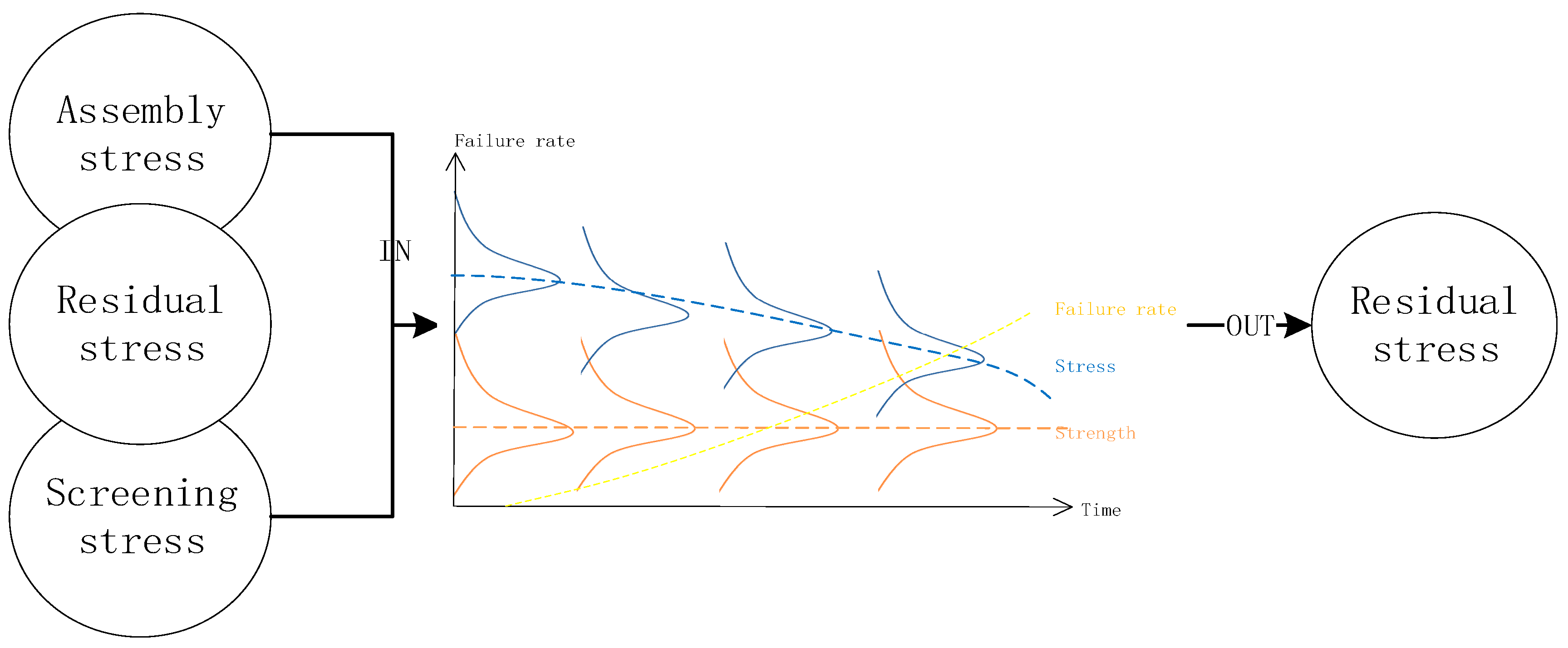
The quality of assembly is the result of the interaction of multiple processes. Each process has the effect of optimizing the quality of the product and increasing the potential defects of the product. There is also the stimulation and correction of the potential defects of the product between the processes. In other words, each process is the correction and inheritance of the potential defects left over from the previous processes. Therefore, this section analyses the defect generation and rejection of the single process in the assembly.
As shown in Figure 1, potential defects may be introduced in the assembly process or the potential defects may be fired as a dominant defect during the assembly task. The model developed in this paper is motivated by the actual engineering problem of modeling the analysis of printed circuit board (PCB) assembly. A PCB is subject to two main failure mechanisms: one concerns the electro- migration, the other one involves the component solderability. This paper assumes that the assembly phase of each process is subject to the same distribution D and the defect is limited for each process to a single stress action. Therefore, the stress strength interference model based on the competitive failure algorithm is established to analyze the resistance strength of PCB under different stresses, and the product failure efficiency under corresponding stress is obtained.
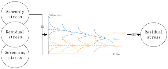
Figure 1.
Defect analysis in assembly unit.
2.2. Stress-Strength Model with Competing Failure
For structural reliability, the failure of a system occurs when the stress modeled by an external shock process exceeds the strength of the system for the first time. In practice, the probability of this failure depends on the magnitudes of the previously survived shocks. The stress-strength interference model and reliability calculation formula are the basis of reliability design and failure analysis [31], but in many cases they are difficult to direct. The main reason for the application of engineering calculation is:
- Lack of distribution data;
- There are several random variables affecting product reliability, and the stress-strength interference model cannot be applied directly to n-dimensional vectors.
In this paper, according to the known requirements of product reliability and the stress distribution in the assembly process, because the assembly process is too complicated to express the strength completely with a distribution, the product strength requirement that satisfies the product reliability requirement under the stress of the assembly process is obtained by a linear search method. The product strength obtained is taken as the standard to measure whether the assembly process can meet the product quality. The residual defects affect the strength of the product, so the relationship between the potential defects, the stress in the assembly process, and the reliability of the product is established.
We have defined the auxiliary function , where xi (i = 1, 2, ..., n) represents various random stresses during the assembly process and xn+i is the strength under xi stress. This function is called a multivariate function, representing the state of the product. When Z > 0, the intensity is greater than the stress; when Z < 0, the strength is lower than the stress. Let xi follow a normal distribution with an average μi and a standard deviation σi; according to the linear search method, the main steps are as follows:
- Step 1: Assign the initial value to each random variable, generally taking the average value of each variable;
- Step 2: Compute the partial differentiation of function Z at the current value point of each random variable ;
- Step 3: Compute the sensitivity coefficient :
- Step 4: Compute the reliability coefficient β:
- Step 5: Insert β into the formula below and obtain the new value of xi*:
Repeat step (2) to step (5) until the difference between the resulting β and the previous β is less than the tolerance error. At this point the obtained x* = (x1*, x2*, …, x2n*) is the design point to meet the reliability requirements. xn+i* represents the optimum strength value to meet the design requirements and reliability requirements; there is a corresponding xi* under each process, establishing a strength interval based on the strength value required by the product.
Stress levels are selected, of which S0 is the normal stress level, Si (i = 1, 2, …, n) is the higher stress level of a kind of stress which is calculated from the stress-strength model. For example, in the case of this paper, three stresses levels were selected: S0 is the normal level, S1 is the higher stress level of mechanical stress, and S2 is the higher stress of thermal stress. The product reliability requirement and design requirement could be met under these kinds of stress:
- Product failure is caused by only one of the two failure mechanisms, T1 and T2 represent the occurrence time of mechanism 1 and mechanism 2, respectively; they are independent of each other, and the product life is T = min(T1, T2)
- At the normal stress level, the occurrence time of mechanism j (j = 1, 2) obeys the Pareto distribution, and its reliability function and inefficiency function are, respectively:where is the scale parameter, is the shape parameter and they are known.
- At stress level Si, the failure rate function of mechanism j (j = 1, 2) is:
The corresponding reliability value is brought into the calculation of acceleration factor .
3. Screening Scheme Evaluation with Defect Stream Analysis
3.1. Defect Stream Modeling
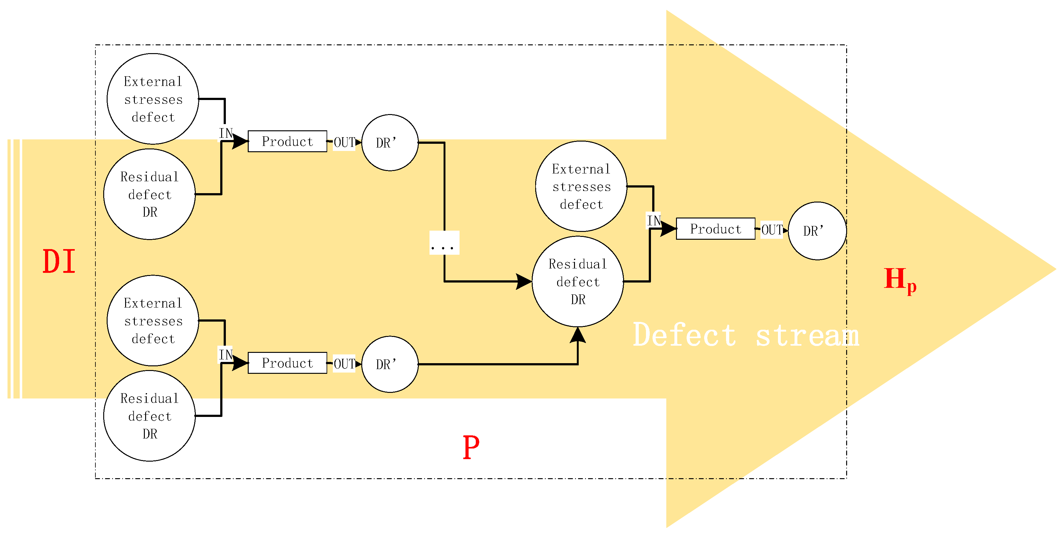
Different assembly units have different effects on product defects. Set an assembly task as a three-dimensional vector A (DI, P, Hp), where DI is the initial value of defect density, P is the set of processes included in the assembly task, Hp is the value of risk evaluation for this task (Figure 2). The risk of the process can be reduced by the modification of each procedure in the deployment task. Assembly process defect analysis based on defect flow is shown in Figure 2.
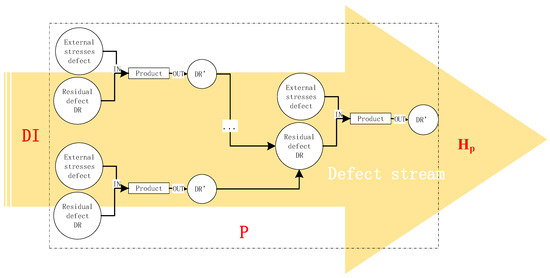
Figure 2.
Defect stream of the assembly process.
This paper also considers the influence of screening stress on product defects to determine the screening scheme. Theoretical analysis shows that after environmental stress screening (ESS), the product will improve the early failure rate. The evaluation of the screening procedure is shown:
where λ0 is the specified failure rate determined by the actual target of reliability, λD is the early failure rate, D is the residual defect density after the ESS, and T is the early failure time. R0(t) is the product reliability before screening, Ra(t) is the reliability after screening. The change of the evaluation value of the product before and after screening is:
3.2. Quantification Defines Defect
Various types of defects are introduced in the design and manufacturing process, which are mainly divided into three categories: design defects, technological defects and components defects. However, the design defect cannot be screened by the environmental screen stress. In the actual assembly process, defects are derived from process stress, screening stress and potential defects after the previous procedure. Because the ESS does not screen design defects, if the stress screening is carried out in the previous step, the design defect needs to be subtracted from the current node. This paper assumes that the design defect is a constant value during the assembly process:
where and represent the respective screen defects density and the number of defects density remaining in the previous step. Therefore, the screening degree can be improved indirectly through the analysis of the relationship between various defects of different location nodes.
In Figure 3, the black rectangle represents the process node and the middle (green) square represents the state after screening. If there is no screening, the defect density in the middle (green) square is equal to the density in the black rectangle; in other words, if no new processes are added, the defect density of the product remains unchanged. Conversely, the red one represents the screening node, i.e., the introduced screening stress; the input of the defect would be added. Before the environmental screening stress test, y% is the percentage of the defect density of the components. After screening, the ratio of the theoretical value to the actual value of the screening test is x%. We establish the relationship between x and , where , and TS represents the degree of screening or indicates the extent to which the process corrects such defects. M is the total number of defects after each screening (this article assumes that there are only two types of defects in the assembly process, M1 is the first type of defect, M2 is the second type of defect, M1 + M2 = M). Based on the historical data, the probability density function D that shows defect changing process from latent to dominant relative to the time process, was fitted.

Figure 3.
The model of defect density
It is assumed that the design defect will not be transferred to other defects throughout the process, so x after screening is:
where is the parameter according to the specific assembly process. Because of the structure of assembly chain, the method of defect density calculation changes within different location of the nodes. The following two cases are discussed: one case considers the leftmost endpoint node in Figure 2; the other case considers the intermediate nodes. The endpoint node indicates that the product is not elaborated on before this process; for each node, the total number of latent defect depends on the previous procedures. The serial structure and parallel structure would be different for calculating . First, the problem is simplified, and the number of left connected nodes in each process is considered to be 1 (Dij indicates class i defect found in operation j).
Latent defects and dominant defects exist in the probabilistic assembly process, in which the potential defects are transformed into dominant defects. If the latter is activated, then the product fails, and the next assembly stops. Considering the definition, the potential defects and dominant defects in the assembly process are subject to exponential distribution. The time hypoexponential distribution of the whole assembly process defect change is expressed below.
In the distribution, two parameters are present (). The same mean and sample coefficient of variation (c) are collected from the history data. The variation coefficient c is always < 1. The parameters and can be estimated as follows:
The resulting parameters and are real values if . This paper assumes that the total defect is D; each time there is a probability of the first type of defects (component solderability), there is a probability of the second type of defects (electro migration), where + = 1.
3.3. Quantitative Characterization of Defect Stream
1. The start node
There is no latent defect introduced from previous operations in the node at the start point:
We simplify this by using power series. represents the unreliability of the product, N is the number of circle nodes representing the screenings, TS is the degree of the screening, and λD depends on the stress of the screening. In this paper, λD is calculated by the competing failure model based on the stress-strength. The relationship between the degree of ESS and the latent defect (DR = DIN (1 − TS)) is:
2. The intermediate node
For intermediate nodes representing remaining potential defects after a process, the previous phase is completed in parallel by multiple operations. The reliability of the defects would be greatly reduced because the stress screening needs to eliminate as much as possible the remaining potential defects, reducing the risk of assembly. The failure rate λD is calculated by the competing failure model. DS1 represents defects introduced by vibration screening; DS2 represents defects introduced by temperature cycle screening.
It can be concluded that each node is related to the previous node, and the recurrence relationship is as follows:
Only one type of screening is performed at a time when the type of screening is temperature screening (the same applies to the calculation of defect flow in vibration screening):
The residual defect density of each node is obtained according to the recursive formula. To generalize the problem, the left connected node is not 1. This means that there is no parallel assembly of multiple operations before a single operation. In other words, there are more processes that affect the defect density of the product. The calculation of parallel nodes mainly considers the residual defect density in the combined node, as shown below: in this paper, m is the number of the left nodes:
The parallel system is assembled from multiple parts to components, so the stress levels in each part are different, and the values of each residual defect density are different. The residual defect density after screening is as follows: only one type of screening is performed at a time, when the type of screening is temperature screening (the same applies to the calculation of defect flow in vibration screening):
For series and parallel nodes, the residual defect density of the current node can be represented by a recursive equation. The other parameters can be analyzed by the specific assembly process.
3.4. Screening Scheme Evaluation
The total number of defects in the product after the assembly process is the input I; the defective products are detected by the buffer after the process; they return to the buffer before the process if this process needs to be screened. The residual potential defects in the final output of the assembly process after n tests are O; no screening, O = I. When the input is greater than the output, the assembly process risk is low and can meet the requirements of the assembly; when the input is less than the output, the high risk of the assembly process cannot meet the requirements. The purpose of the study of assembly process risk is to reduce the assembly process risk and improve the assembly quality by optimizing the assembly process and increasing the screenings.
The process risk of the assembly process is evaluated by the entropy. Entropy represents the degree of confusion within the system. Accordingly, if the entropy is close to 1, the system is more chaotic, and the control ability of the system is poor. The calculation of entropy not only characterizes the risk of assembly process but also characterizes the complexity of the assembly process, which can help us make better decisions. This means the entropy of each process Hpi and the entropy of the assembly process H are calculated in this way:
where k = [0, n], k ∈ N, n is the total nodes of the assembly process. Based on the residual defect analysis, the evaluation of the screening procedure is calculated as the change of the residual defect density:
where t is the total time required to complete the current process. Combined with the previous analysis, we obtain:
We find the best screening method of the assembly process by means of recursive optimization. The derivation process of the recursive relation will be explained in detail later.
4. Case Study
At present, PCBAs play an increasingly important role in various fields and have become more popular and customized. In the manufacturing process of PCBAs, the workload of the assembly process accounts for more than 50% of the total workload. The assembly process of the flight control of a PCBA is analyzed as an example. As a fragile part in the assembly process, PCB is analyzed in this case mainly for the defects of the PCB board in the assembly process. Using work breakdown structure (WBS) to find the key components, the flow chart of these key components in the assembly process is shown in Figure 4.
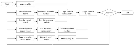
Figure 4.
The flow chart of the assembly process of a flight control module.
Steps 1–4 describe the process of using the method in this paper for this case:
Step 1: Determine the process flow and the number of the process
The main processes of the assembly process are: mechanical clamping, surface mount technology (SMT) and wave soldering. All the processes are shown in Figure 5.

Figure 5.
The flow-chart of the process.
Step 2: Fitting the function of stresses
Monitor the previous process by the sensor and collect the stress data of the assembly process to fit the stress distribution. Select the key position on the assembled workpiece.
The optimized function F(x) of loading stress with 95% confidence bounds is:
The optimized function F(x) of the SMT process with 95% confidence bounds is:
The optimized function F(x) of the waving welding process with 95% confidence bounds is:
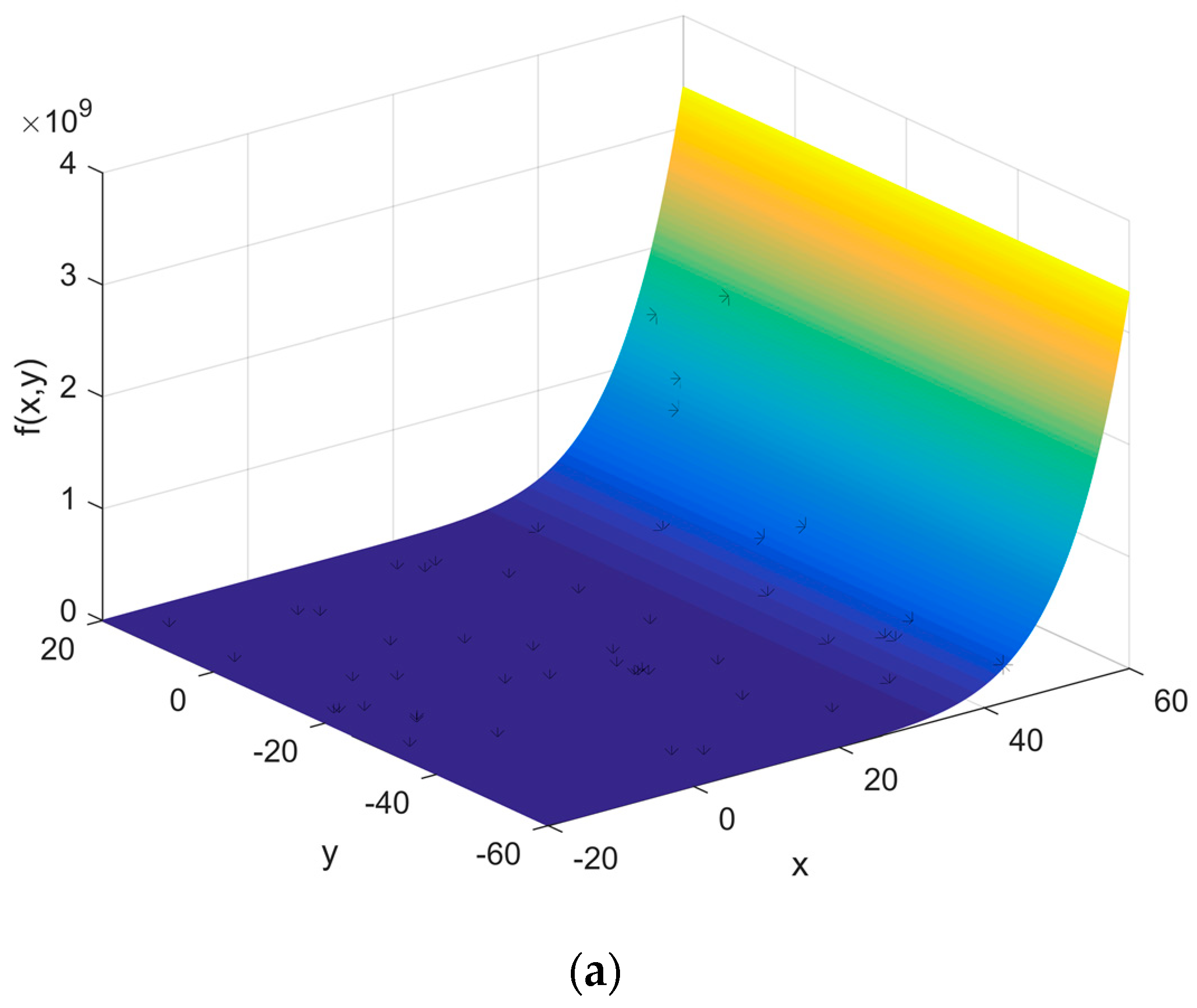
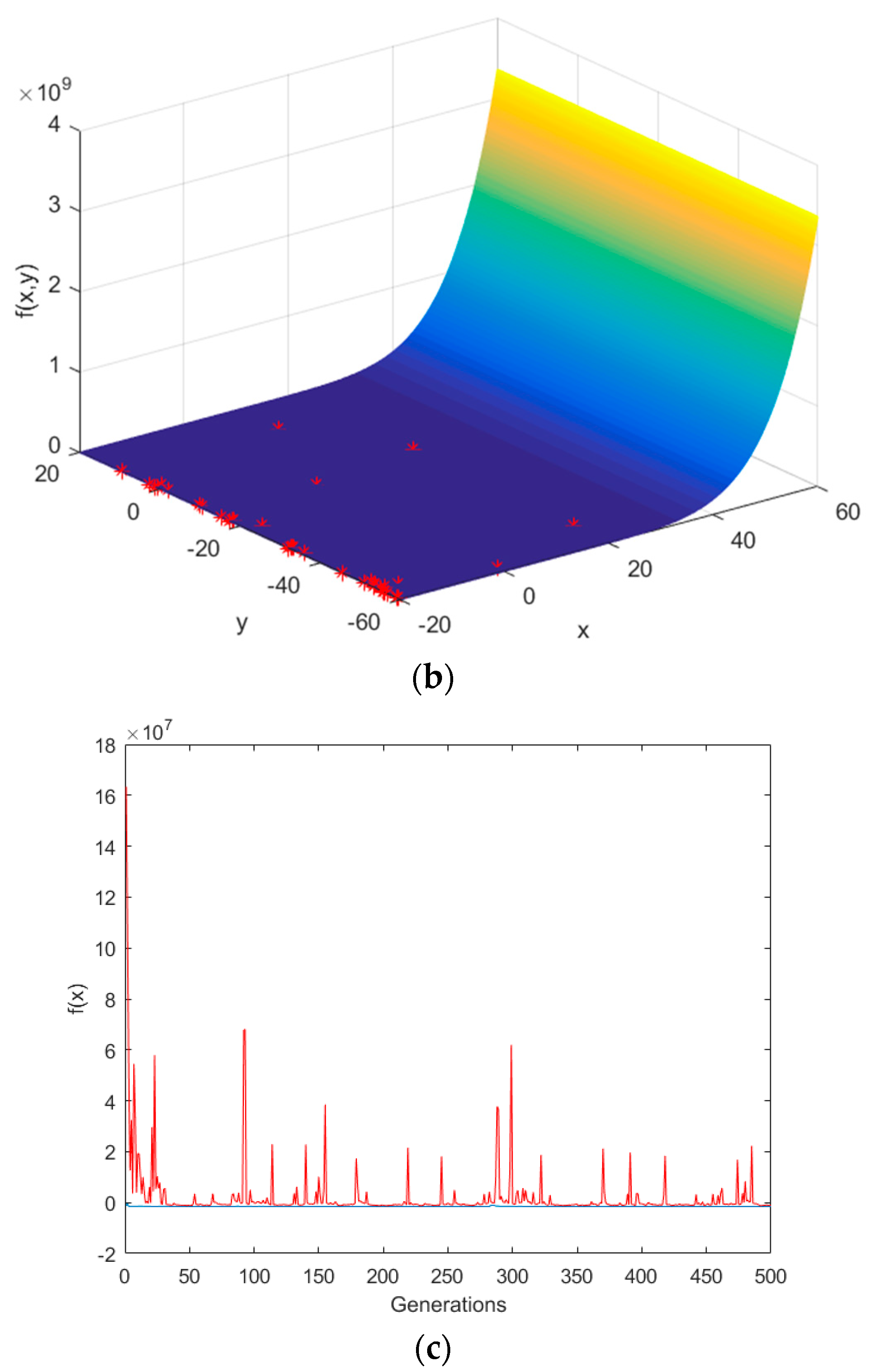
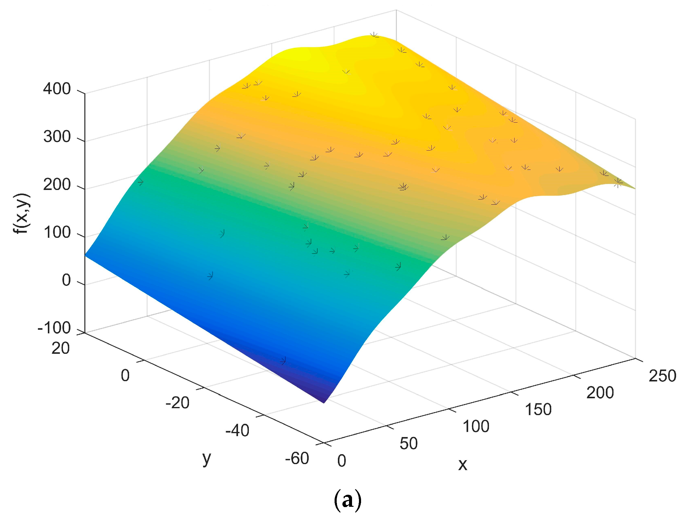
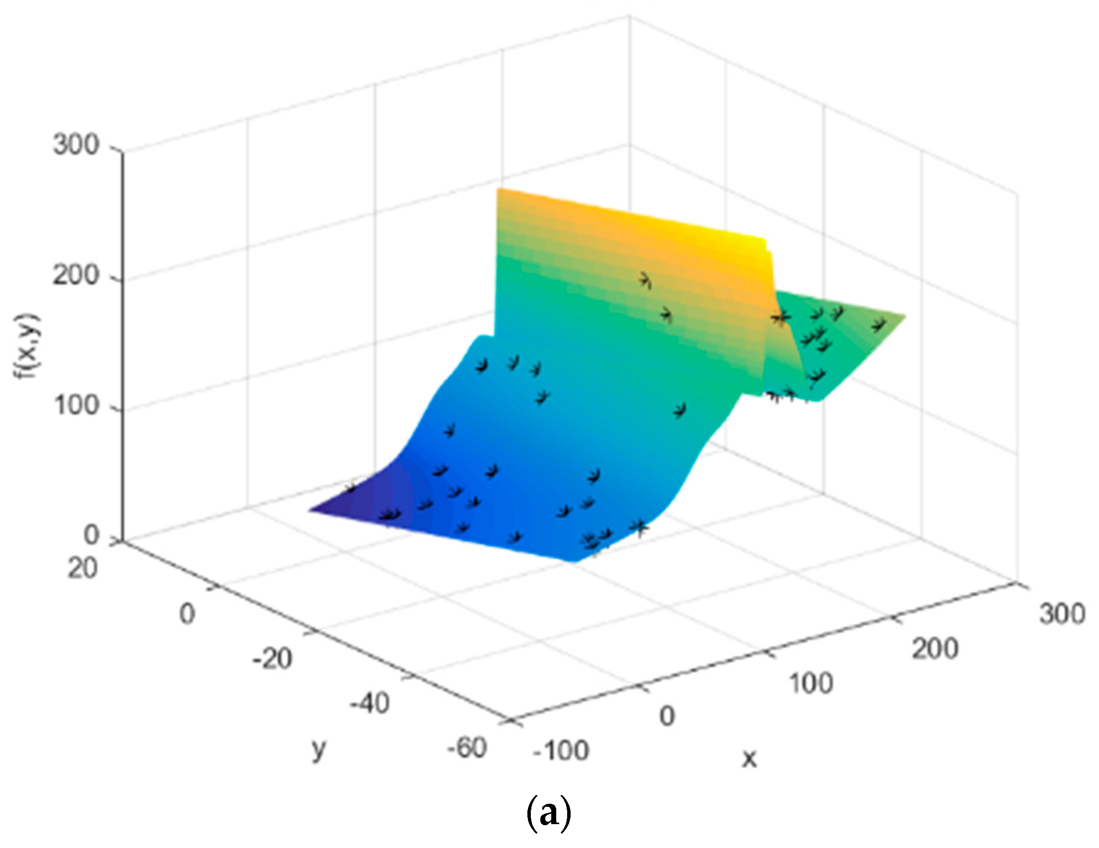
The stress distribution is brought into the multivariate function Z and the minimum value of Z in the range of stress and strength is obtained by genetic algorithm. At this point, the optimal stress value for the maximum strength under the guaranteed reliability level of the process is calculated. The calculation process is shown in Figure 6, Figure 7 and Figure 8 and the results are shown in Table 1.


Figure 6.
Maximum loading stress found. (a) The initial position of the chromosome; (b) The final position of the chromosome; (c) The optimization process.
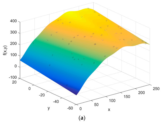
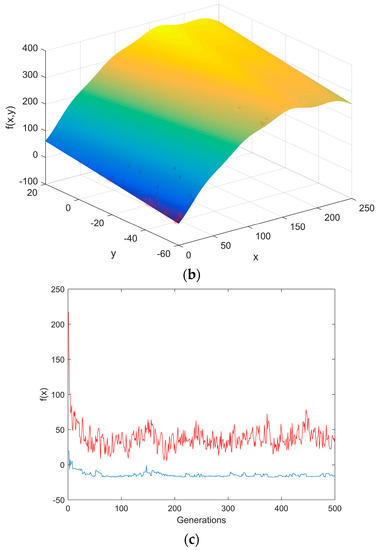
Figure 7.
Maximum SMT found. (a) The initial position of the chromosome; (b) The final position of the chromosome; (c) The optimization process.

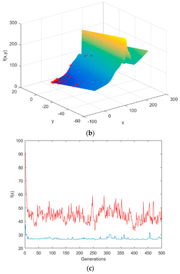
Figure 8.
Maximum waving welding found. (a) The initial position of the chromosome; (b) The final position of the chromosome; (c) The optimization process.

Table 1.
The result of the stress-strength model.
Step 3: As far as the above three stresses are concerned, the effect of the mechanical assembly process on product quality should be paid more attention in the assembly process.
Three stress levels are selected, of which S0 is normal stress level, S1 and S2 are the high levels of loading stress and hot stress, respectively; the product reliability requirement and design requirement could be met under three kinds of stress:
1: Product failure is caused by only one of the two failure mechanisms; T1 and T2 represent the occurrence time of mechanism 1 and mechanism 2, respectively, and they are independent of each other; the product life is T = min(T1, T2).
2: At the normal stress level, the occurrence time of mechanism j (j = 1, 2) obeys the Pareto distribution, and its reliability function and inefficiency function are, respectively:
where is the scale parameter, is the shape parameter and they are known.
3: At stress level S1, the failure rate function of mechanism j (j = 1, 2) is:
The corresponding reliability value is brought into the calculation of acceleration factor . ; the result of the parameter fitting is shown in Table 2.

Table 2.
Parameter fitting result.
Obtain the acceleration factor to calculate the failure rate:
Step 4: Screening optimization
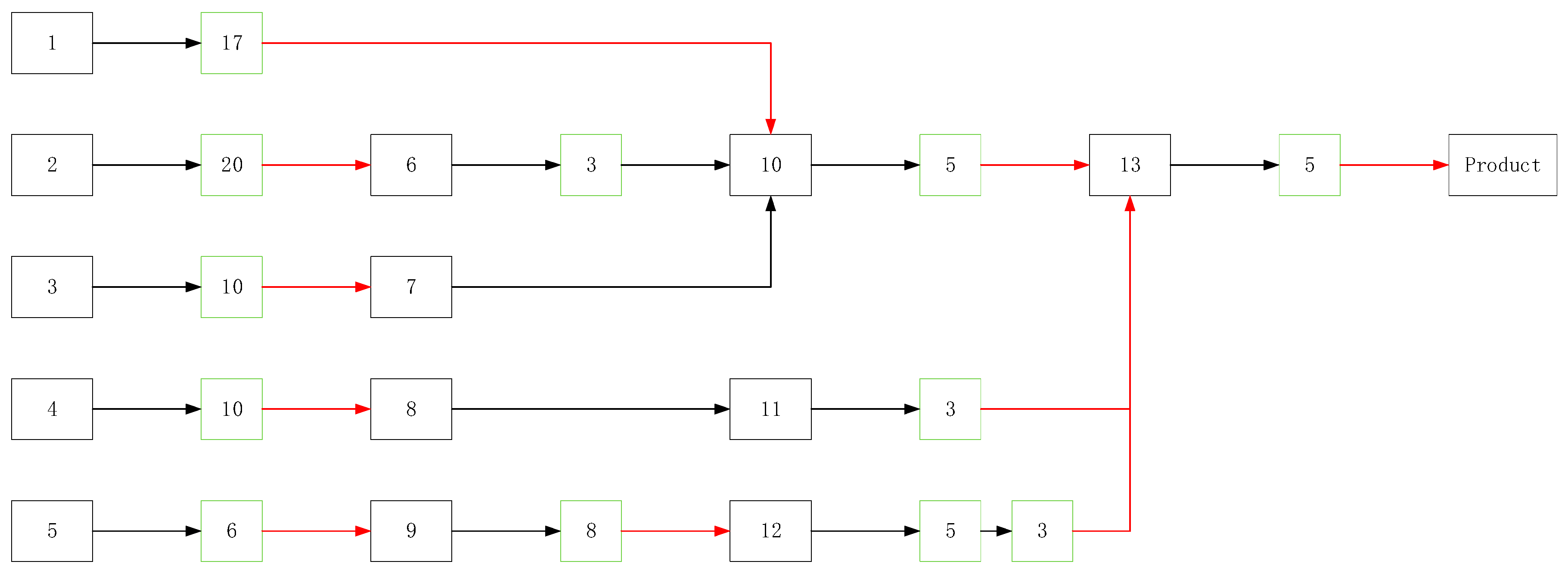
The assembly chain is numbered, and the relevant parameters are calculated according to the original assembly sequence and selection scheme. Figure 9 is an existing assembly scheme. We analyze and optimize this process.
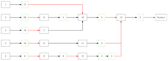
Figure 9.
Historical screening program.
In Figure 9 the green square is the node of screening, and the number in the green square represents the temperature cycles (where, for this case, the range of the temperature cycle is −50 °C–70 °C (R = 120), the rate of the temperature change v is 10), and the red connector indicates 20 min of random vibration filtering. For this screening program, after the process of No. 7 and No. 8 without screening, No. 9 conducted a second screening. The number of problems in the actual production process, the screening strength and the screening position of each screening point of the original screening scheme, and the failure rate of the assembly process, are obtained through the historical production data. Combined with the recursive function of residual defect density DR deduced in this paper, we calculate the residual defect density in every node of this assembly process by the original screening scheme. The other parameters are calculated before with the historical assembly process data. No. 10 and No. 11 are parallel nodes, and the remaining nodes are series nodes.
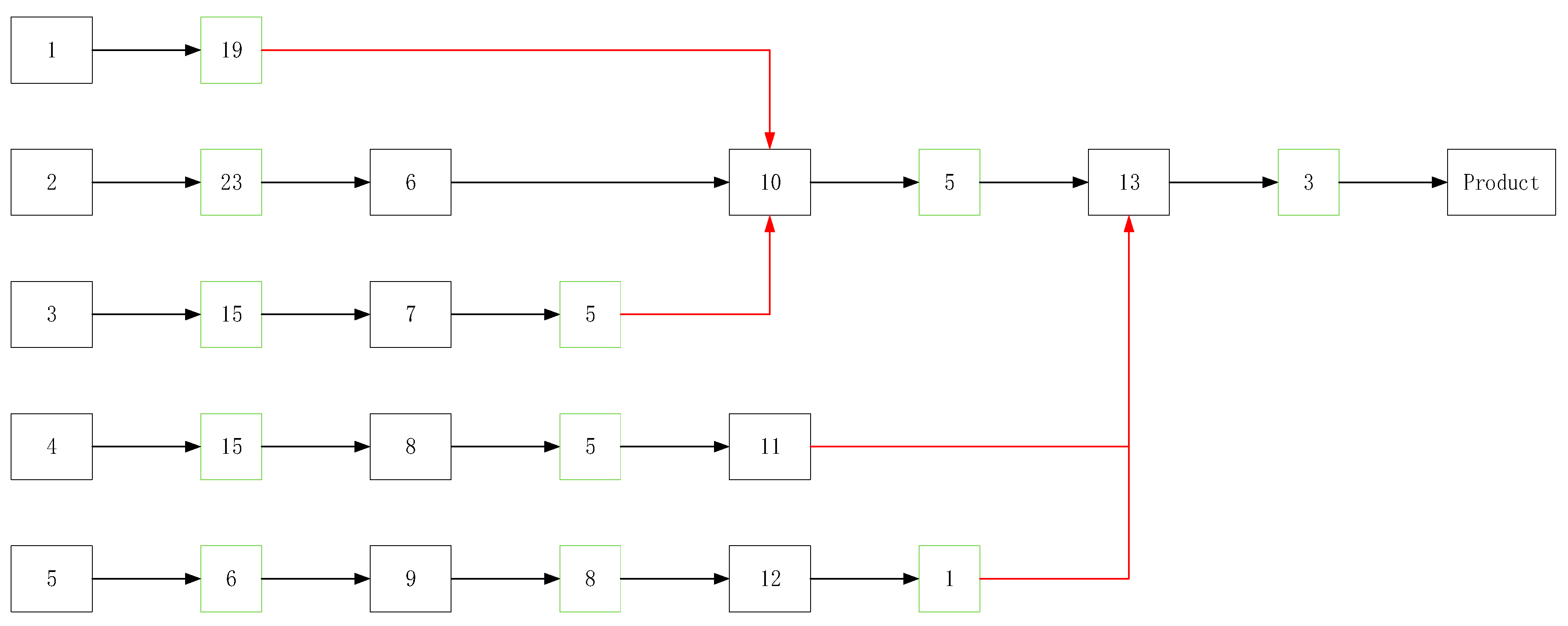
As shown in Table 3, the first point, after the secondary screening of the node No. 12, is that the defect of the screening stress increases the intrinsic residual defect density in the product. The entropy of the low-levels, the nodes in which I = 1, is less than in the other parts. However, under the good screening scheme, the number of problems should decrease with the increase of j. So, we need to strengthen the low-level screening. Based on the recursive relationship of defect density, the optimal selection scheme is found and is shown in Figure 10.

Table 3.
The entropy of the assembly process.
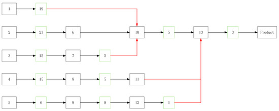
Figure 10.
Screening optimization.
Based on this program, the entropy of each node is in Table 4.

Table 4.
The entropy of the new screening.
5. Summary and Conclusions
In this study, the multistage assembly process is analyzed, and the effect of defect changes on product quality during the assembly process is also investigated. Through the analysis of the assembly task, the recursive relationships of residual defect density under multi-stress are obtained, and the defect analysis is quantified. The results of the probability density function that shows the defect changing process from latent to dominant upon the time process agree with the historical data. The definition of entropy in physics was used to characterize the risk of the model that evaluates the assembly process and the screening effects. Finally, we analyze a case for a flight control module assembly process in a PCBA to illustrate the effectiveness of our approach. Our result shows that the screening program can be improved.
In this paper, the effect of multiple stresses on different kinds of defects is not fully characterized quantitatively. Therefore, we will focus on the coupling effect of multi-stress on product quality for more precise selection of defects produced in the assembly process in our future work.
Author Contributions
W.D. and L.L. conceived and designed the experiments; Y.Z. analyzed the data. Y.H. performed the experiments and built the model. W.D. and Y.H. contributed to the writing and editing of the manuscript.
Funding
This work was supported by the Technical foundation program (Z132014A002) from the Ministry of Industry and Information Technology of China.
Conflicts of Interest
The authors declare no conflict of interest.
References
- Zhang, J.; Li, Y.; Yu, J.F.; Zhang, K.F. Producing performance analysis method for aircraft assembly unit based on Markov chain. Comput. Integr. Manuf. 2010, 16, 1844–1851. [Google Scholar]
- Kim, K.O.; Zuo, M.J.; Kuo, W. On the relationship of semiconductor yield and reliability. IEEE Trans. Semicond. Manuf. 2005, 18, 422–429. [Google Scholar] [CrossRef]
- Huang, Y.; Dai, W.; Mou, W.; Zhao, Y. Uncertainty evaluation in multistage assembly process based on enhanced OOPN. Entropy 2018, 20, 164. [Google Scholar] [CrossRef]
- Franciosa, P.; Palit, A.; Vitolo, F.; Ceglarek, D. Rapid response diagnosis of multi-stage assembly process with compliant non-ideal parts using self-evolving measurement system. Proc. CIRP 2017, 60, 38–43. [Google Scholar] [CrossRef]
- Siddiqui, J.; Ortega, J.; Albus, B. On the Relationship between Semiconductor Manufacturing Volume, Yield, and Reliability. In Proceedings of the IEEE International Reliability Physics Symposium Conference on Reliability Physics Symposium, Monterey, CA, USA, 2–6 April 2017. [Google Scholar]
- Kim, K.O.; Oh, H.S. Reliability functions estimated from commonly used yield models. Microelectron. Reliab. 2008, 48, 481–489. [Google Scholar] [CrossRef]
- Zhao, J.; Sun, Y.; Chai, L.; Li, P.; Lu, Y. Parameter analysis of defect rate of electrical equipment based on weibull distribution. Hebei Electr. Power 2015, 34, 1. (In Chinese) [Google Scholar]
- Whitney, J.M. A residual strength degradation model for competing failure modes. In Long-Term Behavior of Composites, ASTM STP 813; O’Brien, T.K., Ed.; American Society for Testing and Materials: Philadelphia, PA, USA, 1983; pp. 225–245. [Google Scholar]
- Xie, L.; Gong, Y. Series system failure rate modeling by load-strength interference analys. In Proceedings of the 2013 International Conference on Quality, Reliability, Risk, Maintenance, and Safety Engineering, Chengdu, China, 15–18 July 2013; pp. 78–80. [Google Scholar]
- Jiang, L.; Feng, Q.; Coit, D.W. Modeling zoned shock effects on stochastic degradation in dependent failure processes. IIE Trans. 2015, 47, 460–470. [Google Scholar] [CrossRef]
- Zeng, Z.; Kang, R.; Chen, Y. Using PoF models to predict system reliability considering failure collaboration. Chin. J. Aeronaut. 2016, 29, 1294–1301. [Google Scholar] [CrossRef]
- Huang, W.; Askin, R.G. Reliability analysis of electronic devices with multiple competing failure modes involving performance aging degradation. Qual. Reliab. Eng. Int. 2003, 19, 241–254. [Google Scholar] [CrossRef]
- Peng, H.; Feng, Q.; Coit, D.W. Reliability and maintenance modeling for systems subject to multiple dependent competing failure processes. IIE Trans. 2010, 43, 12–22. [Google Scholar] [CrossRef]
- Lai, C.D.; Xie, M. Stochastic Ageing and Dependence for Reliability; Springer: New York, NY, USA, 2006. [Google Scholar]
- Navarro, J.; Rychlik, T. Comparisons and bounds for expected lifetimes of reliability systems. Eur. J. Oper. Res. 2010, 207, 309–317. [Google Scholar] [CrossRef]
- Wang, Y.; Pham, H. Modeling the dependent competing risks with multiple degradation processes and random shock using time-varying copulas. IEEE Trans. Reliab. 2012, 61, 13–22. [Google Scholar] [CrossRef]
- Bunea, C.; Bedford, T. The effect of model uncertainty on maintenance optimization. IEEE Trans. Reliab. 2002, 51, 486–493. [Google Scholar] [CrossRef]
- Wang, C.; Xing, L.; Levitin, G. Competing failure analysis in phased-mission systems with functional dependence in one of phases. Reliab. Eng. Syst. Saf. 2012, 108, 90–99. [Google Scholar] [CrossRef]
- Wang, C.; Xing, L.; Levitin, G. Reliability analysis of multi-trigger binary systems subject to competing failures. Reliab. Eng. Syst. Saf. 2013, 111, 9–17. [Google Scholar] [CrossRef]
- Wang, Y.; Xing, L.; Wang, H.; Levitin, G. Combinatorial analysis of body sensor networks subject to probabilistic competing failures. Reliab. Eng. Syst. Saf. 2015, 142, 388–398. [Google Scholar] [CrossRef]
- Hao, S.; Yang, J. Reliability analysis for dependent competing failure processes with changing degradation rate and hard failure threshold levels. Compute. Ind. Eng. 2018, 118, 340–351. [Google Scholar] [CrossRef]
- Cha, J.H.; Finkelstein, M. On a terminating shock process with independent wear increments. J. Appl. Probab. 2009, 46, 353–362. [Google Scholar] [CrossRef]
- Cha, J.H.; Finkelstein, M. On new classes of extreme shock models and some generalizations. J. Appl. Probab. 2011, 48, 258–270. [Google Scholar] [CrossRef]
- Finkelstein, M.; Cha, J.H. Stochastic Modeling for Reliability; Springer: New York, NY, USA, 2013. [Google Scholar]
- Elskamp, F.; Kruggel-Emden, H. Review and benchmarking of process models for batch screening based on discrete element simulations. Adv. Powder Technol. 2015, 26, 679–697. [Google Scholar] [CrossRef]
- Peng, K.; Yilmaz, M.; Tehranipoor, M.; Chakrabarty, K. High-quality pattern selection for screening small-delay defects considering process variations and crosstalk. In Proceedings of the Conference on Design, Automation and Test in Europe, Dresden, Germany, 8–12 March 2010; pp. 1426–1431. [Google Scholar]
- Kumar, S.; Omar, M.K. Stochastic re-entrant line modeling for an environment stress testing in a semiconductor assembly industry. Appl. Math. Comput. 2006, 173, 603–615. [Google Scholar] [CrossRef]
- Moreno-Lizaranzu, M.J.; Cuesta, F. Improving electronic sensor reliability by robust outlier screening. Sensors 2013, 13, 13521–13542. [Google Scholar] [CrossRef] [PubMed]
- Khatibi, G.; Czerny, B.; Magnien, J.; Lederer, M.; Suhir, E. Towards adequate qualification testing of electronic products: Review and extension. In Proceedings of the 2014 IEEE 16th Electronics Packaging Technology Conference, Singapore, 3–5 December 2014; pp. 186–191. [Google Scholar]
- Suhir, E. Analytical bathtub curve with application to electron device reliability. J. Mater. Sci. Mater Electron. 2015, 26, 6633–6638. [Google Scholar] [CrossRef]
- Wang, K.; Zhang, F.; Brodia, R.K. FEM modeling of in-plane stress distribution in thick brittle coatings/films on ductile substrates subjected to tensile stress to determine interfacial strength. Materials 2018, 11, 497. [Google Scholar] [CrossRef] [PubMed]
© 2018 by the authors. Licensee MDPI, Basel, Switzerland. This article is an open access article distributed under the terms and conditions of the Creative Commons Attribution (CC BY) license (http://creativecommons.org/licenses/by/4.0/).

