Article

An Entropy Based Bayesian Network Framework for System Health Monitoring

B. John Garrick Institute for the Risk Sciences, University of California, Los Angeles, CA 90095, USA
*
Author to whom correspondence should be addressed.
Entropy 2018, 20(6), 416; https://doi.org/10.3390/e20060416
Submission received: 9 March 2018 / Revised: 18 May 2018 / Accepted: 21 May 2018 / Published: 30 May 2018
(This article belongs to the Special Issue Entropy for Characterization of Uncertainty in Risk and Reliability)

Abstract

:
Oil pipeline network system health monitoring is important primarily due to the high cost of failure consequences. Optimal sensor selection helps provide more effective system health information from the perspective of economic and technical constraints. Optimization models confront different issues. For instance, many oil pipeline system performance models are inherently nonlinear, requiring nonlinear modelling. Optimization also confronts modeling uncertainties. Oil pipeline systems are among the most complicated and uncertain dynamic systems, as they include human elements, complex failure mechanisms, control systems, and most importantly component interactions. In this paper, an entropy-based Bayesian network optimization methodology for sensor selection and placement under uncertainty is developed. Entropy is a commonly used measure of information often been used to characterize uncertainty, particularly to quantify the effectiveness of measured signals of sensors in system health monitoring contexts. The entropy based Bayesian network optimization outlined herein also incorporates the effect that sensor reliability has on system information entropy content, which can also be related to the sensor cost. This approach is developed further by incorporating system information entropy and sensor costs in order to evaluate the performance of sensor combinations. The paper illustrates the approach using a simple oil pipeline network example. The so-called particle swarm optimization algorithm is used to solve the multi-objective optimization model, establishing the Pareto frontier.

1. Introduction

Oil and natural gas can be transported via pipeline at both lower cost and higher capacity when compared to rail and road transit. Pipeline ‘health’ involves unique challenges that include corrosion, leakage, and rupture, impacting transportation efficiency and safety. Through analysis of data gathered from health monitoring sensors and human inspections, pipeline health along with the efficiency and safety of oil and gas transportation can be monitored. However, practicality and cost limits sensing and monitoring, which in turn restricts data availability for health monitoring. This presents itself as a multi-objective sensor selection optimization problem involving the number, location, and type of sensors for a given pipeline network [1]. This paper outlines a sensor selection optimization methodology that leverages the concept of information entropy within a Bayesian framework for system modeling and health monitoring. The overarching aim of this methodology is to obtain more system health information based on an efficient use of information sources.
The problem of optimizing sensor placement has received considerable attention in recent years [2,3]. The approaches of extant optimization models differ in their objective functions, assumptions regarding equation linearity, solution methods, and how they deal with uncertainty. Table 1 lists and categorizes current literature in this regard.
Most of the studies have a single objective function and do not consider system uncertainties. The highlighted cells in Table 1 identify optimization methodology characteristics that are common with the methodology developed herein.
Generally, all sensor optimization methodologies need to deal with trade-offs between sensor reliability, cost, weight, and number. This naturally lends itself to a multi-objective optimization problem involving objective functions with multiple indices. Unlike single objective optimization, multi-objective optimization problems could have multiple optimal solutions and the decision maker can select one of the feasible solutions depending upon the importance of the indices and system limitations [
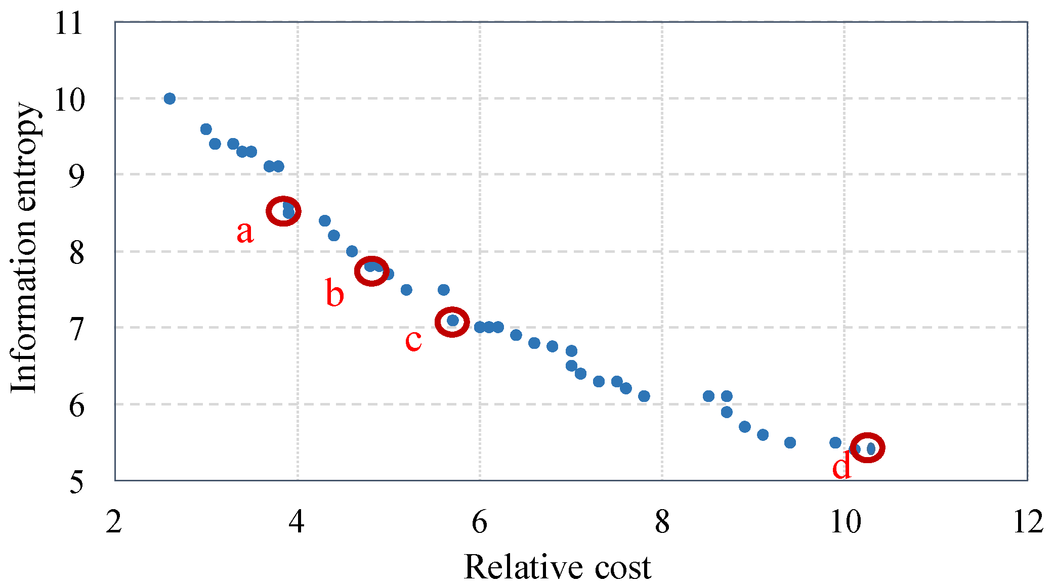
20]. In this paper, an approach that develops Pareto frontier is presented to derive optimal feasible solutions depending on the decision maker’s preference on sensor cost or system information certainty.
A feature of the approach developed herein is the ability to model uncertainties in system model and measurement process. These uncertainties are typically associated with leak location and environmental factors, process conditions, measurement accuracy, etc. The proposed methodology uses Bayesian networks (BNs), integrating representation of the system configuration and information sources, and associated uncertainties. There have been several studies focused on optimizing sensor placement using BN. Flynn et al. [21] define two error types associated with damage detection and use BN to quantify two performance measures of a given sensor configuration. The so called genetic algorithm is used to derive the performance-maximizing configuration. In Li et al. [22] a probabilistic model based on BN is developed that considers load uncertainty and measurement error. The optimal sensor placement is derived by optimizing three distinct utility functions that describe quadratic loss, Shannon information, and Kullback–Leibler divergence. Other studies that focus on BNs include objective functions that describe the minimum probability of errors [23], and the smallest and largest local average log-likelihood ratio [24]. In our study, sensor selection optimization methodology maximizes information metric on system health considering sensor costs. Information entropy quantifies the uncertainty of random variables [25].
Minimizing the information entropy decreases the uncertainty. The effectiveness of any model-based condition monitoring scheme is a function of the magnitude of uncertainty in both the measurements and models [26,27]. In [27], it is demonstrated that uncertainty affects all aspects of system monitoring, modelling, and control, and naturally the identification of the optimal sensor combination. The uncertainty stemming from modelling and sensors should therefore be considered in the optimization procedure.
Uncertainty can be quantified using different metrics. One of the popular metrics of uncertainty quantification is information entropy index. Minimizing the differential entropy decreases the uncertainty or disorder, and hence increases information value [25].
A key feature of the method proposed in this paper is that here the optimization is based on answering the following question: which combination of sensor types and locations provides highest amount of information about the reliability metric of interest (e.g., probability of system failure)? The increase or decrease in information is measured by entropy. As a result, different types of sensors can be compared based on their information value, and the optimal sensor combination identified based on a common metric.
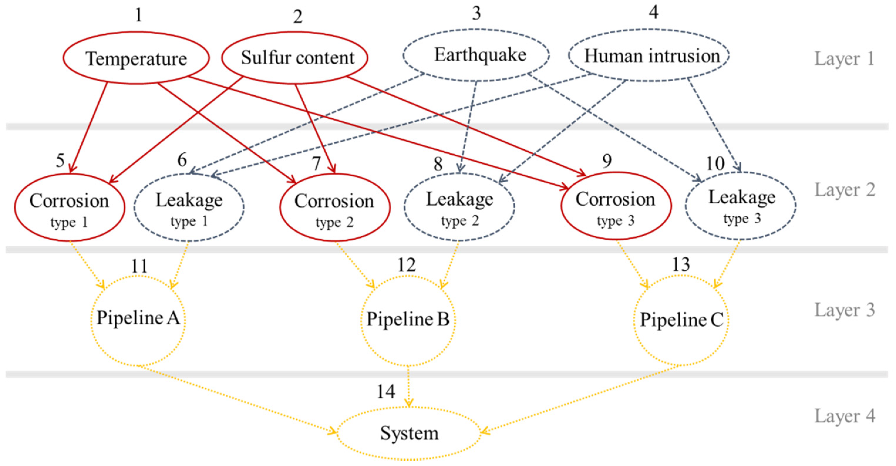
For instance, in a gas pipeline health monitoring context, detectors for temperature, sulfur content, seismic load, human intrusion, corrosion rate, and pipe leakage are compared based on how they change the information on pipe rupture probability (system state), and then the best combination in terms of information gain, considering budget limits, is identified.
We also note that other research presented in Table 1, focus on the placement of one type of sensor, whereas in the present paper considers simultaneous use of different types sensor as part of optimization on information. For example, in [10], contaminant detectors are optimally placed in a water network in order to reduce the detection time and increase the protected population from consuming contaminated water.
In Section 2 of this paper, information entropy as it relates to BNs is explained. The proposed sensor selection model based on BNs is presented in Section 3, and the optimization methodology is described in Section 4. In order to illustrate the proposed methodology, it is applied to a very simple oil pipeline example with key features adequate to demonstrate the method and its results. The network model and results are discussed in Section 5. Finally, the study is concluded with an overall discussion on key advantages of the proposed methodology in Section 6.

2. An Overview of Information Entropy and BNs

Incomplete information and probabilistic representation of information are generally prevalent in system health monitoring applications. Quantification of the uncertainty is one of the primary challenges for measuring the extent to which you have information regarding a system.
In recent years, several authors have investigated uncertainty representation using the concept of entropy and information theory. Information entropy is used to quantify the average uncertainty of an information source. Let X be a random variable with probability distribution of P, where pi is the probability of outcomes x i X . The information content associated with a particular value of this random variable, as defined by the probability distribution can be calculated as Equation (1) [28].
I ( x i ) = log p i
The information function, computes the amount of information (measured in bits) conveyed by a particular state. The expected value of information is the information entropy function H ( X ) , which is calculated by Equation (2).
H ( X ) = E [ I ( X ) ]
The expression for information entropy is developed further in Equation (3) for discrete random variables [28].
H ( X ) = i = 1 n p i × I ( x i ) = i = 1 n p i × log p i
Generalizing to continuous random variables, the information entropy of the random variable X is defined as
H ( X ) = ( f ( x ) × log f ( x ) ) d x
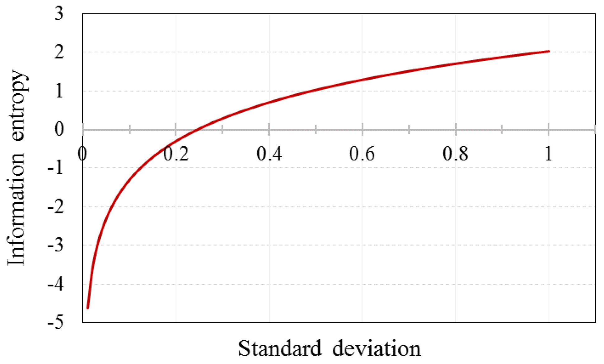
The information entropy increases with respect to the data uncertainty of a random variable. It also increases as the ‘dispersion’ of a random variable increase, as illustrated in Figure 1 for the standard deviation of a normal distribution function f ( x | μ , σ 2 ) .
In methodology proposed below, the distribution of BN (or system) state variables [10] can be constructed by domain experts or synthesized automatically from system operating data. Probability distributions of these state variables convey information uncertainty of the system status. In a BN with single valued probabilities of random variables x i and joint probability, P , given by
P ( x 1 , x 2 , , x n ) = Π i = 1 n p ( x i | y )
the information entropy is calculated from Equation (6), [25,29].
H ( x 1 , x 2 , , x n ) = i = 1 n p ( x i ) × log p ( x i )

3. Sensor Selection Optimization Based on Information Entropy in BNs

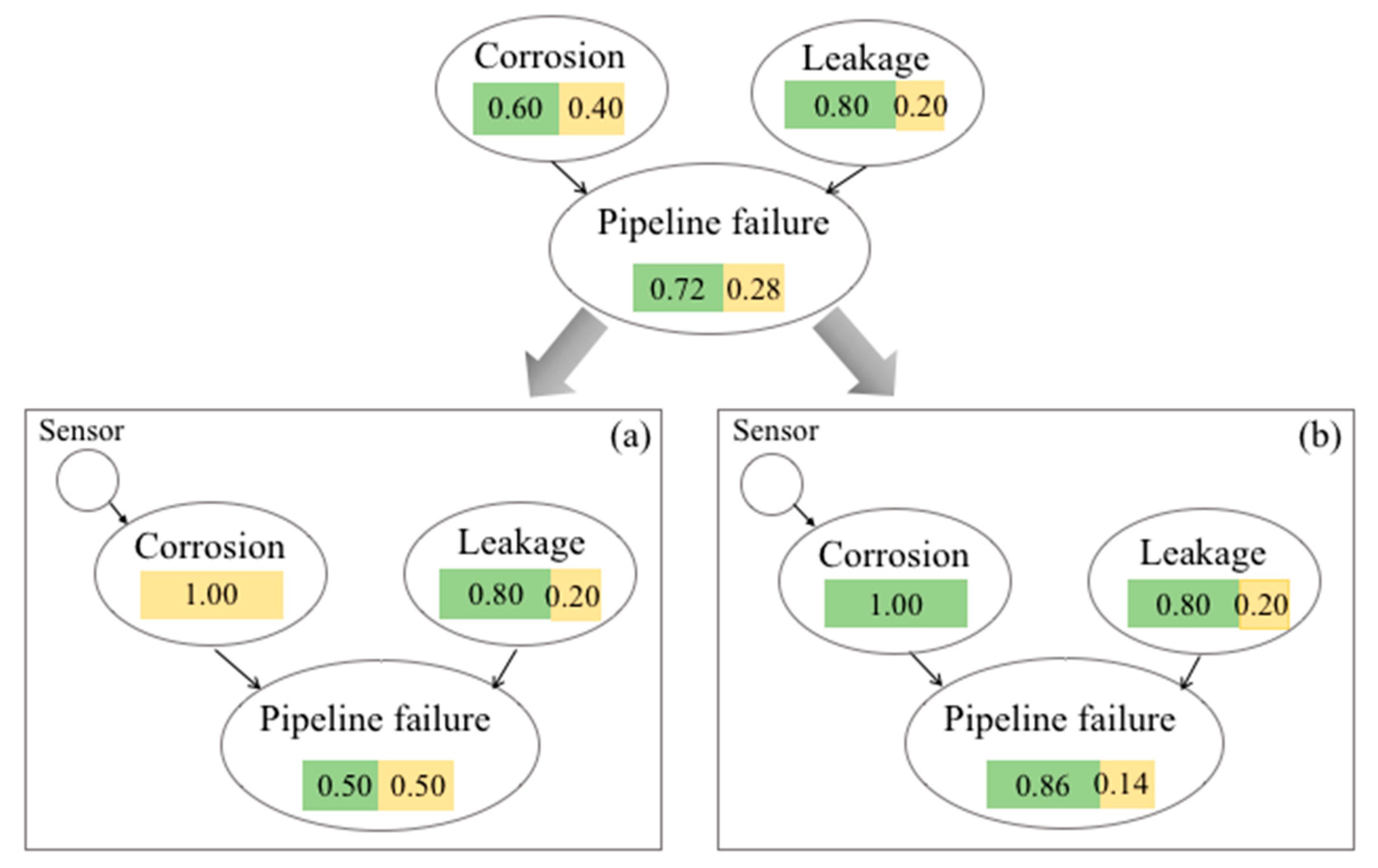
The assessment of system health and condition is based on our understanding of the BN node state variables, which are represented by their joint probability distributions. Figure 2 illustrates the inference engine of a simple three-node BN in which each node has two states: success (green) and failure (yellow). The joint probabilities of this network are presented in Table 2.
According to Table 2, the failure probability of the pipeline node can be calculated as
P ( f ) = P ( f | n c . n l ) × P ( n c ) × P ( n l ) + P ( f | n c . l ) × P ( n c ) × P ( l )   + P ( f | c . n l ) × P ( c ) × P ( n l ) + P ( f | c . l ) × P ( c ) × P ( l ) = 0.10 × 0.60 × 0.80 + 0.30 × 0.60 × 0.20 + 0.40 × 0.40 × 0.80 + 0.90 × 0.40 × 0.20 = 0.28
The probability of the safe state of pipeline node is then equal to P ( s ) = 1 P ( f ) = 0.72 , which is presented in Figure 2 with a green box.
As a sensor is placed on a node, the posterior probability distribution of BN state variables can be computed using evidence nodes. Evidence contains information regarding a set of random variables, and the posterior probability of monitored state x e of an evidence node is equal to one at the observed value.
p ( x e * ) = 1
For instance, in Figure 2, sensor on corrosion node updates the probabilities of this node. The sensor can detect two states of ‘corrosion’ (Scenario (a)) and ‘no corrosion’ (Scenario (b)) in the pipeline. For instance, in Scenario (a), the probability of corrosion is updated to 1, and the probability of no corrosion state is updated to 0, as presented in Figure 2a. Consequently, the posterior probability distribution of BN states is updated.
In this paper, placing a sensor at a particular place in a system makes the corresponding node an evidence node. Moreover, it is assumed that the sensor reports all states of the evidence node. Therefore, total system information entropy can be calculated based on the probability distribution of the state of the evidence node as shown in Equation (9)
H ( x ) = k = 1 k * ( p k × j = 1 m i = 1 n j p ( x i j k ) × log p ( x i j k ) )
Here, n j is the number of node states, m is the number of BN nodes and k * is the number of possible evidence observations scenarios based on selected sensor and p k is its probability.
Based on the prior knowledge of the state variables’ probability distribution, the total system information entropy is 0.77, which is equal to the sum of the all individual node information entropies.
H ( x ) = j = 1 3 i = 1 2 p ( x i j a ) . log p ( x i j a ) = 0.60 × log 0.60 + 0.40 × log 0.40 + 0.80 × log 0.80 + 0.20 × log 0.20 + 0.72 × log 0.72 + 0.28 × log 0.28 = 0.77
By placing a sensor on the corrosion node, the system information entropy is calculated using all possible sensor observations (evidence). In the example below, possible sensor evidence observations are two scenarios (a) and (b), and the total system information entropy would be 0.44
H ( x ) = p a j = 1 3 i = 1 2 p ( x i j a ) log p ( x i j a ) p b j = 1 3 i = 1 2 p ( x i j b ) log p ( x i j b ) = 0.40 × 0.52 + 0.60 × 0.39 = 0.44
As can be seen, corrosion node has two states. Therefore, two evidence observation scenarios are possible. Scenario (a) is the failure state of the corrosion node (sensor does not detect corrosion) and scenario (b) is its success (sensor detects corrosion). In Equation (11), p a and p b are the prior probabilities of corrosion node states for (a) and (b) scenarios, respectively.

3.1. Information Value

In the example of Figure 2, it is assumed that information associated with all nodes have the same weight (value). The weight of a node information reflects the extent to which it informs a subsequent decision, or yields value to an organization or activity, such as the modification of inspection plan. In most cases, the expected cost of failure of different system elements (represented by BN nodes) are not identical. Consequently, the information entropy importance of different nodes would not be equal. To accommodate such situations, information entropy of each node can be weighted via Equation (12).
w j = m ( expected   cost   of   failure ) j j = 1 m expected   cost   of   failure
where m is the number of nodes with different information value. The weights sum to one. The total system information entropy is then calculated using Equation (13).
H ( x ) = k = 1 k * ( p k × j = 1 m w j × i = 1 n p ( x i j k ) × log p ( x i j k ) )

3.2. Sensor Reliability and Measurement Uncertainty

BN state variable probability distributions are continually updated using sensor data, noting that they can be uncertain [25]. This uncertainty may be inherent to the process of gathering data (condition variability and human observation uncertainty) or it may stem from the sensor uncertainty. To consider these uncertainties, sensors can be represent as ‘soft evidence’ nodes, which carry two additional piece of information: the operational mode and the probability of its occurrence [30].
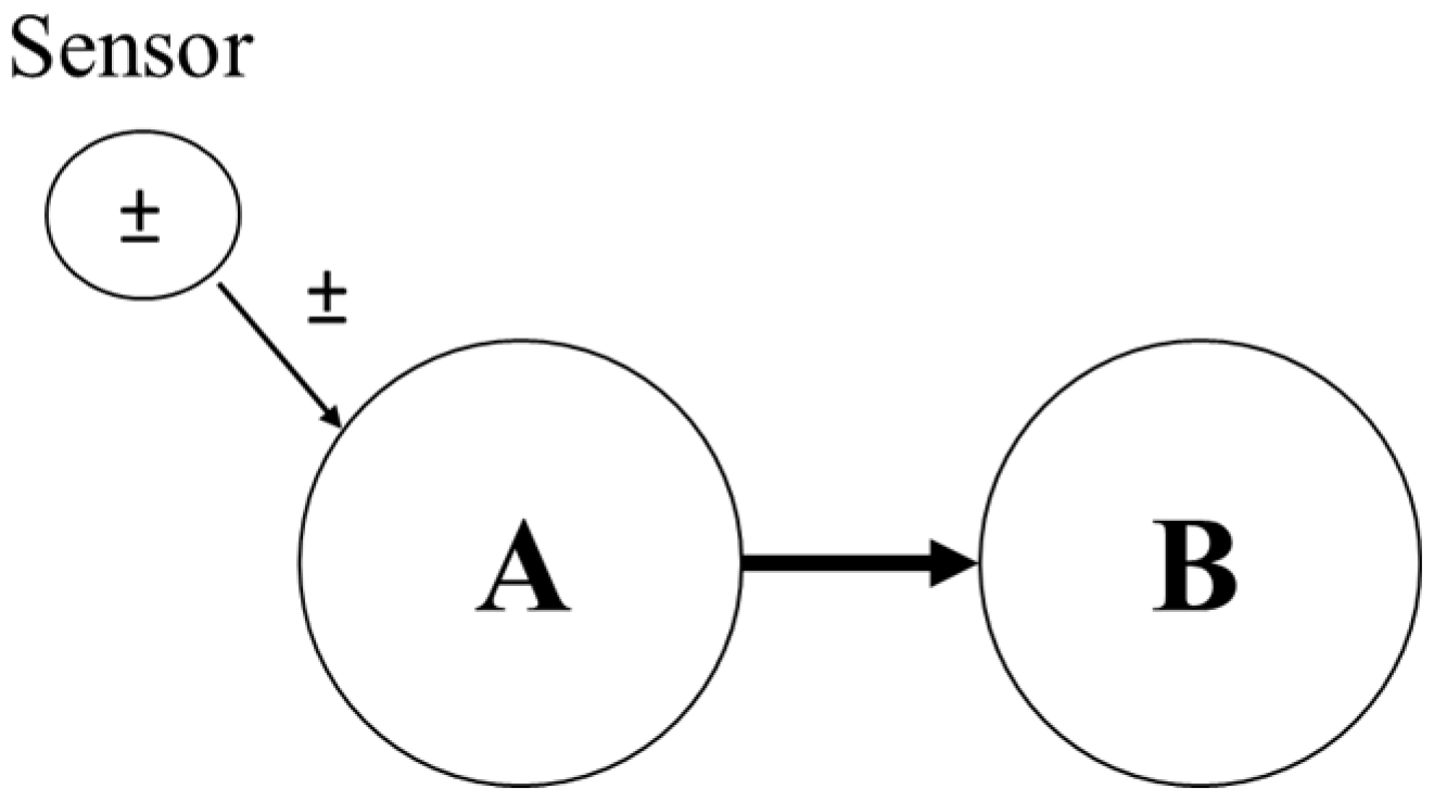
The state of knowledge about BN ‘soft evidence’ nodes are usually modelled by probability distributions using Jeffrey’s rule [29]. The posterior probability of node B’s state variable presented in Figure 3 is defined as
P ( B ) = i P ( B | A i ) × P ( A | S i )
where, P ( A | S ) is the conditional probability of A given ‘soft evidence’, and P ( B | A ) is the conditional probability of B given A, before evidence.

4. Optimization Methodology

4.1. Problem Formulation

The sensor selection optimization problem involves the competing goals of maximizing information, minimizing sensors cost, and optimizing physical constraints (such as size and weight limitations). In an m node BN with T j possible sensor types for the j-th node under consideration, and M T j models for the sensor type T j , the number of possible sensor selection combinations is
j = 1 m ( T j × M T j + 1 )
The multi-objective optimization approach used herein is based on an objective function that contains two weighted indices representing sensor cost and information entropy as described in Equation (16).
M i n   [ ω 1 × C ( y ) + ω 2 × H ( y ) ]
where C ( y ) is the cost of a particular sensor configuration, H(y) is system information entropy, and ω 1 , ω 2 are the weighting factors of the cost and system information entropy, respectively. Using weight values is one of the methods for transforming multi-objective to single-objective problems. In this approach, different weight values are considered, and a different solution is derived for each of the used weights. Pareto front is then obtained based on combination of these solutions.
The objective function can be subject to several constraints. For instance, Equation (17) imposes a limitation on budget or total sensor cost, and Equation (18) imposes a minimum acceptable level of system health information.
C ( y ) C max
I ( y ) I min

4.2. Solution Approach

A multi objective optimization problem usually has a set of solutions that is known as the Pareto-optimal set. Each Pareto optimal solution in an optimal set which represents a compromise between objective functions, acknowledging that the objective functions cannot be all simultaneously improved. Different solution approaches, including exact and heuristic, have been proposed to solve multi-objective optimization problems once the multi-objective problem is transformed into single objective case. Linear or small size problems can be solved using exact solution algorithms. These algorithms include gradient search method, dynamic programming, and branch-and-bound algorithm which is mainly used in linear mixed-integer problems. Heuristic methods such as artificial bee evolutionary programming (EP), genetic algorithm (GA), and particle swarm optimization (PSO) are generally used for larger or nonlinear problems [31,32].
The most commonly used heuristic methods are population-based evolutionary techniques that are inspired by evolution in nature. The subject now includes GA and PSO. These algorithms stem from the very basic description of biological systems. Evolutionary techniques are classified as stochastic search algorithms for global optimization problems, which have found many engineering and industrial applications. The GA and PSO algorithms have been compared in [33]. Results indicate that PSO is more computationally efficient as it uses fewer number of function evaluations.
PSO is inspired by simulations of social behaviors. PSO shares many similarities with evolutionary computation techniques such as GAs, including initialization with a population of random solutions and search for optima by updating generations. However, unlike GA, PSO has no evolution operators such as crossover and mutation. In PSO, potential solutions, called particles, fly through a problem space by following the current optimum particles. In general, compared with GAs, the advantages of PSO is that it is easy to implement and there are few parameters to adjust. Recent studies of PSO indicate that although the standard PSO outperforms other EAs in early iterations, it does not improve the quality of solutions as the number of generations is increased. This means that it can converge with fewer iterations, and as a result the solution time is shorter that other EAs [34,35].
The proposed optimization model in this study is an integer nonlinear problem. The PSO method is a better solution approach for this problem in comparison with other algorithms due to its simplicity of calculations, not needing mutation and overlapping calculations, and high speed of convergence in nonlinear optimization problems [35,36]. Figure 4 depicts the data flow diagram of the developed integer multi objective particle swarm optimization (IMOPSO) algorithm that can be used in sensor selection optimization problems based on BNs. The IMOPSO algorithm randomly initializes or creates a population of state variable sets. Each state variable set is called a ‘particle’ Y = [ y ( 1 ) , y ( 2 ) , , y ( m ) ] in which y ( j ) is the j-th node’s state variable (sensor status). Including sensor existence, sensor types T j , and models M T j . The particle moves through the solution space following some basic formulae in search of a global optimum. The velocity of each particle V = [ v ( 1 ) , v ( 2 ) , , v ( m ) ] at each generation of movement changes based on the last optimum particles [37]. After several generations, only the ‘most optimal’ particles can transmit information to other particles, making the optimization very fast in comparison to other evolutionary techniques [38,39].

5. Application Example and Numerical Evaluation

In the following, the proposed methodology is illustrated with a very simple example that has the key characteristics to show how the technique works and what types of results could be expected.

5.1. Problem Statement

The problem to be addressed is sensor selection in an oil pipeline network. The pipeline is divided into three segments with different characteristics. The general structure of the three-segment pipeline and a corresponding fault tree are illustrated in Figure 5a,b, respectively.
The fault tree gates are mapped into the BN and event likelihoods are defined using a conditional probability table. Figure 6 shows a four-layer BN of the exemplar oil pipeline network. The first layer of nodes are external causes of system degradation, here ambient temperature, chemical content, earthquake shock, and human intrusion. The second layer nodes primarily consist of corrosion and leakage. The failure mechanisms are assumed to be independent. The third layer presents the health status nodes of the three pipeline segments.
Table 3 and Table 4 are examples of the conditional probability tables for corrosion mechanism.
The effect of sensor uncertainties is considered in the proposed Bayesian model by assuming that all nodes are soft nodes which are inherently uncertain. Therefore, the reliability of the sensor, which is highly dependent on its cost, is assumed to affect the information certainty. Table 5 presents sensors relative cost and reliability in the studied case.

5.2. Results and Discussion

The population size, maximum number of iterations, and size of the external repository should be determined for the proposed IMOPSO algorithm. In general, the population size and number of iterations have an inverse relation, as a smaller population size requires higher number of iterations and vice versa. In this study, a population size of 50 is used and the maximum number of iterations is guided by convergence of the results. In addition, the maximum size of repository is set to 100 and a variable-size repository is initially set to 5% of maximum size of repository, and then increased in a stepwise manner until it reaches the maximum size of repository. The results converge well when repository of 50 is used. Figure 7 is the Pareto frontier of locally optimum sensor selection. Each point on the curve has no other sensor combinations where both cost and entropy are better.
As illustrated in Figure 7, relative cost ranges between 2.6 and 10.5 corresponding to information entropy ranging between 5.4 and 10. The range of Pareto optimal solutions along the Pareto frontier provides the decision maker ample flexibility to identify an optimum cost-effective combination, while maintaining acceptable system information entropy. Further, the Pareto frontier illustrates the relationship between marginal information entropy and relative cost at optimum sensor combination.
Table 6 describes selected optimal sensor combinations on the Pareto frontier illustrated in Figure 7. As can be seen, higher budgets permit higher reliability (Model 3 rather than 2 or 1).
Figure 8 illustrates the selected optimal sensor locations (from Figure 7 and Table 6) with respect to the BN. It can be seen that the optimization methodology preferences sensors at the third layer.
The optimization process up until this point has assumed that the information about each of three pipeline segments have the same value. This may not be the case in practice. For example, one pipe segment may have greater difficulties associated with maintenance crew access, making failure more expensive. To make the optimization more robust, information value can be weighted based on failure cost, which will be a function of both reliability and repair cost.
Key statistics (in the form of percentiles) of the resultant segment failure frequencies of pipeline segments are presented in Table 7. It can be seen that segment A is the least reliable, followed by segments B and C, respectively.
Taking into account the failure cost of individual pipe segments, the ‘rank’ of segment importance changes as seen in Table 8.
The coefficient weight of information entropy of each node can be calculated from Equation (10), and system total entropy is evaluated based Equation (19).
H ( x ) = k = 1 r ( p k × ( j = 1 10 i = 1 n H i j k + 1.79 × i = 1 n H i 11 k + 0.56 × i = 1 n H i 12 k + 0.65 × i = 1 n H i 13 k + i = 1 n H i 14 k ) )
Figure 9 illustrates the Pareto front considering information value of pipeline segments in the optimization procedure.
The selected optimal combinations on the Pareto front are presented in Table 9.
The selected optimal sensor combinations are illustrated as they relate to the BN in Figure 10. As can be seen, the optimal combinations differ from Figure 8. In this scenario, sensors are placed reflecting information value of each node, and consequently as is shown, the minimum number of sensors tend to be those that provide more information about node 11 (pipeline A), followed by node 13 (pipeline C). This reflects the ‘importance rank’ from Table 8.

6. Concluding Remarks

Optimal sensor selection for system health monitoring is a generally well explored problem in industrial systems, but there is scope for it to be developed further. This paper proposes a new methodology for sensor selection optimization based on information gain and sensor cost. The novelty of the methodology lies in the application of the information entropy using BN model of the system and information sources in a way that incorporates sensor and measurement uncertainties. The developed methodology is illustrated using a very simple oil pipeline network, producing several optimal sensor combinations. The PSO algorithm was used to solve the multi-objective optimization problem, producing a Pareto frontier. Results show that the proposed methodology is effective in sensor selection optimization problems with multiple criteria that involve uncertainty. Furthermore, the information value of Bayesian nodes is weighted regarding nodes failure costs, and results indicate that sensor optimal combinations are highly affected by weighting information value.

Author Contributions

A.M. conceived of the presented idea and developed the theory. S.B. encouraged T.P. to quantify the uncertainty of the systems’ health information using entropy concept. T.P. performed the computations and verified the analytical method. A.M. supervised the findings of this work. All authors discussed the results and contributed to the final manuscript.

Acknowledgments

This work received support from the Pipeline System Integrity Management Project, sponsored by the Petroleum Institute, Abu Dhabi, United Arab Emirates.

Conflicts of Interest

The authors declare no conflict of interest in relation to the content of this paper.

References

  1. Bhuiyan, M.Z.A.; Wang, G.; Cao, J.; Wu, J. Sensor Placement with Multiple Objectives for Structural Health Monitoring. ACM Trans. Sens. Netw. 2014, 10, 1–45. [Google Scholar] [CrossRef]
  2. Pino-Povedano, S.; González-Serrano, F.J. Comparison of Optimization Algorithms in the Sensor Selection for Predictive Target Tracking. Ad Hoc Netw. 2014, 20, 182–192. [Google Scholar] [CrossRef]
  3. Zhao, Y.; Schwartz, R.; Salomons, E.; Ostfeld, A.; Vincentpoor, H. New Formulation and Optimization Methods for Water Sensor Placement. Environ. Model. Softw. 2016, 76, 128–136. [Google Scholar] [CrossRef]
  4. Ramsden, D. Optimization Approaches to Sensor Placement Problems. Ph.D. Thesis, Graduate Faculty of Rensselaer Polytechnic Institute Troy, New York, NY, USA, 2009. [Google Scholar]
  5. Guo, Y.; Kong, F.; Zhu, D.; Tosun, A.S.; Deng, Q. Sensor Placement for Lifetime Maximization in Monitoring Oil Pipelines. In Proceedings of the 1st ACM/IEEE International Conference on Cyber-Physical Systems (ICCPS ’10), Stockholm, Sweden, 13–15 April 2010; ACM: New York, NY, USA, 2010; pp. 61–68. [Google Scholar]
  6. Xia, C.; Liu, W.; Deng, Q. Cost Minimization of Wireless Sensor Networks with Unlimited-lifetime Energy for Monitoring Oil Pipelines. IEEE/CAA J. Autom. Sin. 2015, 2, 290–295. [Google Scholar]
  7. Legg, S.W.; Wang, C.; Benavides-Serrano, A.J.; Laird, C.D. Optimal Gas Detector Placement under Uncertainty Considering. J. Loss Prev. Process Ind. 2013, 26, 410–417. [Google Scholar] [CrossRef]
  8. Elnaggar, O.E.; Ramadan, R.A.; Fayek, M.B. WSN in Monitoring Oil Pipelines Using ACO and GA. Procedia Comput. Sci. 2015, 52, 1198–1205. [Google Scholar] [CrossRef]
  9. Li, H.; Yao, T.; Ren, M.; Rong, J.; Liu, Ch.; Jia, L. Physical Topology Optimization of Infrastructure Health Monitoring Sensor Network for High-Speed Rail. Measurement 2016, 79, 83–93. [Google Scholar] [CrossRef]
  10. Krause, A.; Leskovec, J.; Guestrin, C.; VanBriesen, J.; Faloutsos, C. Efficient Sensor Placement Optimization for Securing Large Water Distribution Networks. J. Water Resour. Plan. Manag. 2008, 134, 516–527. [Google Scholar] [CrossRef]
  11. Pourali, M.; Mosleh, A. A Bayesian Approach to Online System Health Monitoring. In Proceedings of the Reliability and Maintainability Annual Symposiu (RAMS), Orlando, FL, USA, 28–31 January 2013; pp. 210–215. [Google Scholar]
  12. Pourali, M.; Mosleh, A. A Functional Sensor Placement Optimization Method for Power Systems Health Monitoring. IEEE Trans. Ind. Appl. 2013, 49, 1711–1719. [Google Scholar] [CrossRef]
  13. Rico-Ramirez, V.; Frausto-Hernandez, S.; Diwekar, U.M.; Hernandez-Castro, S. Water Networks Security: A Two-Stage Mixed-Integer Stochastic Program for Sensor Placement under Uncertainty. Comput. Chem. Eng. 2007, 31, 565–573. [Google Scholar] [CrossRef]
  14. Lam, H.F.; Yang, J.H.; Hu, Q. How to Install Sensors for Structural Model Updating? Procedia Eng. 2011, 14, 450–459. [Google Scholar] [CrossRef]
  15. Antoniades, C.; Christofides, P.D. Integrated Optimal Actuator/Sensor Placement and Robust Control of Uncertain Transport-Reaction Processes. Comput. Chem. Eng. 2002, 26, 187–203. [Google Scholar] [CrossRef]
  16. Almeidaa, M.D.; Costa, F.F.; Xavier-de-Souzac, S.; Santana, F. Optimal Placement of Faulted Circuit Indicators in Power Distribution Systems. Electr. Power Syst. Res. 2011, 81, 699–706. [Google Scholar] [CrossRef]
  17. Weickgenannt, M.; Neuhaeuser, S.; Henke, B.; Sobek, W.; Sawodny, O. Optimal Sensor Placement for State Estimation of A Thin Double-Curved Shell Structure. Mechatronics 2013, 23, 346–354. [Google Scholar] [CrossRef]
  18. Fei, X.; Mahmassani, H.S.; Murray-Tuite, P. Vehicular Network Sensor Placement Optimization under Uncertainty. Transp. Res. Part C Emerg. Technol. 2013, 29, 14–31. [Google Scholar] [CrossRef]
  19. Domingo-Perez, F.; Lazaro-Galilea, J.L.; Wieser, A.; Martin-Gorostiza, E.; Salido-Monzua, D.; Llana, A. Sensor Placement Determination for Range-Difference Positioning Using Evolutionary Multi-Objective Optimization. Expert Syst. Appl. 2016, 47, 95–105. [Google Scholar] [CrossRef]
  20. Wang, Y.; Li, H.X.; Yen, G.G.; Song, W. MOMMOP: Multi-objective Optimization for Locating Multiple Optimal Solutions of Multimodal Optimization Problems. IEEE Trans. Cybern. 2015, 45, 830–843. [Google Scholar] [CrossRef] [PubMed]
  21. Flynn, E.B.; Michael, D.T. A Bayesian Approach to Optimal Sensor Placement for Structural Health Monitoring with Application to Active Sensing. Mech. Syst. Signal Process. 2010, 24, 891–903. [Google Scholar] [CrossRef]
  22. Li, B.; Kiureghian, A.D. Robust Optimal Sensor Placement for Operational Modal Analysis Based on Maximum Expected Utility. Mech. Syst. Signal Process. 2016, 75, 155–175. [Google Scholar] [CrossRef]
  23. Zhao, Y.; Chen, J.; Goldsmith, A.; VincentPoor, H. Identification of Outages in Power Systems with Uncertain States and Optimal Sensor Locations. IEEE J. Sel. Top. Signal Process. 2014, 8, 1140–1153. [Google Scholar] [CrossRef]
  24. Chepuri, S.P.; Leus, G. Sparse Sensing for Distributed Detection. IEEE Trans. Signal Process. 2016, 64, 1446–1460. [Google Scholar] [CrossRef]
  25. Pourali, M. A Bayesian Approach to Sensor Placement Optimization and System Health Monitoring. Ph.D. Thesis, Centre for Risk and Reliability, A. James Clark School of Engineering, University of Maryland, College Park, MD, USA, 2013. [Google Scholar]
  26. Buswell, R.A. Uncertainty in the First Principle Model-Based Condition Monitoring of HVAC Systems. Ph.D. Thesis, Loughborough University, Leicestershire, UK, 2001. [Google Scholar]
  27. Buswell, R.A.; Wright, J.A. Uncertainty in model-based condition monitoring. Build. Serv. Eng. Res. Technol. 2004, 25, 65–75. [Google Scholar] [CrossRef]
  28. Gray, R.M. Entropy and Information Theory, 1st ed.; Springer: New York, NY, USA, 2013. [Google Scholar]
  29. Peng, Y.; Zhang, S.; Pan, R. Bayesian Network Reasoning with Uncertain Evidences. Int. J. Uncertain. Fuzziness Knowl.-Based Syst. 2010, 18, 539–564. [Google Scholar] [CrossRef]
  30. Mrad, A.B.; Delcroix, V.; Maalej, M.A.; Piechowiak, S.; Abrid, M. Advances in Computational Intelligence, Uncertain Evidence in Bayesian Networks: Presentation and Comparison on a Simple Example. In Computer and Information Science; Springer: Berlin/Heidelberg, Germany, 2012; Volume 299, pp. 39–48. ISBN 976-3-642-31718-7. [Google Scholar]
  31. Cabadag, R.İ.; Turkay, B.E. Heuristic methods to solve optimal power flow Problem. IU-J. Electr. Electron. Eng. 2013, 13, 1653–1659. [Google Scholar]
  32. Simon, D. Evolutionary Optimization Algorithms; Wiley: New York, NY, USA, 2013; ISBN 978-0470-93741-9. [Google Scholar]
  33. Hassan, R.; Cohanim, B.; de Weck, O.; Venter, G. A Comparison of Particle Swarm Optimization and the Genetic Algorithm; American Institute of Aeronautics and Astronautics: Reston, VA, USA, 2004. [Google Scholar]
  34. Tang, W.H.; Wu, Q.H. Chapter 2. Evolutionary Computation, Condition Monitoring and Assessment of Power Transformers Using Computational Intelligence; Springer Science & Business Media: Berlin/Heidelberg, Germany, 2011. [Google Scholar]
  35. Jancauskas, V. Evaluating the Performance of Multi-Objective Particle Swarm Optimization Algorithms, Ph.D. Thesis, Vilnius University, Vilnius, Lithuania, 2016. [Google Scholar]
  36. Wang, D.; Tan, D.; Liu, L. Particle swarm optimization algorithm: An overview. Soft Comput. 2018, 22, 387–408. [Google Scholar] [CrossRef]
  37. Clerc, M. Particle Swarm Optimization; Wiley: New York, NY, USA, 2013; ISBN 978-1-118-61397-9. [Google Scholar]
  38. Yu, B.; Yuanping, W.; Liang, Z.; Yuan, H.; Aijuan, Z. Relay Node Deployment for Wireless Sensor Networks Based on PSO. In Proceedings of the IEEE International Conference on Computer and Information Technology, Ubiquitous Computing and Communications, Liverpool, UK, 26–28 October 2015. [Google Scholar]
  39. Farzinfar, M.; Jazaeri, M.; Razavi, F. A New Approach for Optimal Coordination of Distance and Directional Over-Current Relays Using Multiple Embedded Crossover PSO. Int. J. Electr. Power Energy Syst. 2014, 61, 620–628. [Google Scholar] [CrossRef]
  40. Dawotola, A.W.; Gelder, P.H.A.J.M.; Vrijling, J.K. Decision Analysis Framework for Risk Management of Crude Oil Pipeline System. Adv. Decis. Sci. 2011, 2011, 456824. [Google Scholar] [CrossRef]
Figure 1. Information entropy as a function of dispersion for a normally distributed variable.
Entropy 20 00416 g001
Figure 2. BN evidence scenarios with corrosion sensor. (a) no corrosion; (b) corrosion.
Entropy 20 00416 g002
Figure 3. Considering sensor as a soft evidence in BN.
Entropy 20 00416 g003
Figure 4. Data flow of sensor selection optimization procedure based on IMOPSO.
Entropy 20 00416 g004
Figure 5. (a) Studied oil pipeline schematic; (b) fault tree of the pipeline.
Entropy 20 00416 g005
Figure 6. BN of the studied oil pipeline network.
Entropy 20 00416 g006
Figure 7. Pareto front of optimal sensor combinations.
Entropy 20 00416 g007
Figure 8. Optimal sensor combinations of selected optimal scenarios. (a) Scenario a; (b) Scenario b; (c) Scenario c; (d) Scenario d.
Entropy 20 00416 g008
Figure 9. Pareto frontier of locally optimal sensor combinations.
Entropy 20 00416 g009
Figure 10. Optimal sensor combinations of selected optimal scenarios considering information value. (a) Scenario a; (b) Scenario b; (c) Scenario c; (d) Scenario d.
Entropy 20 00416 g010
Table 1. Sensor placement optimization literature summary.
Objective FunctionLinearityUncertaintySolution MethodSystem under StudyRef.
SingleLinearNot consideredCutting-plane approach, semi-definite programming approachFramework[4]
SingleLinearNot consideredMixed integer linear programming solverOil Pipeline[5]
SingleLinearNot consideredWorst case energy balance strategyOil Pipeline[6]
SingleLinearConsideredCPLEXGas detector[7]
SingleNonlinearNot consideredGenetic algorithm, ant colony algorithmOil Pipeline[8]
SingleNonlinearNot consideredDynamic programming, simulated annealing, Particle swarm optimization algorithm, ant colony optimization algorithmHigh-speed rail[9]
MultiNonlinearNot consideredGreedy algorithmWater network[10]
SingleNonlinearConsideredBayesian approachFramework[11]
SingleNonlinearConsideredBayesian approachFramework[12]
SingleNonlinearConsideredStochastic decomposition algorithmWater network[13]
SingleNonlinearConsideredBayesian approach, genetic algorithmFramework[14]
SingleNonlinearConsideredGradient search methodTransport-reaction process[15]
SingleNonlinearConsideredGenetic algorithmPower distribution system[16]
MultiNonlinearConsideredAnnealing algorithmShell structure[17]
MultiNonlinearConsideredHybrid greedy randomized adaptive search procedureVehicular network[18]
MultiNonlinearConsideredGenetic algorithmFramework[19]
Table 2. Joint probabilities of the BN presented in Figure 2.
StateProbability
P (   f a i l u r e |   n o   c o r r o s i o n ,   n o   l e a k a g e ) = P ( f | n c , n l ) 0.10
P (   f a i l u r e |   n o   c o r r o s i o n ,   l e a k a g e ) = P ( f | n c , l ) 0.70
P (   f a i l u r e |   c o r r o s i o n ,   n o   l e a k a g e ) = P ( f | c , n l ) 0.60
P (   f a i l u r e |   c o r r o s i o n ,   l e a k a g e ) = P ( f | c , l ) 0.90
Table 3. An example of the conditional probability table for corrosion mechanism.
Temperature (Celsius)H2S (ppm)Corrosion Pipeline ACorrosion Pipeline BCorrosion Pipeline C
YesNoYesNoYesNo
20–400–10000.30.70.10.90.20.8
20–401000–10,0000.40.60.20.80.30.7
40–600–10000.350.650.30.70.40.6
40–601000–10,0000.450.550.70.30.80.2
60–800–10000.40.60.60.40.70.3
60–801000–10,0000.70.30.80.20.90.1
80–1000–10000.450.550.30.70.40.6
80–1001000–10,0000.80.20.70.30.80.2
Table 4. An example of the conditional probability table for leakage.
Earthquake (Richter)Human Intrusion (kJ)Leakage Pipeline ALeakage Pipeline BLeakage Pipeline C
YesNoYesNoYesNo
3–40–100.30.70.20.80.10.9
3–4>100.70.30.60.40.50.5
4–50–100.750.250.70.30.650.35
4–5>100.80.20.70.30.60.4
5–60–100.850.150.80.20.750.25
5–6>100.950.050.90.10.850.15
Table 5. Reliability and relative cost of sensors.
Node NumberSensor TypeSensor ModelReliabilityRelative Cost
1Temperature10.850.5
20.90.7
30.950.9
2Sulphur detector10.850.5
20.90.7
30.950.9
3Earthquake detector10.850.5
20.90.7
30.950.9
4Human intrusion detector10.850.5
20.90.7
30.950.9
5Corrosion detector10.850.5
20.90.7
30.950.9
6Leakage detector10.850.5
20.90.7
30.950.9
7Corrosion detector10.850.5
20.90.7
30.950.9
8Leakage detector10.850.5
20.90.7
30.950.9
9Corrosion detector10.850.5
20.90.7
30.950.9
10Leakage detector10.850.5
20.90.7
30.950.9
11Failure detector of pipeline A10.850.5
20.90.7
30.950.9
12Failure detector of pipeline B10.850.5
20.90.7
30.950.9
13Failure detector of pipeline C10.850.5
20.90.7
30.950.9
Table 6. Selected optimal combinations on the Pareto front.
No.Information EntropyRelative CostSensors Combination (Sensor, Model)Information Uncertainty
a8.63.9(2, 2), (10, 2), (11, 2), (12, 3), (13, 3)0.31
b7.84.8(2, 2), (6, 2), (10, 2), (11, 3), (12, 3), (13, 3)0.305
c7.15.7(2, 3), (3, 1), (6, 3), (10, 2), (11, 3), (12, 3), (13, 3)0.298
d5.210.5(1, 1), (2, 3), (3, 3), (4, 2), (5, 2), (6, 3), (7, 3), (8, 3), (9, 3), (10, 1), (11, 3), (12, 3), (13, 3)0.285
Table 7. Failure frequencies of three segments (per km·year) [40].
5%50%95%
Pipeline A4.6× 10−42.28 × 10−310.66 × 10⁻³
Pipeline B1.82 × 10−41.75 × 10−37.95 × 10−3
Pipeline C1.47 × 10−41.73 × 10−35.97 × 10−3
Table 8. Expected cost of failure and information value rank of three segments [40].
Pipeline SegmentFailure Cost ($K)Expected Annual Cost of Failure ($K/km·year)Rank
Pipeline A510011.61
Pipeline B20953.673
Pipeline C24254.22
Table 9. Selected optimal combinations on the Pareto front.
No.Information EntropyRelative CostSensors Combinations (Sensor, Model)Information Uncertainty
a9.42.9(1, 1), (3, 1), (5,2), (10, 1), (11, 2)0.318
b6.86.3(1, 1), (2, 2), (3,1), (5, 1), (6, 2), (7, 3), (10, 2), (11, 3), (13, 3)0.295
c6.46.7(1, 1), (2, 2), (3, 1), (5, 1), (6, 3), (7, 3), (10, 3), (11, 3), (13, 3)0.291
d4.89.8(1, 1), (2, 3), (3, 1), (4, 2), (5, 3), (6, 3), (7, 3), (8, 3), (9,3), (10, 3), (11, 3), (13, 3)0.280

