KL Divergence-Based Fuzzy Cluster Ensemble for Image Segmentation


Abstract
:1. Introduction
2. Related Work
2.1. Fuzzy C-Means
2.2. Local Spatial Fuzzy C-Means
2.3. Cluster Ensemble
3. KL Divergence-Based Fuzzy Cluster Ensemble
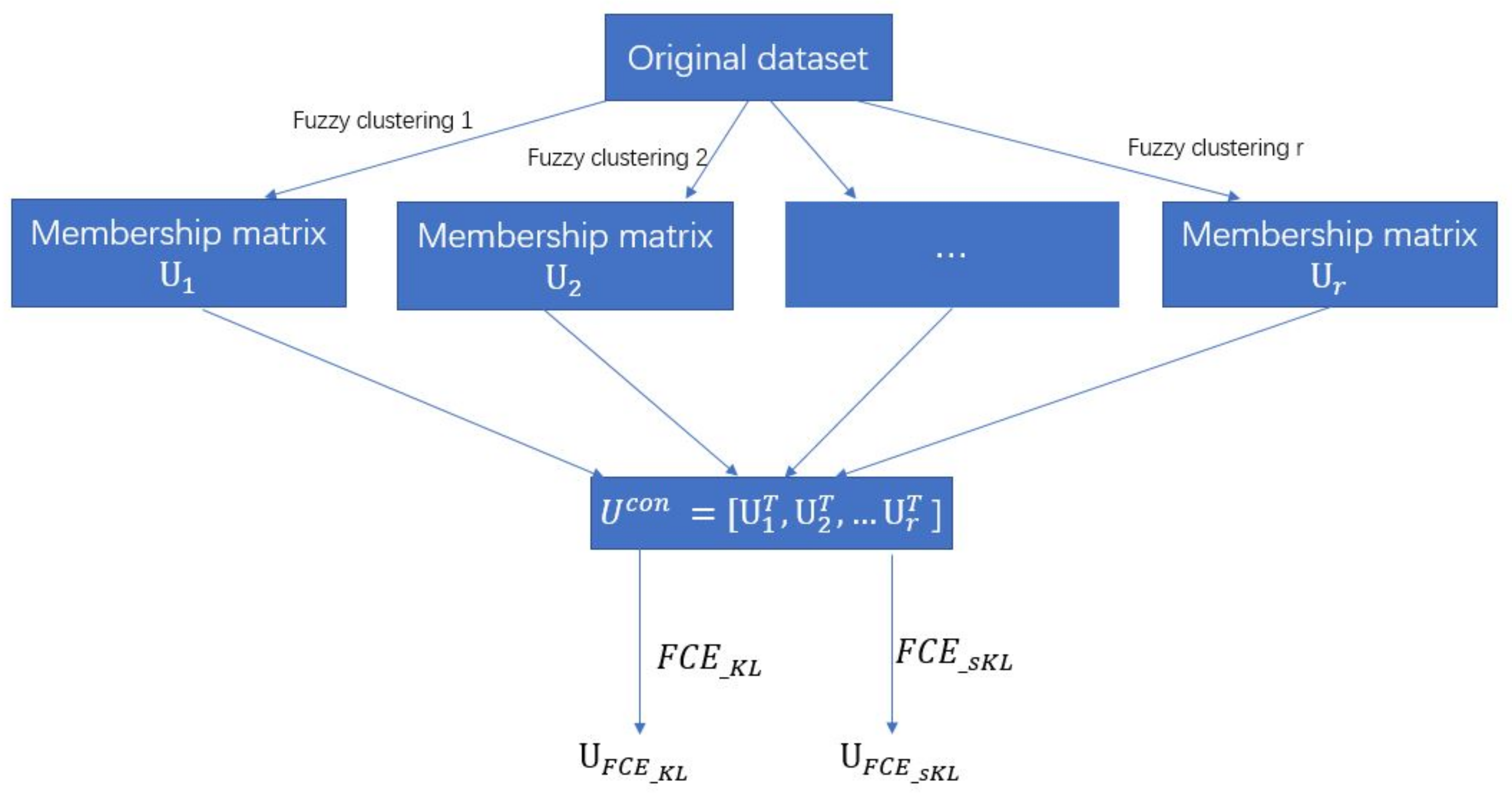
3.1. Formulation of the Fuzzy Cluster Ensemble Problem
3.2. Fuzzy Cluster Ensemble Based on KL Divergence ()
3.3. Spatial Information-Based
| Algorithm 1: |
| Input: Normalized partitions , values of the fuzzification coefficient m, maximum iteration number and a small enough error Output: The consensus clustering;
|
4. Experiment Results
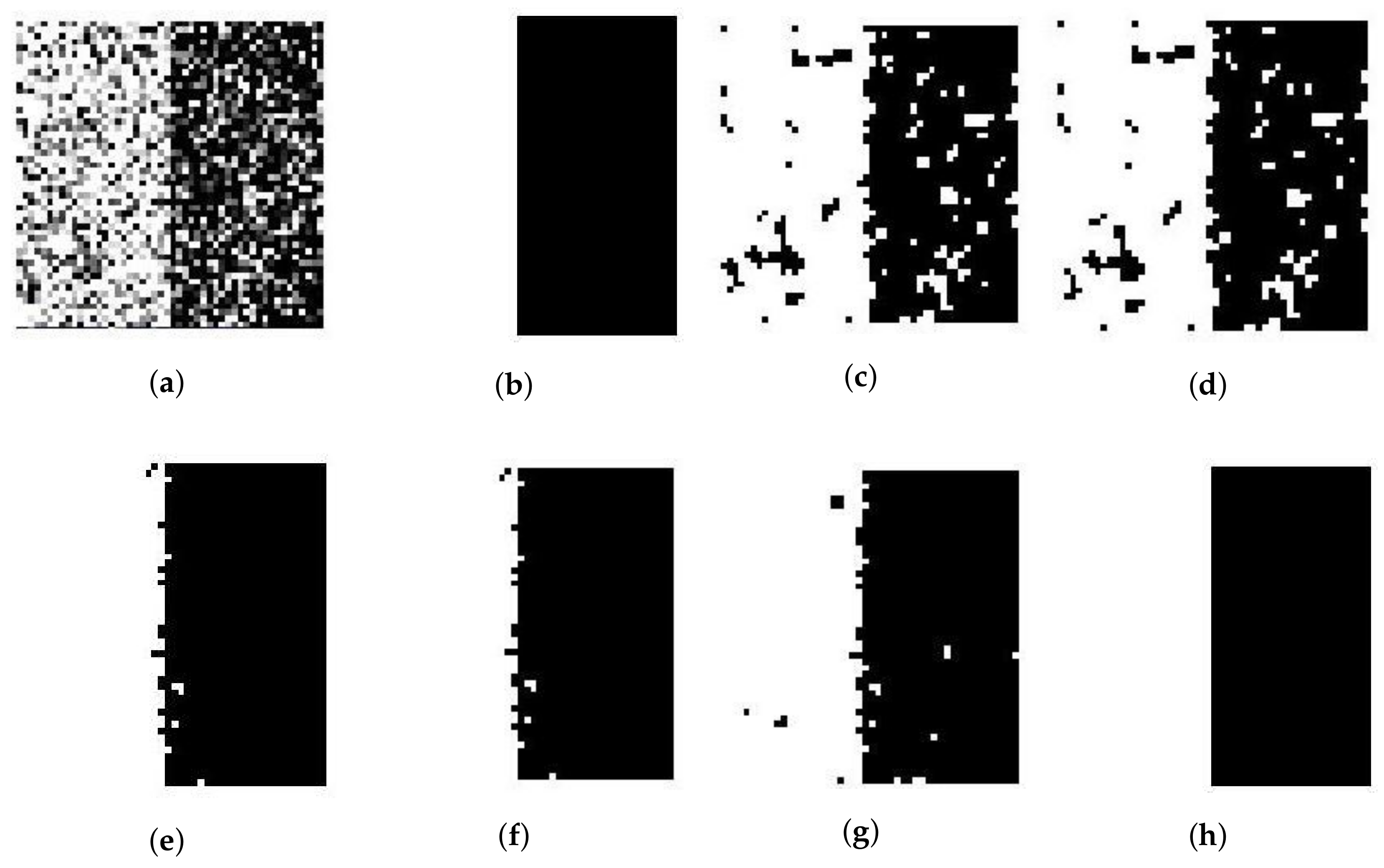
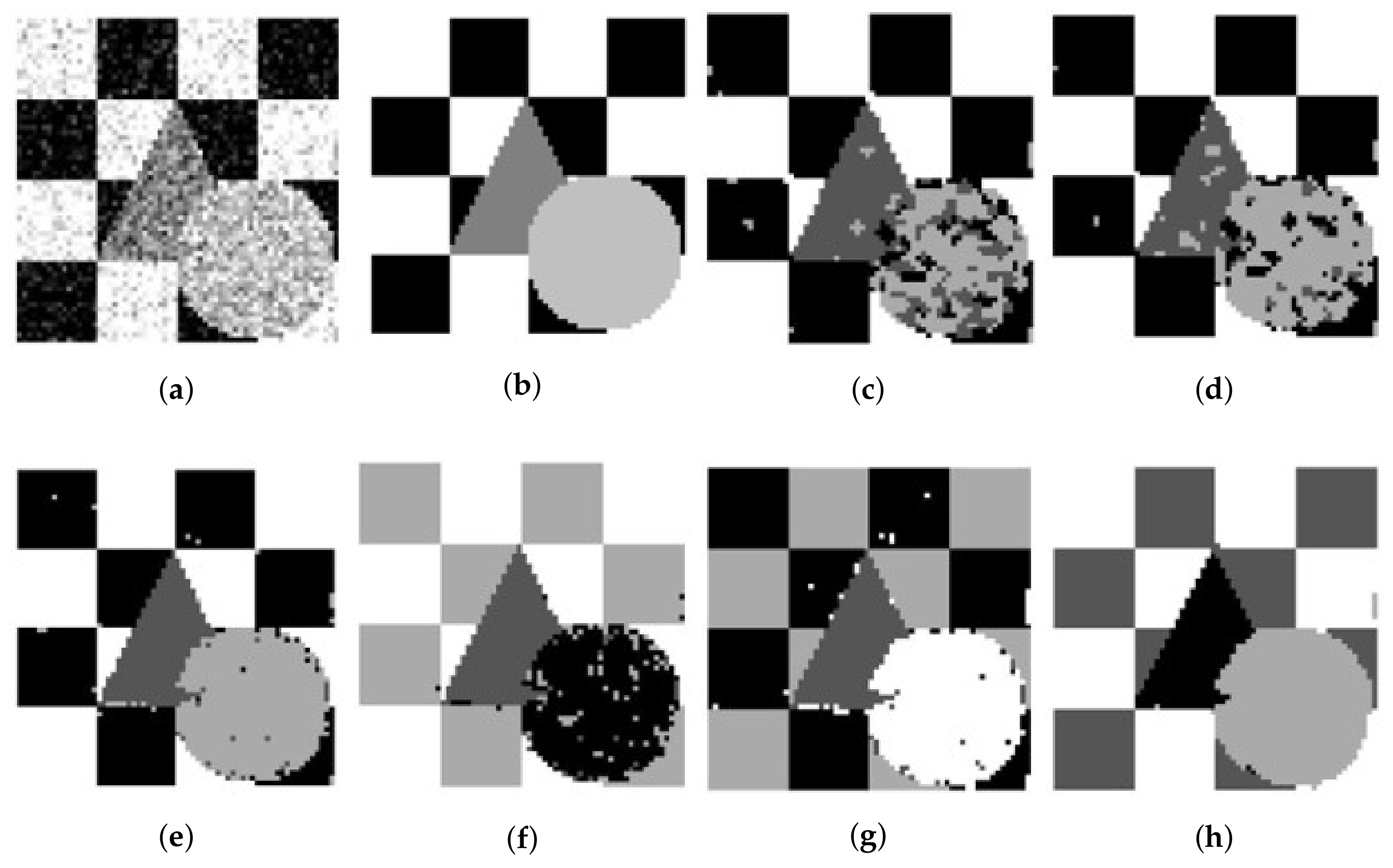
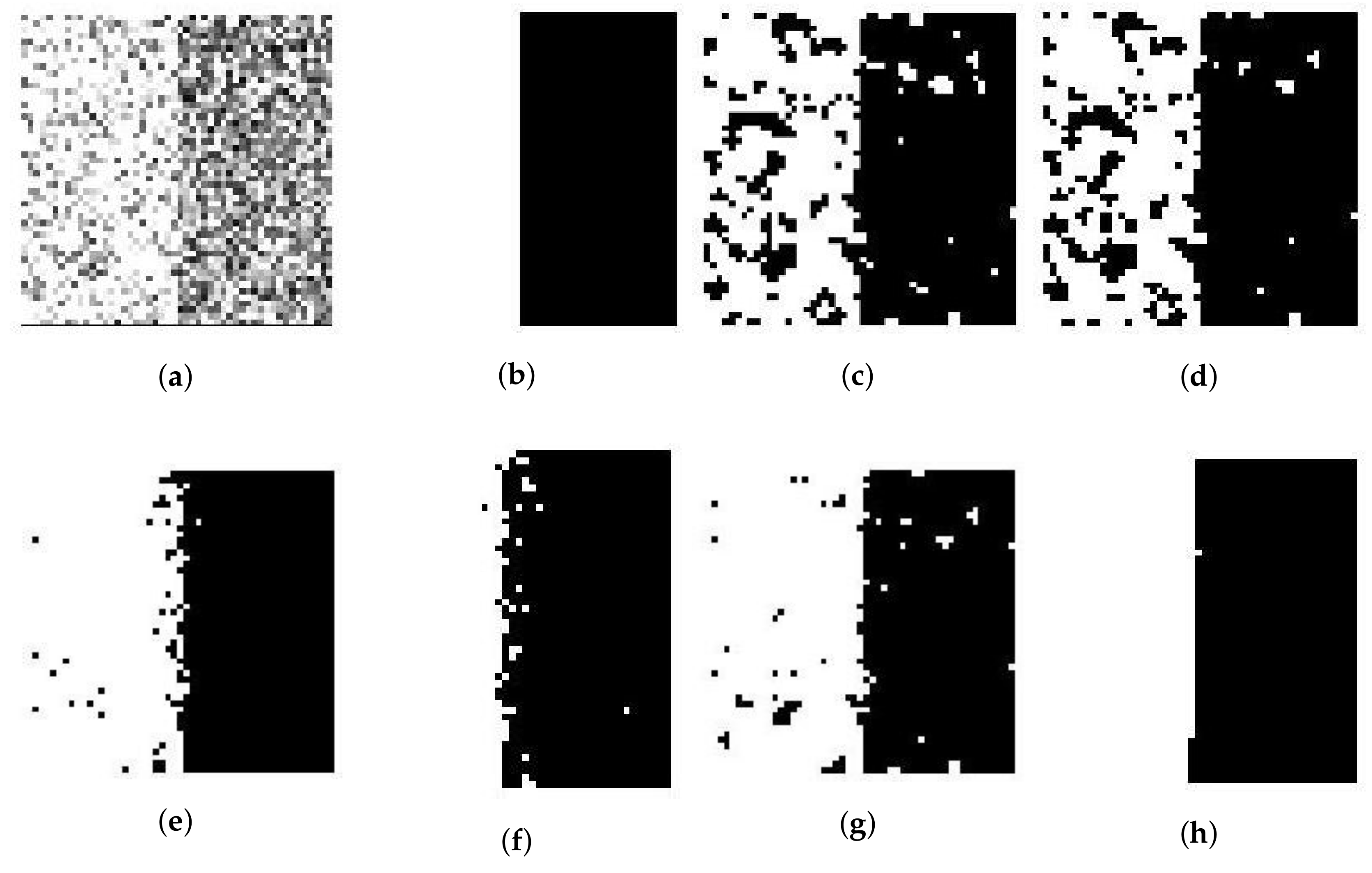
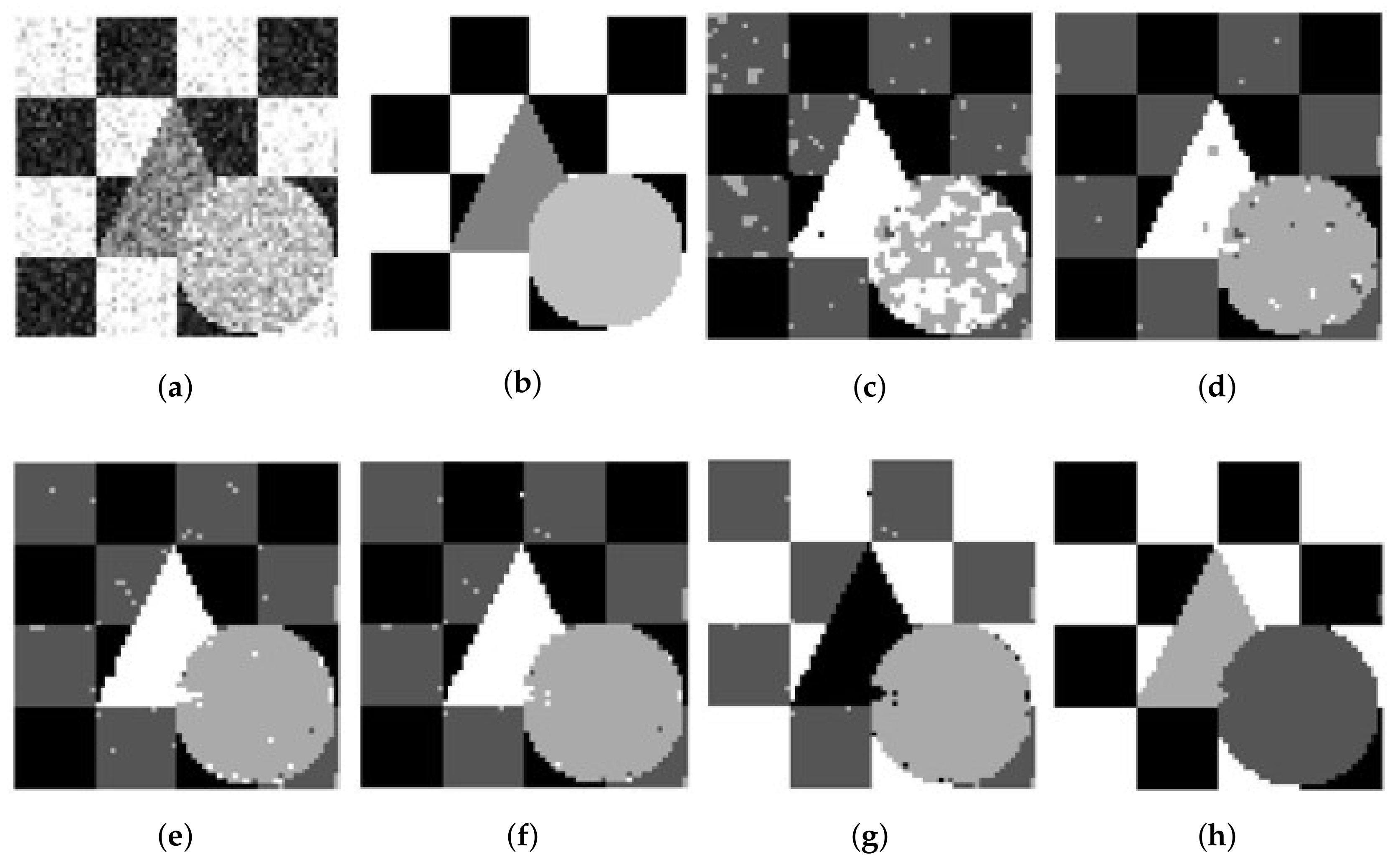
4.1. Synthetic Images
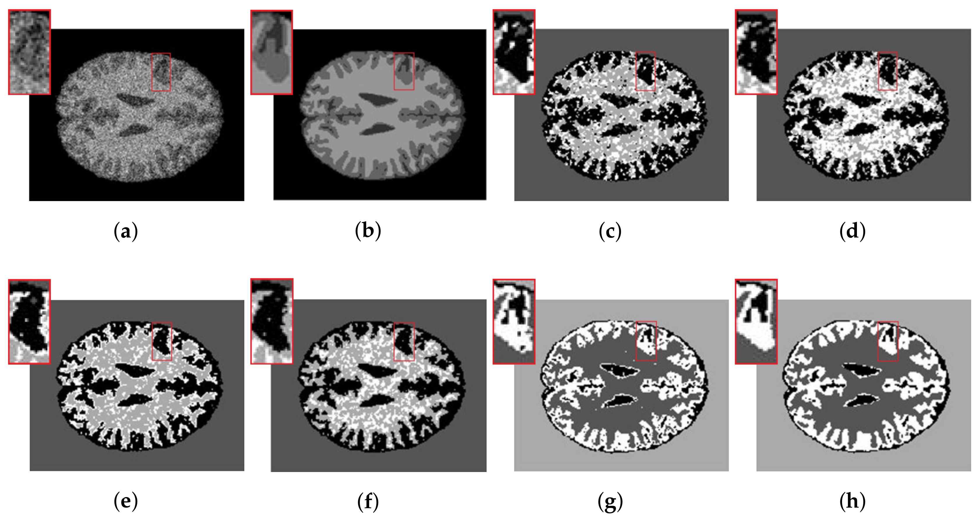
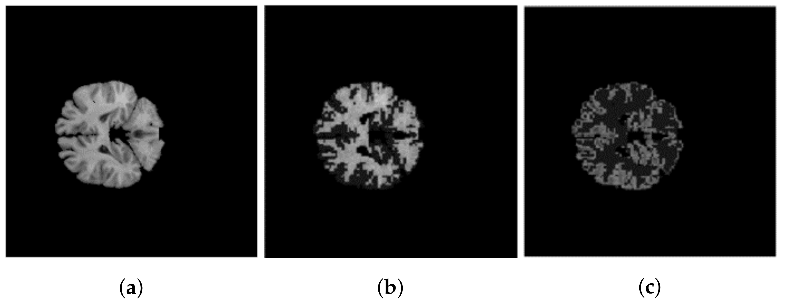
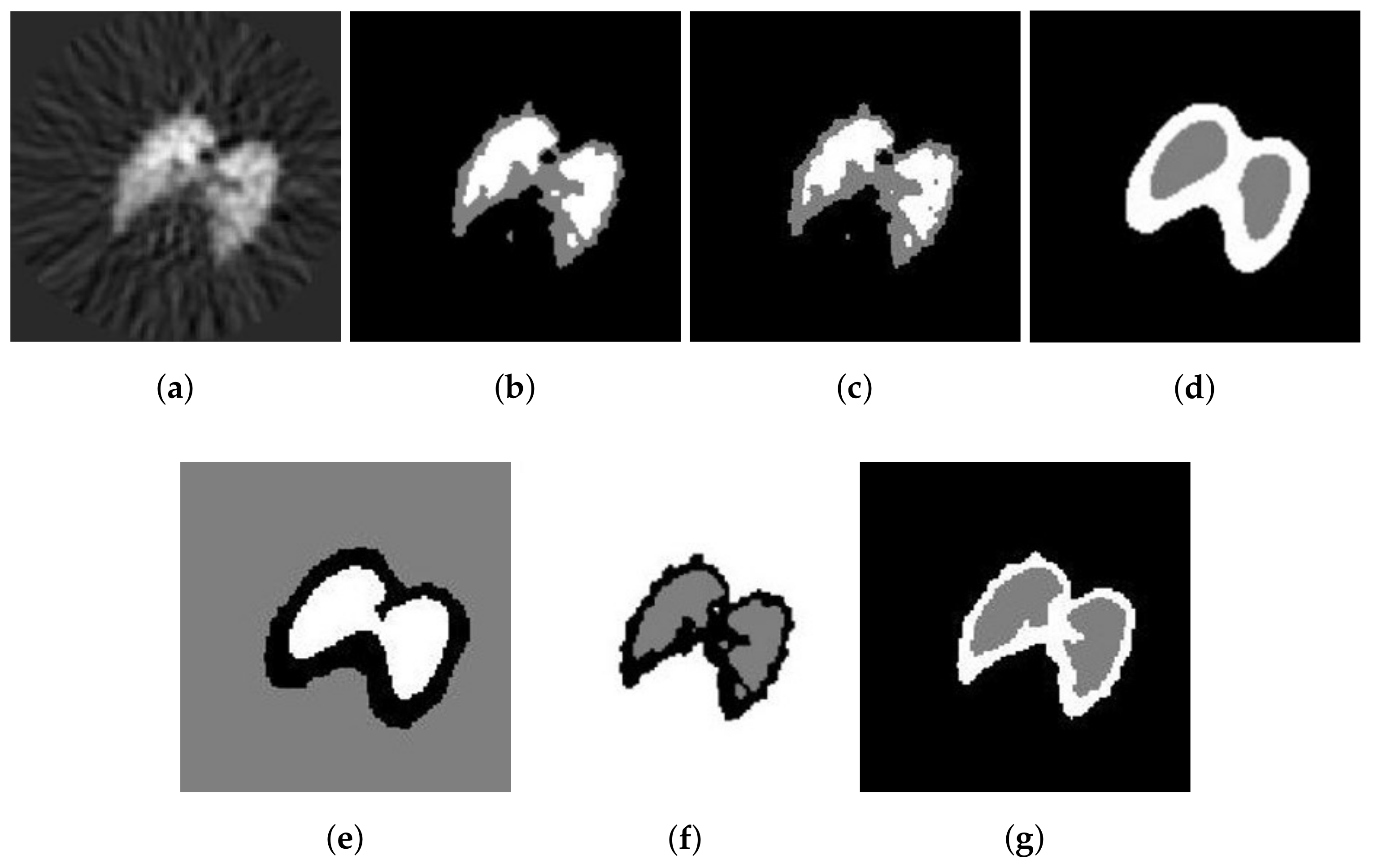
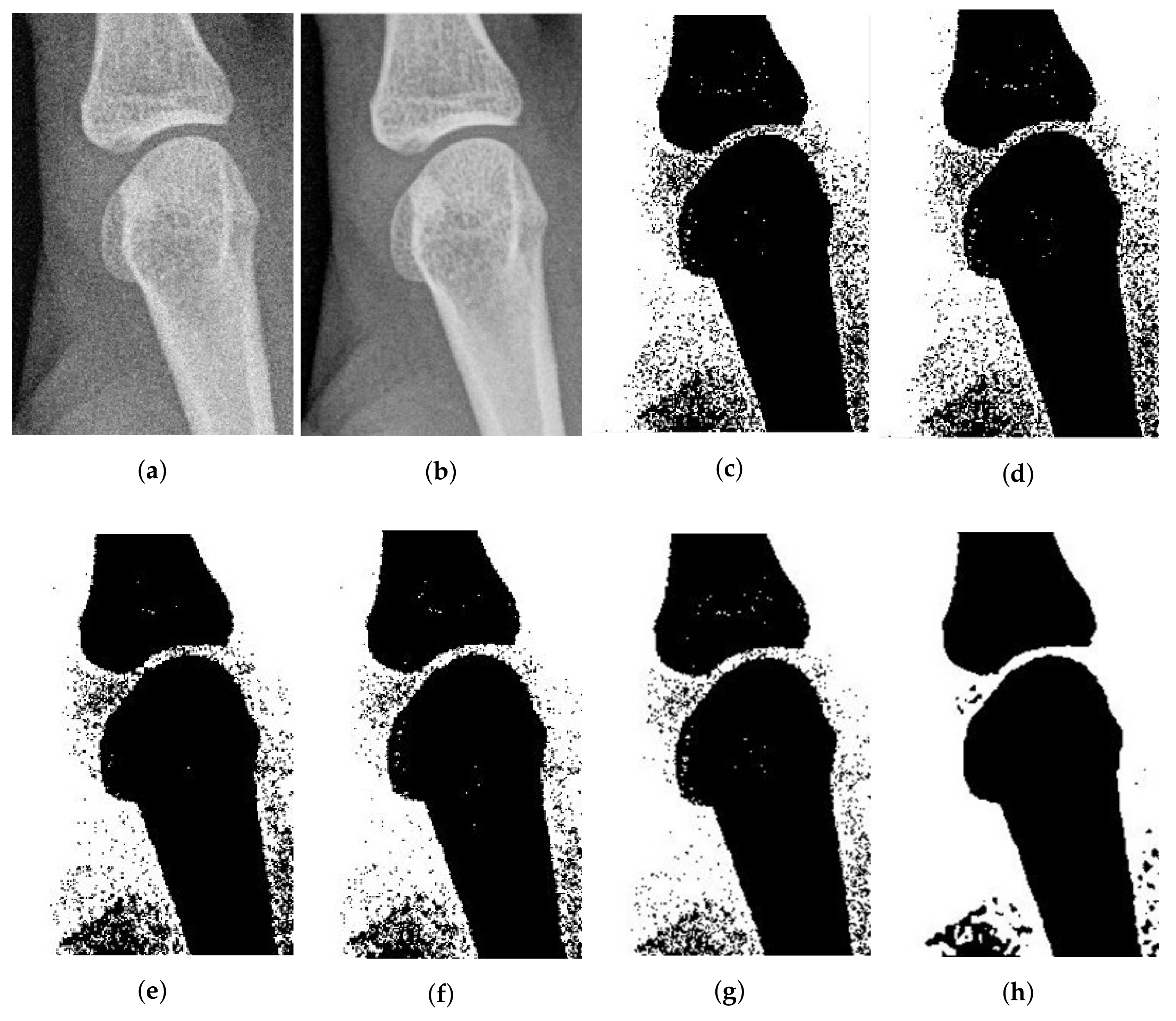
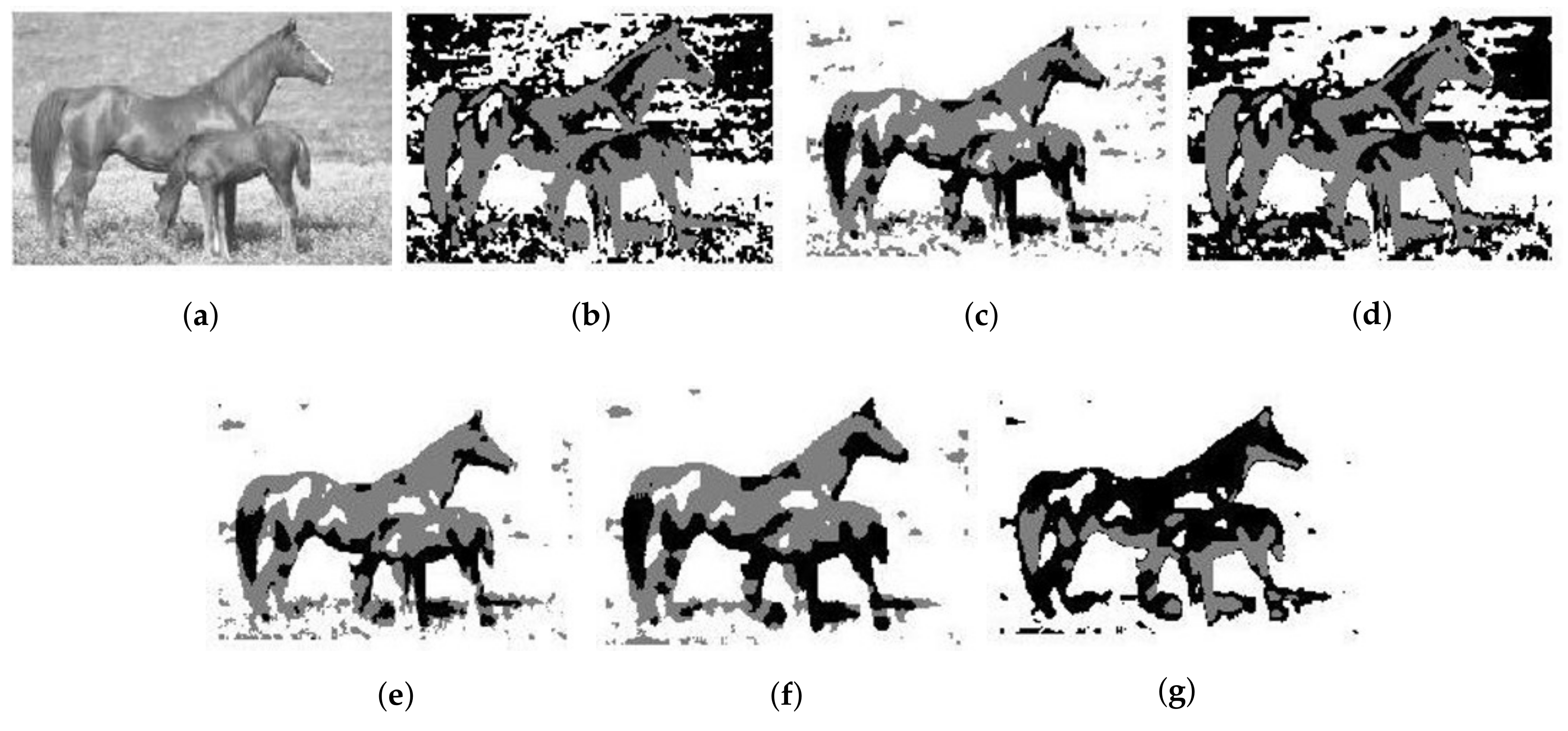
4.2. Real Images
5. Discussion
6. Conclusions
Acknowledgments
Author Contributions
Conflicts of Interest
Abbreviations
| Fuzzy cluster ensemble method based on KL divergence | |
| Spatial |
References
- Arslan, S.; Ersahin, T.; Cetin-Atalay, R.; Gunduz-Demir, C. Attributed relational graphs for cell nucleus segmentation in fluorescence microscopy images. IEEE Trans. Med. Imaging 2013, 32, 1121–1131. [Google Scholar] [CrossRef] [PubMed]
- Chen, S.; Zhang, D. Robust image segmentation using FCM with spatial constraints based on new kernel-induced distance measure. IEEE Trans. Syst. Man Cybern. Part B 2004, 34, 1907–1916. [Google Scholar] [CrossRef]
- Caponetti, L.; Castellano, G.; Corsini, V. MR Brain Image Segmentation: A Framework to Compare Different Clustering Techniques. Information 2017, 8, 138. [Google Scholar] [CrossRef]
- Shen, P.; Li, C. Local feature extraction and information bottleneck-based segmentation of brain magnetic resonance (mr) images. Entropy 2013, 15, 3205–3218. [Google Scholar] [CrossRef]
- Bogoslavskyi, I.; Stachniss, C. Fast range image-based segmentation of sparse 3D laser scans for online operation. In Proceedings of the 2016 IEEE/RSJ International Conference on Intelligent Robots and Systems (IROS), Daejeon, South Korea, 9–14 October 2016; pp. 163–169. [Google Scholar]
- Huang, D.; Lai, J.H.; Wang, C.D.; Yuen, P.C. Ensembling over-segmentations: From weak evidence to strong segmentation. Neurocomputing 2016, 207, 416–427. [Google Scholar] [CrossRef]
- Pont-Tuset, J.; Arbelaez, P.; Barron, J.T.; Marques, F.; Malik, J. Multiscale combinatorial grouping for image segmentation and object proposal generation. IEEE Trans. Pattern Anal. Mach. Intell. 2017, 39, 128–140. [Google Scholar] [CrossRef] [PubMed]
- Guo, L.; Chen, L.; Wu, Y.; Chen, C.P. Image Guided Fuzzy C-Means for Image Segmentation. In Proceedings of the 2016 IEEE International Conference on Systems, Man, and Cybernetics (SMC), Budapest, Hungary, 9–12 October 2016; pp. 1–10. [Google Scholar]
- Chuang, K.S.; Tzeng, H.L.; Chen, S.; Wu, J.; Chen, T.J. Fuzzy c-means clustering with spatial information for image segmentation. Comput. Med. Imaging Graph. 2006, 30, 9–15. [Google Scholar] [CrossRef] [PubMed]
- Liew, A.W.C.; Yan, H. An adaptive spatial fuzzy clustering algorithm for 3-D MR image segmentation. IEEE Trans. Med. Imaging 2003, 22, 1063–1075. [Google Scholar] [CrossRef] [PubMed]
- Zang, W.; Zhang, W.; Zhang, W.; Liu, X. A kernel-based intuitionistic fuzzy C-means clustering using a DNA genetic algorithm for magnetic resonance image segmentation. Entropy 2017, 19, 578. [Google Scholar] [CrossRef]
- Bezdek, J.C.; Ehrlich, R.; Full, W. FCM: The fuzzy c-means clustering algorithm. Comput. Geosci. 1984, 10, 191–203. [Google Scholar] [CrossRef]
- Mitra, S.; Pedrycz, W.; Barman, B. Shadowed c-means: Integrating fuzzy and rough clustering. Pattern Recognit. 2010, 43, 1282–1291. [Google Scholar] [CrossRef]
- Chen, L.; Chen, C.P.; Lu, M. A multiple-kernel fuzzy c-means algorithm for image segmentation. IEEE Trans. Syst. Man Cybern. Part B 2011, 41, 1263–1274. [Google Scholar] [CrossRef] [PubMed]
- Topchy, A.; Jain, A.K.; Punch, W. Clustering ensembles: Models of consensus and weak partitions. IEEE Trans. Pattern Anal. Mach. Intell. 2005, 27, 1866–1881. [Google Scholar] [CrossRef] [PubMed]
- Zou, J.; Chen, L.; Chen, C.P. Ensemble fuzzy c-means clustering algorithms based on KL divergence for medical image segmentation. In Proceedings of the 2013 IEEE International Conference on Bioinformatics and Biomedicine (BIBM), Shanghai, China, 18–21 December 2013; pp. 291–296. [Google Scholar]
- Rathore, P.; Bezdek, J.C.; Erfani, S.M.; Rajasegarar, S.; Palaniswami, M. Ensemble Fuzzy Clustering using Cumulative Aggregation on Random Projections. IEEE Trans. Fuzzy Syst. 2017, PP, 1. [Google Scholar] [CrossRef]
- Fred, A.L.; Jain, A.K. Combining multiple clusterings using evidence accumulation. IEEE Trans. Pattern Anal. Mach. Intell. 2005, 27, 835–850. [Google Scholar] [CrossRef] [PubMed]
- Iam-On, N.; Boongeon, T.; Garrett, S.; Price, C. A link-based cluster ensemble approach for categorical data clustering. IEEE Trans. Knowl. Data Eng. 2012, 24, 413–425. [Google Scholar] [CrossRef]
- Fred, A.; Lourenço, A. Cluster ensemble methods: from single clusterings to combined solutions. In Supervised and Unsupervised Ensemble Methods and Their Applications; Springer: Berlin/Heidelberg, Germany, 2008; pp. 3–30. [Google Scholar]
- Wan, X.; Lin, H.; Li, H.; Liu, G.; An, M. Ensemble clustering via Fuzzy c-Means. In Proceedings of the 2017 International Conference on Service Systems and Service Management (ICSSSM), Dalian, China, 16–18 June 2017; pp. 1–6. [Google Scholar]
- Sengottaian, S.; Natesan, S.; Mathivanan, S. Weighted Delta Factor Cluster Ensemble Algorithm for Categorical Data Clustering in Data Mining. Int. Arab J. Inf. Technol. (IAJIT) 2017, 14, 275–284. [Google Scholar]
- Wu, J.; Wu, Z.; Cao, J.; Liu, H.; Chen, G.; Zhang, Y. Fuzzy Consensus Clustering With Applications on Big Data. IEEE Trans. Fuzzy Syst. 2017, 25, 1430–1445. [Google Scholar] [CrossRef]
- Punera, K.; Ghosh, J. Soft cluster ensembles. In Advances in Fuzzy Clustering and Its Applications; Wiley: Hoboken, NJ, USA, 2007; pp. 69–90. [Google Scholar]
- Zou, J.; Chen, L.; Chen, C.P. Shadowed C-means for image segmentation using local and nonlocal spatial information. In Proceedings of the 2013 IEEE International Conference on Systems, Man, and Cybernetics (SMC), Manchester, UK, 13–16 October 2013; pp. 3933–3938. [Google Scholar]
- Yi, J.; Yang, T.; Jin, R.; Jain, A.K.; Mahdavi, M. Robust ensemble clustering by matrix completion. In Proceedings of the 2012 IEEE 12th International Conference on Data Mining (ICDM), Brussels, Belgium, 10–13 December 2012; pp. 1176–1181. [Google Scholar]
- Li, T.; Chen, Y. Fuzzy clustering ensemble algorithm for partitioning categorical data. In Proceedings of the BIFE’09 International Conference on Business Intelligence and Financial Engineering, Beijing, China, 24–26 July 2009; pp. 170–174. [Google Scholar]
- Strehl, A.; Ghosh, J. Cluster ensembles—A knowledge reuse framework for combining multiple partitions. J. Mach. Learn. Res. 2002, 3, 583–617. [Google Scholar]
- Yu, Z.; Li, L.; Gao, Y.; You, J.; Liu, J.; Wong, H.S.; Han, G. Hybrid clustering solution selection strategy. Pattern Recognit. 2014, 47, 3362–3375. [Google Scholar] [CrossRef]
- Cocosco, C.A.; Kollokian, V.; Kwan, R.K.S.; Pike, G.B.; Evans, A.C. Brainweb: Online interface to a 3D MRI simulated brain database. NeuroImage 1996, 5, 425. [Google Scholar]
- NeuroInformatics Tools and Resources Collaboratory. Available online: http://www.cma.mgh.harvard.edu/ibsr/ (accessed on 3 April 2018).
- Kennedy, D.N.; Filipek, P.A.; Caviness, V.S. Anatomic segmentation and volumetric calculations in nuclear magnetic resonance imaging. IEEE Trans. Med. Imaging 1989, 8, 1–7. [Google Scholar] [CrossRef] [PubMed]
- Schwämmle, V.; Jensen, O.N. A simple and fast method to determine the parameters for fuzzy c–means cluster analysis. Bioinformatics 2010, 26, 2841–2848. [Google Scholar] [CrossRef] [PubMed]
- Wu, K.L. Analysis of parameter selections for fuzzy c-means. Pattern Recognit. 2012, 45, 407–415. [Google Scholar] [CrossRef]
- Tibshirani, R.; Walther, G.; Hastie, T. Estimating the number of clusters in a dataset via the gap statistic. J. R. Stat. Soc. Ser. B Stat. Methodol. 2001, 63, 411–423. [Google Scholar] [CrossRef]
- Milligan, G.W.; Cooper, M.C. An examination of procedures for determining the number of clusters in a dataset. Psychometrika 1985, 50, 159–179. [Google Scholar] [CrossRef]


| 0.7 | 0.2 | 0.1 | 0.1 | 0.7 | 0.2 | 0.7 | 0.2 | 0.1 | 0.1 | 0.7 | 0.2 | 0.35 | 0.10 | 0.05 | 0.05 | 0.35 | 0.10 | ||||
| 0.9 | 0.1 | 0.0 | 0.0 | 0.8 | 0.2 | 0.9 | 0.1 | 0.0 | 0.0 | 0.8 | 0.2 | 0.45 | 0.05 | 0.00 | 0.00 | 0.40 | 0.10 | ||||
| 0.2 | 0.6 | 0.2 | 0.1 | 0.1 | 0.8 | 0.2 | 0.6 | 0.2 | 0.1 | 0.1 | 0.8 | 0.10 | 0.30 | 0.10 | 0.05 | 0.05 | 0.40 | ||||
| 0.1 | 0.9 | 0.0 | 0.2 | 0.1 | 0.7 | 0.1 | 0.9 | 0.0 | 0.2 | 0.1 | 0.7 | 0.05 | 0.45 | 0.00 | 0.10 | 0.05 | 0.35 | ||||
| 0.1 | 0.2 | 0.7 | 0.6 | 0.2 | 0.2 | 0.1 | 0.2 | 0.7 | 0.6 | 0.2 | 0.2 | 0.05 | 0.10 | 0.35 | 0.30 | 0.10 | 0.10 | ||||
| SA | SFCM | SSCM | NLSFCM | NLSSCM | ||
|---|---|---|---|---|---|---|
| 1% Gaussian | ||||||
| 3% Gaussian | ||||||
| 5% Gaussian | ||||||
| 10% Gaussian | 0.9992 | 0.9992 | 0.9996 | 0.9996 | 0.9996 | |
| 15% Gaussian | 0.9984 | 0.9980 | 0.9992 | 0.9992 | 0.9992 | |
| 20% Gaussian | 0.9928 | 0.9932 | 0.9988 | 0.9988 | 0.9988 | |
| 30% Gaussian | 0.9732 | 0.9760 | 0.9976 | 0.9976 | 0.9956 | |
| 50% Gaussian | 0.9100 | 0.9148 | 0.9916 | 0.9916 | 0.9808 | |
| 1% Rician | ||||||
| 3% Rician | ||||||
| 5% Rician | ||||||
| 10% Rician | ||||||
| 15% Rician | ||||||
| 20% Rician | ||||||
| 30% Rician | 0.9956 | 0.9960 | 0.9988 | 0.9988 | 0.9988 | |
| 50% Rician | 0.8640 | 0.8664 | 0.9744 | 0.9828 | 0.9678 |
| SA | SFCM | SSCM | NLSFCM | NLSSCM | ||
|---|---|---|---|---|---|---|
| 10% Gaussian | 0.9817 | 0.9878 | 0.9946 | 0.9951 | 0.9966 | |
| 12% Gaussian | 0.9563 | 0.9712 | 0.9893 | 0.9817 | 0.9922 | |
| 15% Gaussian | 0.8979 | 0.9348 | 0.9800 | 0.9670 | 0.9797 | |
| 18% Gaussian | 0.8420 | 0.8896 | 0.9624 | 0.9138 | 0.9631 | |
| 20% Gaussian | 0.8218 | 0.8457 | 0.9290 | 0.8937 | 0.9468 | |
| 25% Gaussian | 0.7729 | 0.7773 | 0.7847 | 0.7813 | 0.9026 | |
| 30% Gaussian | 0.6860 | 0.7446 | 0.7341 | 0.7539 | 0.7239 | |
| 10% Rician | 0.9839 | 0.9917 | 0.9919 | 0.9934 | 0.9954 | |
| 12% Rician | 0.8782 | 0.9768 | 0.9817 | 0.9888 | 0.9897 | |
| 15% Rician | 0.7578 | 0.7136 | 0.9209 | 0.9670 | 0.9758 | |
| 18% Rician | 0.7114 | 0.7112 | 0.7886 | 0.9526 | 0.9570 | |
| 20% Rician | 0.6799 | 0.7085 | 0.7598 | 0.8413 | 0.9377 | |
| 25% Rician | 0.6650 | 0.6775 | 0.7681 | 0.7531 | 0.8472 | |
| 30% Rician | 0.6287 | 0.6406 | 0.6914 | 0.6818 | 0.7832 |
| SA | SFCM | SSCM | NLSFCM | NLSSCM | ||
|---|---|---|---|---|---|---|
| 25% Rician | 0.8523 | 0.8125 | 0.8438 | 0.9543 | 0.9692 | |
| 27% Rician | 0.8473 | 0.8117 | 0.8411 | 0.8504 | 0.9669 | |
| 30% Rician | 0.8405 | 0.8070 | 0.8391 | 0.8411 | 0.9605 | |
| 32% Rician | 0.8373 | 0.8026 | 0.8393 | 0.8339 | 0.9559 | |
| 35% Rician | 0.8321 | 0.7966 | 0.8390 | 0.8317 | 0.9485 | |
| 40% Rician | 0.8160 | 0.7903 | 0.8395 | 0.8249 | 0.9361 | |
| 50% Rician | 0.7804 | 0.7784 | 0.8610 | 0.7911 | 0.9074 |
| 12% Rician Noise | SFCM | SSCM | NLSFCM | NLSSCM | ||
|---|---|---|---|---|---|---|
| SA | 0.7293 | 0.7400 | 0.7181 | 0.7163 | 0.7247 | |
| 0.7463 | 0.7530 | 0.7297 | 0.7247 | 0.7381 | ||
| 0.7099 | 0.7256 | 0.7055 | 0.7073 | 0.7098 |
| 15% Rician Noise | SFCM | SSCM | NLSFCM | NLSSCM | ||
|---|---|---|---|---|---|---|
| SA | 0.7079 | 0.7237 | 0.7023 | 0.7093 | 0.7098 | |
| 0.7281 | 0.7431 | 0.7248 | 0.7421 | 0.7369 | ||
| 0.6844 | 0.7012 | 0.6758 | 0.6670 | 0.6763 |
| 18% Rician Noise | SFCM | SSCM | NLSFCM | NLSSCM | ||
|---|---|---|---|---|---|---|
| SA | 0.6744 | 0.7014 | 0.6879 | 0.7028 | 0.6953 | |
| 0.7031 | 0.7268 | 0.7205 | 0.7584 | 0.7338 | ||
| 0.6395 | 0.6708 | 0.6467 | 0.6139 | 0.6438 |
© 2018 by the authors. Licensee MDPI, Basel, Switzerland. This article is an open access article distributed under the terms and conditions of the Creative Commons Attribution (CC BY) license (http://creativecommons.org/licenses/by/4.0/).
Share and Cite
Wei, H.; Chen, L.; Guo, L. KL Divergence-Based Fuzzy Cluster Ensemble for Image Segmentation. Entropy 2018, 20, 273. https://doi.org/10.3390/e20040273
Wei H, Chen L, Guo L. KL Divergence-Based Fuzzy Cluster Ensemble for Image Segmentation. Entropy. 2018; 20(4):273. https://doi.org/10.3390/e20040273
Chicago/Turabian StyleWei, Huiqin, Long Chen, and Li Guo. 2018. "KL Divergence-Based Fuzzy Cluster Ensemble for Image Segmentation" Entropy 20, no. 4: 273. https://doi.org/10.3390/e20040273
APA StyleWei, H., Chen, L., & Guo, L. (2018). KL Divergence-Based Fuzzy Cluster Ensemble for Image Segmentation. Entropy, 20(4), 273. https://doi.org/10.3390/e20040273