Abstract
Establishing policies for controlling water pollution through discharge permits creates the basis for emission permit trading. Allocating wastewater discharge permits is a prerequisite to initiating the market. Past research has focused on designing schemes to allocate discharge permits efficiently, but these schemes have ignored differences among regions in terms of emission history. This is unfortunate, as fairness may dictate that areas that have been allowed to pollute in the past will receive fewer permits in the future. Furthermore, the spatial scales of previously proposed schemes are not practical. In this article, we proposed an information entropy improved proportional allocation method, which considers differences in GDP, population, water resources, and emission history at province spatial resolution as a new way to allocate waste water emission permits. The allocation of chemical oxygen demand (COD) among 30 provinces in China is used to illustrate the proposed discharge permit distribution mechanism. In addition, we compared the pollution distribution permits obtained from the proposed allocation scheme with allocation techniques that do not consider historical pollution and with the already established country plan. Our results showed that taking into account emission history as a factor when allocating wastewater discharge permits results in a fair distribution of economic benefits.
1. Introduction
Total pollution load regulation controls total wastewater emission and can be used to control environmental quality [1]. Such policies have been applied in developed countries such as United States of America and Japan [2,3,4,5]. Developing countries like China are also experimenting with similar regulation. These schemes make the discharge permits a scarce resource. As a result, different regions compete for allocation permits. Each region desires to gain higher wastewater emission permits, since emission permits directly influences economic development [6,7]. Therefore, the uneven distribution of wastewater discharge permits leads to the uneven distribution of economic benefits [8,9,10,11].
Careful design of wastewater policy is necessary for these policies to be effective [12,13]. One factor that needs to be considered to achieve this goal is to align the spatial resolution of the allocation policy and the political management zones. Most of the previous studies in China were done at the river basin spatial scale and mainly focused on quantifying the impact of the upstream activities on the downstream allocation [14,15,16,17]. Studies at practical spatial management scales are very important for the implementation of proposed emission allocation schemes. This is the reason why our study is conducted at the province scale.
In addition to the spatial scale, any allocation framework should take in to account the historical emission trend of the provinces in order to ensure fair distribution of discharge permits [18,19]. Considering historical responsibility while allocating permits has been extensively used in greenhouse-gas emission quota allocation [20,21]. Wastewater discharge permits are often allocated through auctioning or grandfathering. Auctions aim to create economically efficient distributions and have been widely used in carbon markets [22,23]. However, due to the huge potential cost of non-cooperation among stakeholders, the distribution mechanism of auctioning has been increasingly questioned [24]. One of the big challenges in wastewater emission permit allocation is fitting historical responsibility into the existing allocation frameworks. Grandfathering takes historical responsibility into account but is not efficient.
Aiming to mitigate the above drawbacks, we proposed a new wastewater permit distribution mechanism that takes into account fairness by considering emission history at the provincial scale. As one of the main wastewater discharge pollutants, the allocation of chemical oxygen demand (COD) emission permits among the 30 provinces of China is used to illustrate the proposed mechanism and compare results with the existing country plan as well as with the results from methods proposed by recent studies.
2. Methods
2.1. Study Area
The objective of this research is to distribute China’s 2020 wastewater COD discharge permits among 30 provinces (As shown in Figure 1, Tibet is not included because it has little wastewater discharge and the historical data is also unavailable) with 2015 as the target year for the allocation. Since 1996, the Chinese government has developed a total pollution load control policy and allocated wastewater discharge permits to each administrative province every five years based on current pollution load [7]. However, the central government’s uniform pollution permit distribution scheme does not consider each province’s social, economic, and environmental differences. Hence, the allocation may not respect the principle of equity and could cause big dissatisfaction among the provinces [6]. With increasing water pollution in China [25], wastewater discharge allocation policy that is fair to all provinces is very important for sustainable development in China.
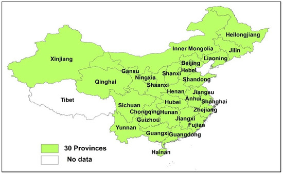
Figure 1.
The 30 provinces of mainland China.
China’s water resource management structure is based on political management structure rather than on geographic location [14]. Usually, the first step is for the central government’s Environmental Protection Bureau to decide the total wastewater discharge permit for each province [6,7]. This step is very crucial and challenging because each province is autonomous and competes for more emission discharge permits since a higher discharge permit can be translated directly to more economic benefits. As a result, each province acts as a utility-maximizing agent.
Mainland China’s 30 provinces differ greatly in their economic growth, social features, and environment [26]. Previously, to promote economic prosperity, the Chinese government allowed some provinces to pollute more without bearing the cost of pollution [27]. Currently, the Chinese government is attempting an environmentally friendly development path and is internalizing pollution cost within development efforts. Applying such policy equally to all the 30 provinces might not be fair because these provinces have different socio-economic and environmental makeups but most importantly their emission history is highly asymmetric.
2.2. Data
The period for the study is from 2000 to 2020. This period covers two decades of major economic growth for China and is a period with well-documented data. The gross domestic product (GDP) and population data of each province for the period from 2000–2015 are obtained from China Statistical Yearbook [28]. Each province’s chemical oxygen demand (COD) emission data from for the study period is obtained from China Environment Yearbook [29]. The water capital of each province for the time period under consideration were extracted from China Water Resources Bulletin [30]. To eliminate the impact of inflation, the GDP was deflated by using 2000 as the base year.
2.3. Historical Pollution and Emissions Discrepancies
Before distributing the total wastewater discharge permits, we need to understand the differences among provinces in terms of pollution history to ensure equity. In this part, we choose GDP as one factor, to analyze the historical discrepancies among provinces.
Assume is the number of provinces in China and m represents the mth province.
For the period from year x to y, is the mth province’s GDP proportion and can be determined as follows:
For the period x to y, is the mth province’s COD proportion and can be computed as follows:
Then, province deviation coefficient can be calculated as:
If is greater than one, this indicates that the proportion of historical COD emission in this province is greater than the proportion of GDP. This means the province’s GDP increase is associated with decreasing quality of the aquatic environment as the result of increased COD emissions. Using the same procedure, we can obtain and . If the values of deviation coefficients for these parameters are greater than 1, then COD emission increases proportionally with GDP, population, and water capital. These three dimensions provide insight on whether each province’s development path needs to change. For example, when a province’s , it indicates that the environment is disproportionately damaged and the development path should change to a more environmentally friendly economic development model.
2.4. Entropy-Improved Proportional Method for Wastewater Discharge Permit Allocation
The entropy method is an objective way of weighing and measuring the disorder of a system [31,32]. By calculating entropy, we determine the weight that reflects the different pollution level among provinces [33].
The disadvantage of this method is that it does not consider the differences among the provinces. Using the entropy method avoids this shortcoming. Hence the wastewater emission permit allocation satisfies the principles of equity, efficiency, and sustainability. The detailed procedure is as follows.
Suppose the status of province i’s emission is qi, a is the GDP index, population, and water capital.
is the value of province from index a.
The first step is the standardization of :
For the positive index: .
For the negative index: .
Here, we considered population and water capital as indicators. There are some principles for reducing wastewater discharge permits. First, those with higher GDP should reduce more because they have greater ability and resources to reduce COD emission while maintaining their economic development. Second, provinces with higher population should cut less since every person has an equal right to COD emission. Third, those with more water capital should cut down less because they can assimilate more COD. Thus, we can see that GDP is a positive index, while population and water capital are negative indices.
The weight of province from index a can be determined as follows.
The information entropy () of province from can index a be computed as follows.
The weight of the index a is calculated using the entropy method [34,35].
The method we suggest here is the information entropy improved proportional allocation method. The equal allocation method reduces each province’s emission proportionally. Information entropy improved means that, according to the principle of fairness, provinces adjust the equal-proportional allocation method. The greater the differences among provinces, the greater the disparities in terms of emission reductions. On the contrary, when regional differences are negligible, the emission reductions of the provinces are more similar.
Assuming the total target reduction rate is b, qi is the province ith COD emission for the base year (2015), the total COD emission of provinces () participating in waste water discharge permit allocation for the base year (the year of 2015) is .
Then, province i’s reduction rate will be:
where, is the average reduction rate for each province, is the relative difference of province i.
is determined by GDP, population and water capital indices. Firstly, each province’s difference score is calculated as,
Then, is computed as follows;
The average reduction the rate for province i will be:
Finally, the emission reduction and amount variables are determined as follows:
ith province’s emission reduction Ri:
ith province’s emission amount Ei:
3. Results and Discussion
3.1. The Proposed Method’s Allocation Result and Its Internal Mechanism
The total wastewater discharge permits of each province based on the information entropy improved proportional allocation method are shown in Table 1. From Table 1, we can see that each province’s reduction rate is between 1% and 20%, the outputs from the proposed allocation method are within each province’s acceptable range [6,7,14]. Among all provinces, Jiangsu has the highest reduction rate of 15.5%, while Sichuan is the lowest at 5.58%. Shandong has the largest reduction amount and Qinghai has the smallest.

Table 1.
The total wastewater discharge permits of each province based on the information entropy improved proportional allocation method.
Economic development (GDP), population, and water capital are the main factors that influence wastewater discharge allocation [6,7,14]. Using historical data and the method we proposed, each index’s deviation coefficient was calculated, and the results are shown in Figure 2 (the detailed procedures are included in Appendix Table A1, Table A2 and Table A3).
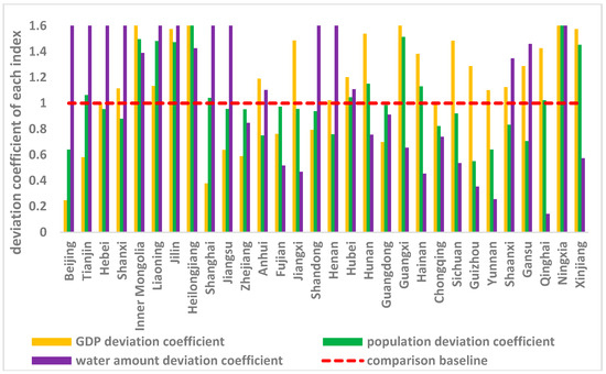
Figure 2.
Province deviation coefficient of each index.
From Figure 2 we can see that during the period from 2000 to 2015, only Zhejiang, Fujian, Guangdong, and Chongqing had COD emissions levels that correspond with low values of the three deviation coefficients. All three deviation coefficients were larger for Inner Mongolia, Liaoning, Jilin, Heilongjiang, Hubei, and Ningxia.
Each province’s difference score (Di) shown in Table 1 indicates heterogeneity among the provinces. It not only includes the historical responsibility each province should bear, but also contains the information on GDP, population, and water capital difference among the provinces. In order to calculate this, the three indices’ historical features need to be combined into one comprehensive value for decision making. The weight assigned by the information entropy method to GDP, population, and water capital are 0.55, 0.28, and 0.17, respectively. With each province’s historical data of these three factors, each factor’s contribution to the wastewater discharge permit allocation difference score was calculated and the spatial trend is shown in Figure 3 (detailed results are included in the Appendix Table A4).
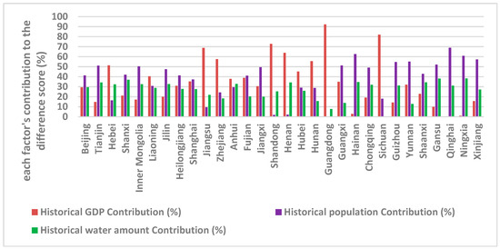
Figure 3.
The contribution of GDP, population, and water capital to the allocation score.
In our proposed allocation method, Hebei, Liaoning, Jiangsu, Zhejiang, Anhui, Shandong, Henan, Hubei, Hunan, Guangdong, and Sichuan provinces’ allocations are mainly influenced by their GDP history. The other 19 provinces’ allocations are highly impacted by their population growth. The water capital of each province did not impact the allocation of the permits significantly for all provinces. In addition, it is important to keep in mind that each index’s weight could change if the study period is extended. Hence, the proposed allocation framework is flexible and the allocations from it can be adjusted through time.
3.2. Comparison of Results with Those from Alternative Methods
The allocation method integrated with emission history proposed in this paper contains the following two main pieces of information: (1) Differences among provinces in terms of GDP population number and water capital; (2) Disparities among the provinces in terms of historical emission responsibilities. By comparing the results with those obtained from alternative methods and the central government’s allocation plan, we can get a deeper understanding of the differences in the disparities between the results of the different allocation methods. The comparative results are shown in Figure 4 and each province’s emission amount and reduction rate can be found in Appendix Table A5.
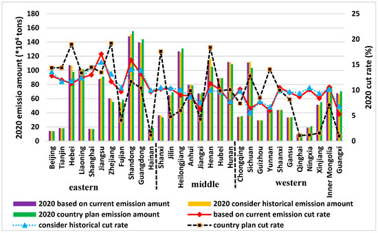
Figure 4.
Chemical oxygen demand (COD) discharge permits and emission reduction rate for the target year 2020 from different allocation plans.
From Figure 4, we find that the emission cut rates’ lines are gentler for the methods based on current emissions. The eastern part of China’s emission cut-rate is relatively higher than the middle and western part of the country for the method based on current emission trends and for the proposed one. The country plan methods give excessively small reduction rates for the western part of China. Provinces like Qinghai, Ningxia, and Xinjiang, which are the sources of China’s major rivers, benefit from this trend. The differences among the different allocation plans in terms of emission amount are negligible. Figure 5a shows the proposed mechanism difference among the allocation outputs in terms of the reduction rate. If the results from the allocation that considers emission history is higher than the one that does not, it indicates that these provinces had already historically enjoyed lower COD emission costs. The lower reduction rate results from the distribution mechanism that takes the emission history of the provinces into account mean that these provinces need higher pollution permits to take their economy a step forward. Provinces with bigger emission reduction rates are mostly in southern China, or in water-scarce regions of China like Beijing city, Tianjin city, and Hebei Province.

Figure 5.
The difference in COD cut-rate with different methods. Map generated with ArcGIS 10.6 for desktop (http://www.esri.com/sofware/arcgis).
The difference between the reduction rates from the allocation scheme that considers emission history and the one that does not is presented in Figure 5b. The Chinese government’s reduction plan usually considers each province’s economy and uses a uniform reduction rate [6,7]. Figure 5b shows that the reduction rate from our proposed method differs from the country plan. Let’s take Jilin and Zhejiang province in northeastern China as an example. As an industrial base for the time period 2000–2015, Jilin has a COD emission percentage increase of approximately 4.9% to 5.3% every year. Compared to Zhejiang’ reduction rate, the country plan allocates a smaller reduction rate to Jilin.
Figure 6a shows the difference in terms of emission amount from allocation schemes that do and do not take the emission history of the provinces and the country plan. By comparing the reduction rate of the current and historical scenarios, the government can approximate the historical responsibility of each region and determine whether each region’s rate of discharge should decrease or not. We took Guangdong, Guangxi, Ningxia, and Jiangsu as representative provinces for deeper analysis because these provinces’ allocations from these schemes differ greatly. Guangdong is a developed province and Guangxi is an underdeveloped province. According to the “Sustainable Cities in China”, 2016 report, these two provinces’ capital cities have severe water pollution problems which are affecting their sustainable development. However, under the country plan, both them do not have high COD reduction rates.
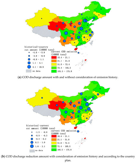
Figure 6.
The difference in COD cuts with different methods. Map generated with ArcGIS 10.6 for desktop (http://www.esri.com/sofware/arcgis).
Ningxia, in the western part of China, is one of the most water-scarce provinces [36]. The population of this province is low, therefore the discharge quota should be low and the reduction rate should be higher because the region does not have large assimilation capacity. However, the country plan only considers the GDP and assigns a very low reduction rate to this region. On the other hand, the Jiangsu Province is one of the most developed provinces, known for high industrial output. In 2007, the province had a serious water pollution incident [37]. With its recent rapid development, the province currently emits a huge amount of wastewater [38,39]. Considering this, the method we proposed allocated a lower emission permit to this province.
The proposed way of allocating emission permits could improve water quality, while providing equal development opportunities to the different regions. In addition, the proposed method can improve each province’s economic development potential as well as environmental quality. The proposed discharge permit allocation scheme should be complemented by building an effective emissions trading market to achieve even greater redistribution of total water pollution permits.
4. Conclusions
When allocating wastewater discharge permits, only considering each region’s current socioeconomic and environmental status is unfair because some regions have historically enjoyed low-cost pollution. This paper uses a new framework which considers each province’s economic, social, and environmental status together with emission history, to allocate China’s total COD discharge permits among its 30 provinces.
The main conclusions extracted from the results of this study are the following. (1) Most western regions with poor economic status, such as Yunnan, Sichuan, and Guizhou, have small emission reductions, which means these provinces will be given higher discharge limits. (2) Industrial provinces, such as Jiangsu, Shandong, Guangdong, Liaoning, and Zhejiang, will be allocated high emission reduction rates. This is a way makes these provinces take responsibility for their high emissions in the past. (3) The economically developed provinces, such as Beijing, Tianjin, and Shanghai, should cut their emissions even further. Because these provinces have the higher economic capacity, making cuts can be affordable for them.
There is still much research needed in this area, for example, identifying a finer scale (province-basin level) for water pollution permit distribution that is relevant to each province’s water quality situation. In the future, our methodologies could also be applied to other wastewater discharges pollutants (for example N, P, BOD, or TOC).
Overall, we hope that this research provides valuable insights that can help the country’s policy-makers make sustainable, efficient, and fair emission reduction decisions.
Author Contributions
J.H. and D.M.D. proposed the research ideas and methods of the manuscript and writing, V.B., W.H. and Z.Y. put forward the revise suggestion to the paper. M.A. are responsible for data collection and creating the figures and forms.
Funding
The study is supported by National Natural Science Foundation of China (No. 71471102).
Conflicts of Interest
The authors declare no conflict of interest.
Appendix A
Table A1.
Province deviation coefficient calculation based on GDP.
Table A1.
Province deviation coefficient calculation based on GDP.
| Region | Historical Accumulated GDP Value (×100 Million Yuan) | Proportion of Historical Accumulated GDP Value | Historical Accumulated COD Emission (×104 of Tons) | Proportion of History Accumulated COD Emission | GDP Deviation Coefficient |
|---|---|---|---|---|---|
| Beijing | 68,487.332 | 0.035 | 227.680 | 0.009 | 0.247 |
| Tianjin | 33,307.772 | 0.017 | 259.640 | 0.010 | 0.580 |
| Hebei | 101,389.733 | 0.051 | 1355.520 | 0.051 | 0.994 |
| Shanxi | 40,971.367 | 0.021 | 613.620 | 0.023 | 1.114 |
| Inner Mongolia | 33,377.821 | 0.017 | 739.150 | 0.028 | 1.646 |
| Liaoning | 84,709.411 | 0.043 | 1290.640 | 0.049 | 1.133 |
| Jilin | 38,398.277 | 0.019 | 813.390 | 0.031 | 1.575 |
| Heilongjiang | 54,837.166 | 0.028 | 1279.090 | 0.048 | 1.734 |
| Shanghai | 85,952.625 | 0.044 | 436.710 | 0.016 | 0.378 |
| Jiangsu | 173,625.790 | 0.088 | 1489.130 | 0.056 | 0.638 |
| Zhejiang | 125,655.584 | 0.064 | 996.290 | 0.037 | 0.589 |
| Anhui | 57,896.228 | 0.029 | 926.530 | 0.035 | 1.190 |
| Fujian | 69,822.310 | 0.035 | 714.480 | 0.027 | 0.761 |
| Jiangxi | 42,382.114 | 0.021 | 847.040 | 0.032 | 1.486 |
| Shandong | 167,440.987 | 0.085 | 1787.050 | 0.067 | 0.794 |
| Henan | 105,801.436 | 0.054 | 1455.110 | 0.055 | 1.023 |
| Hubei | 75,082.773 | 0.038 | 1212.740 | 0.046 | 1.201 |
| Hunan | 73,901.622 | 0.037 | 1529.710 | 0.058 | 1.539 |
| Guangdong | 207,160.428 | 0.105 | 1947.250 | 0.073 | 0.699 |
| Guangxi | 43,694.758 | 0.022 | 1458.590 | 0.055 | 2.482 |
| Hainan | 10,464.425 | 0.005 | 194.460 | 0.007 | 1.382 |
| Chongqing | 35,612.424 | 0.018 | 477.880 | 0.018 | 0.998 |
| Sichuan | 77,807.276 | 0.039 | 1552.600 | 0.058 | 1.484 |
| Guizhou | 23,442.067 | 0.012 | 405.910 | 0.015 | 1.287 |
| Yunnan | 39,617.141 | 0.020 | 586.700 | 0.022 | 1.101 |
| Shaanxi | 41,425.898 | 0.021 | 626.320 | 0.024 | 1.124 |
| Gansu | 21,096.297 | 0.011 | 365.270 | 0.014 | 1.287 |
| Qinghai | 5978.322 | 0.003 | 114.670 | 0.004 | 1.426 |
| Ningxia | 7400.343 | 0.004 | 255.330 | 0.010 | 2.565 |
| Xinjiang | 29,119.675 | 0.015 | 616.820 | 0.023 | 1.575 |
| Sum | 1,975,859 | 1 | 26575.32 | 1 | - |
Note. Based on historical GDP and COD data and Equations (1)–(3), we calculated the GDP deviation coefficient.
Table A2.
Population deviation coefficient calculation.
Table A2.
Population deviation coefficient calculation.
| Region | History Accumulated Population Value (×104 Person) | Proportion of History Accumulated Population Value | History Accumulated COD Emission (×104 Tons) | Proportion of History Accumulated COD Emission | Population Deviation Coefficient |
|---|---|---|---|---|---|
| Beijing | 28,055 | 0.013 | 227.68 | 0.009 | 0.641 |
| Tianjin | 19,287 | 0.009 | 259.64 | 0.010 | 1.063 |
| Hebei | 112,266 | 0.053 | 1355.52 | 0.051 | 0.954 |
| Shanxi | 55,143 | 0.026 | 613.62 | 0.023 | 0.879 |
| Inner Mongolia | 39,023 | 0.019 | 739.15 | 0.028 | 1.496 |
| Liaoning | 68,764 | 0.033 | 1290.64 | 0.049 | 1.482 |
| Jilin | 43,630 | 0.021 | 813.39 | 0.031 | 1.472 |
| Heilongjiang | 61,162 | 0.029 | 1279.09 | 0.048 | 1.652 |
| Shanghai | 33,146 | 0.016 | 436.71 | 0.016 | 1.041 |
| Jiangsu | 123,175 | 0.059 | 1489.13 | 0.056 | 0.955 |
| Zhejiang | 82,605 | 0.039 | 996.29 | 0.037 | 0.953 |
| Anhui | 97,540 | 0.046 | 926.53 | 0.035 | 0.750 |
| Fujian | 58,001 | 0.028 | 714.48 | 0.027 | 0.973 |
| Jiangxi | 70,029 | 0.033 | 847.04 | 0.032 | 0.955 |
| Shandong | 150,516 | 0.072 | 1787.05 | 0.067 | 0.938 |
| Henan | 151,616 | 0.072 | 1455.11 | 0.055 | 0.758 |
| Hubei | 91,624 | 0.044 | 1212.74 | 0.046 | 1.045 |
| Hunan | 104,973 | 0.050 | 1529.71 | 0.058 | 1.151 |
| Guangdong | 156,375 | 0.075 | 1947.25 | 0.073 | 0.984 |
| Guangxi | 76,132 | 0.036 | 1458.59 | 0.055 | 1.513 |
| Hainan | 13,586 | 0.006 | 194.46 | 0.007 | 1.130 |
| Chongqing | 45,935 | 0.022 | 477.88 | 0.018 | 0.822 |
| Sichuan | 133,330.9 | 0.064 | 1552.6 | 0.058 | 0.920 |
| Guizhou | 58,323 | 0.028 | 405.91 | 0.015 | 0.550 |
| Yunnan | 72,248 | 0.034 | 586.7 | 0.022 | 0.641 |
| Shaanxi | 59,417 | 0.028 | 626.32 | 0.024 | 0.833 |
| Gansu | 40,868 | 0.019 | 365.27 | 0.014 | 0.706 |
| Qinghai | 8849 | 0.004 | 114.67 | 0.004 | 1.023 |
| Ningxia | 9813 | 0.005 | 255.33 | 0.010 | 2.055 |
| Xinjiang | 33,521 | 0.016 | 616.82 | 0.023 | 1.453 |
| Sum | 2,098,953 | 1.000 | 26,575.32 | 1.000 | - |
Table A3.
Water capital deviation coefficient calculation.
Table A3.
Water capital deviation coefficient calculation.
| Region | History Accumulated Water Capital Value (×108 Cubic Meter) | Proportion of History Accumulated Water Capital Value | History Accumulated COD Emission (×104 Tons) | Proportion of History Accumulated COD Emission | Water Capital Deviation Coefficient |
|---|---|---|---|---|---|
| Beijing | 378.32 | 0.001 | 227.68 | 0.009 | 8.215 |
| Tianjin | 199.32 | 0.001 | 259.64 | 0.010 | 17.782 |
| Hebei | 2260.62 | 0.006 | 1355.52 | 0.051 | 8.185 |
| Shanxi | 1560.51 | 0.004 | 613.62 | 0.023 | 5.368 |
| Inner Mongolia | 7264.67 | 0.020 | 739.15 | 0.028 | 1.389 |
| Liaoning | 4619.5 | 0.013 | 1290.64 | 0.049 | 3.814 |
| Jilin | 6372.08 | 0.018 | 813.39 | 0.031 | 1.743 |
| Heilongjiang | 12,246.1 | 0.034 | 1279.09 | 0.048 | 1.426 |
| Shanghai | 556.47 | 0.002 | 436.71 | 0.016 | 10.713 |
| Jiangsu | 6454.73 | 0.018 | 1489.13 | 0.056 | 3.149 |
| Zhejiang | 16,036.7 | 0.044 | 996.29 | 0.037 | 0.848 |
| Anhui | 11,475.66 | 0.032 | 926.53 | 0.035 | 1.102 |
| Fujian | 18,916.38 | 0.052 | 714.48 | 0.027 | 0.516 |
| Jiangxi | 24,678.45 | 0.068 | 847.04 | 0.032 | 0.469 |
| Shandong | 4583.72 | 0.013 | 1787.05 | 0.067 | 5.322 |
| Henan | 6263.97 | 0.017 | 1455.11 | 0.055 | 3.171 |
| Hubei | 14,928.7 | 0.041 | 1212.74 | 0.046 | 1.109 |
| Hunan | 27,604.61 | 0.076 | 1529.71 | 0.058 | 0.756 |
| Guangdong | 29,139.17 | 0.080 | 1947.25 | 0.073 | 0.912 |
| Guangxi | 30,383.02 | 0.084 | 1458.59 | 0.055 | 0.655 |
| Hainan | 5848.6 | 0.016 | 194.46 | 0.007 | 0.454 |
| Chongqing | 8812.11 | 0.024 | 477.88 | 0.018 | 0.740 |
| Sichuan | 39,638.64 | 0.109 | 1552.6 | 0.058 | 0.535 |
| Guizhou | 15,651.39 | 0.043 | 405.91 | 0.015 | 0.354 |
| Yunnan | 31,253.32 | 0.086 | 586.7 | 0.022 | 0.256 |
| Shaanxi | 6340.89 | 0.017 | 626.32 | 0.024 | 1.348 |
| Gansu | 3415.3 | 0.009 | 365.27 | 0.014 | 1.460 |
| Qinghai | 11,050.8 | 0.030 | 114.67 | 0.004 | 0.142 |
| Ningxia | 159.741 | 0.000 | 255.33 | 0.010 | 21.820 |
| Xinjiang | 14,683.12 | 0.040 | 616.82 | 0.023 | 0.573 |
| Sum | 362,776.6 | 1.000 | 26,575.32 | 1.000 | - |
Table A4.
Each factor’s contribution to the allocation difference score in each province.
Table A4.
Each factor’s contribution to the allocation difference score in each province.
| Region | Historical GDP Contribution (%) | Historical Population Contribution (%) | Historical Water Capital Contribution (%) |
|---|---|---|---|
| Beijing | 29.3 | 41.3 | 29.5 |
| Tianjin | 14.8 | 51.0 | 34.2 |
| Hebei | 51.4 | 16.3 | 32.3 |
| Shanxi | 21.1 | 42.0 | 36.9 |
| Inner Mongolia | 17.1 | 50.4 | 32.5 |
| Liaoning | 40.4 | 30.8 | 28.8 |
| Jilin | 19.9 | 47.4 | 32.7 |
| Heilongjiang | 30.9 | 41.3 | 27.8 |
| Shanghai | 35.2 | 37.2 | 27.6 |
| Jiangsu | 68.8 | 9.4 | 21.8 |
| Zhejiang | 57.5 | 24.3 | 18.2 |
| Anhui | 37.8 | 29.4 | 32.8 |
| Fujian | 38.8 | 41.0 | 20.2 |
| Jiangxi | 30.4 | 49.5 | 20.0 |
| Shandong | 72.8 | 1.8 | 25.3 |
| Henan | 63.8 | 2.1 | 34.2 |
| Hubei | 45.1 | 29.0 | 25.9 |
| Hunan | 55.5 | 28.8 | 15.7 |
| Guangdong | 92.3 | 0.0 | 7.7 |
| Guangxi | 35.0 | 51.2 | 13.8 |
| Hainan | 2.9 | 62.6 | 34.6 |
| Chongqing | 19.1 | 49.0 | 31.9 |
| Sichuan | 82.0 | 18.0 | 0.0 |
| Guizhou | 14.2 | 54.6 | 31.2 |
| Yunnan | 32.1 | 55.1 | 12.8 |
| Shaanxi | 22.8 | 42.8 | 34.3 |
| Gansu | 9.9 | 52.0 | 38.1 |
| Qinghai | 0.0 | 68.9 | 31.1 |
| Ningxia | 0.9 | 60.9 | 38.3 |
| Xinjiang | 15.7 | 57.2 | 27.1 |
Table A5.
COD discharge amounts in 2015 and 2020 and discharge reduction proportion.
Table A5.
COD discharge amounts in 2015 and 2020 and discharge reduction proportion.
| Region | Discharge Amount (×104 Tons) in 2015 | 2020 Based on Current Emission | 2020 Consider Historical | 2020 Country Plan | |||
|---|---|---|---|---|---|---|---|
| Emission Amount (×104 Tons) | Cut Rate (%) | Emission Amount (×104 Tons) | Cut Rate (%) | Emission Amount (×104 Tons) | Cut Rate (%) | ||
| Beijing | 16.2 | 14.1 | 12.8 | 14.0 | 13.6 | 13.9 | 14.4 |
| Tianjin | 20.9 | 18.4 | 12.0 | 18.4 | 11.7 | 17.9 | 14.4 |
| Hebei | 120.8 | 107.1 | 11.3 | 106.5 | 11.8 | 97.8 | 19 |
| Shanxi | 40.5 | 36.4 | 10.2 | 36.2 | 10.5 | 33.4 | 17.6 |
| Inner Mongolia | 83.6 | 74.7 | 10.6 | 75.1 | 10.2 | 77.7 | 7.1 |
| Liaoning | 116.7 | 102.2 | 12.4 | 102.2 | 12.4 | 101.1 | 13.4 |
| Jilin | 72.4 | 64.9 | 10.3 | 64.9 | 10.4 | 68.9 | 4.8 |
| Heilongjiang | 139.3 | 126.8 | 9.0 | 125.3 | 10.1 | 130.9 | 6 |
| Shanghai | 19.9 | 17.3 | 13.0 | 17.0 | 14.5 | 17.0 | 14.5 |
| Jiangsu | 105.5 | 87.5 | 17.1 | 89.2 | 15.5 | 91.3 | 13.5 |
| Zhejiang | 68.3 | 60.3 | 11.7 | 59.3 | 13.2 | 55.2 | 19.2 |
| Anhui | 87.1 | 79.4 | 8.9 | 79.5 | 8.7 | 78.5 | 9.9 |
| Fujian | 60.9 | 55.0 | 9.7 | 54.5 | 10.5 | 58.4 | 4.1 |
| Jiangxi | 71.6 | 67.1 | 6.3 | 66.2 | 7.6 | 68.5 | 4.3 |
| Shandong | 175.8 | 147.9 | 15.9 | 151.0 | 14.1 | 155.2 | 11.7 |
| Henan | 128.7 | 114.2 | 11.3 | 115.9 | 10.0 | 105.0 | 18.4 |
| Hubei | 98.6 | 88.7 | 10.1 | 89.0 | 9.7 | 88.8 | 9.9 |
| Hunan | 120.8 | 111.7 | 7.6 | 111.4 | 7.8 | 108.6 | 10.1 |
| Guangdong | 160.7 | 139.4 | 13.2 | 138.4 | 13.9 | 144.0 | 10.4 |
| Guangxi | 71.1 | 67.4 | 5.3 | 66.2 | 6.8 | 70.4 | 1 |
| Hainan | 18.8 | 17.0 | 9.7 | 16.9 | 10.0 | 18.6 | 1.2 |
| Chongqing | 38 | 34.1 | 10.2 | 34.3 | 9.8 | 35.2 | 7.4 |
| Sichuan | 118.6 | 111.0 | 6.4 | 112.0 | 5.6 | 103.4 | 12.8 |
| Guizhou | 31.8 | 29.4 | 7.6 | 29.3 | 7.8 | 29.1 | 8.5 |
| Yunnan | 51 | 48.0 | 6.0 | 47.6 | 6.7 | 43.8 | 14.1 |
| Shaanxi | 48.9 | 43.8 | 10.5 | 44.1 | 9.9 | 44.0 | 10 |
| Gansu | 36.6 | 33.1 | 9.5 | 33.1 | 9.7 | 33.6 | 8.2 |
| Qinghai | 10.4 | 9.5 | 8.7 | 9.4 | 9.4 | 10.3 | 1.1 |
| Ningxia | 21.1 | 19.0 | 10.1 | 18.9 | 10.5 | 20.8 | 1.2 |
| Xinjiang | 56 | 51.3 | 8.4 | 50.7 | 9.4 | 55.1 | 1.6 |
| Sum | 2210.6 | 1976.7 | - | 1976.5 | - | 1976.4 | - |
Note. Whole China COD emission in 2015 is 2213.5 × 104 tons, The Discharge amount (×104 tons) in 2015 here are not include Tibet (2.88 × 10⁴ tons) data. The cut rate (reduction rate) means the proportion of average COD amount one province need to cut in 2016–2020 compared with its 2015 COD emission.
References
- Zhang, Y.; Fu, G.; Yu, T.; Shen, M.; Meng, W.; Ongley, E.D. Trans-jurisdictional pollution control options within an integrated water resources management framework in water-scarce north-eastern China. Water Policy 2011, 13, 624–644. [Google Scholar] [CrossRef]
- Lung, W.S. Water Quality Modeling for Wasteload Allocation and TMDLs; John Wiley & Sons: Hoboken, NJ, USA, 2001. [Google Scholar]
- Linker, L.C.; Batiuk, R.A.; Shenk, G.W.; Cerco, C.F. Development of the Chesapeake Bay watershed total maximum daily load allocation. J. Am. Water Resour. Assoc. 2013, 49, 986–1006. [Google Scholar] [CrossRef]
- Takeoka, H. Progress in Seto Inland Sea research. J. Oceanogr. 2002, 58, 93–107. [Google Scholar] [CrossRef]
- Kataoka, Y. Water quality management in Japan:Recent Developments and Challenges for Integration. Environ. Policy Gov. 2011, 21, 338–350. [Google Scholar] [CrossRef]
- Sun, T.; Zhang, H.; Wang, Y.; Meng, X.; Wang, C. The application of environmental Gini coefficient (EGC) in allocating wastewater discharge permit: The case study of watershed total mass control in Tianjin, China. Resour. Conserv. Recycl. 2010, 54, 601–608. [Google Scholar] [CrossRef]
- Yuan, Q.; McIntyre, N.; Wu, Y.; Liu, Y.; Liu, Y. Towards greater socio-economic equality in allocation of wastewater discharge permits in China based on the weighted Gini coefficient. Resour. Conserv. Recycl. 2017, 127, 196–205. [Google Scholar] [CrossRef]
- Sado, Y.; Boisvert, R.N.; Poe, G.L. Potential cost savings from discharge allowance trading: A case study and implications for water quality trading. Water Resour. Res. 2010, 46, 1–12. [Google Scholar] [CrossRef]
- Prabodanie, R.A.R.; Raffensperger, J.F.; Milke, M.W. A pollution offset system for trading non-point source water pollution Permits. Environ. Resour. Econ. 2010, 45, 499–515. [Google Scholar] [CrossRef]
- James Shortle Economics and environmental markets:lessons from water-quality trading. Agric. Resour. Econ. Rev. 2013, 42, 57–74. [CrossRef]
- Fisher-vanden, K.; Olmstead, S. Moving pollution trading from Air to Water: Potential, Problems, and Prognosis. J. Econ. Perspect. 2013, 27, 147–172. [Google Scholar] [CrossRef]
- Hung, M.F.; Shaw, D. A trading-ratio system for trading water pollution discharge permits. J. Environ. Econ. Manag. 2005, 49, 83–102. [Google Scholar] [CrossRef]
- Niksokhan, M.H.; Kerachian, R.; Amin, P. A stochastic conflict resolution model for trading pollutant discharge permits in river systems. Environ. Monit. Assess. 2009, 154, 219–232. [Google Scholar] [CrossRef] [PubMed]
- Sun, T.; Zhang, H.; Wang, Y. The application of information entropy in basin level water waste permits allocation in China. Resour. Conserv. Recycl. 2013, 70, 50–54. [Google Scholar] [CrossRef]
- Nikoo, M.R.; Kerachian, R.; Karimi, A. A Nonlinear Interval Model for Water and Waste Load Allocation in River Basins. Water Resour. Manag. 2012, 26, 2911–2926. [Google Scholar] [CrossRef]
- Mahjouri, N.; Bizhani-Manzar, M. Waste Load Allocation in Rivers using Fallback Bargaining. Water Resour. Manag. 2013, 27, 2125–2136. [Google Scholar] [CrossRef]
- Qin, X.; Huang, G.; Chen, B.; Zhang, B. An interval-parameter waste-load-allocation model for river water quality management under uncertainty. Environ. Manag. 2009, 43, 999–1012. [Google Scholar] [CrossRef] [PubMed]
- Gosseries, A. Historical emissions and free riding. Ethical Perspect. 2004, 11, 36–60. [Google Scholar] [CrossRef]
- Pan, J.; Phillips, J.; Chen, Y. China’s balance of emissions embodied in trade: Approaches to measurement and allocating international responsibility. Oxf. Rev. Econ. Policy 2008, 24, 354–376. [Google Scholar] [CrossRef]
- Friman, M.; Strandberg, G. Historical responsibility for climate change: Science and the science-policy interface. Wiley Interdiscip. Rev. Clim. Chang. 2014, 5, 297–316. [Google Scholar] [CrossRef]
- Den Elzen, M.G.J.; Schaeffer, M.; Lucas, P.L. Differentiating future commitments on the basis of countries’ relative historical responsibility for climate change: Uncertainties in the “Brazilian Proposal” in the context of a policy implementation. Clim. Chang. 2005, 71, 277–301. [Google Scholar] [CrossRef]
- Fischer, C.; Fox, A. Output-Based Allocations of Emissions Permits: Efficiency and Distributional Effects in a General Equilibrium Setting with Taxes and Trade; Resource for the Future: Washington, DC, USA, 2004. [Google Scholar]
- Liao, Z.; Zhu, X.; Shi, J. Case study on initial allocation of Shanghai carbon emission trading based on Shapley value. J. Clean. Prod. 2015, 103, 338–344. [Google Scholar] [CrossRef]
- Mackenzie, I.A.; Hanley, N.; Kornienko, T. A Permit Allocation Contest for a Tradable Pollution Permit Market (March 2008). CER-ETH—Center of Economic Research at ETH Zurich, Working Paper No. 08/82. Available online: https://ssrn.com/abstract=1102217 (accessed on 10 December 2018).
- Lu, Y.; Song, S.; Wang, R.; Liu, Z.; Meng, J.; Sweetman, A.J.; Jenkins, A.; Ferrier, R.C.; Li, H.; Luo, W.; et al. Impacts of soil and water pollution on food safety and health risks in China. Environ. Int. 2015, 77, 5–15. [Google Scholar] [CrossRef] [PubMed]
- Démurger, S. Infrastructure Development and Economic Growth: An Explanation for Regional Disparities in China? J. Comp. Econ. 2001, 29, 95–117. [Google Scholar] [CrossRef]
- Kanbur, R.; Zhang, X. Fifty years of regional inequality in China: A journey through central planning, reform, and openness. Reg. Inequal. China Trends Explan. Policy Responses 2009, 9, 45–63. [Google Scholar] [CrossRef]
- National Bureau of Statistics of China. China Statistics Yearbook (2000–2015); China Statistica Press: Beijing, China, 2000–2015.
- National Bureau of Statistics of China; Ministry of Environmental Protection of China. China Statistic Yearbook on Environment (2011–2015); China Statistica Press: Beijing, China, 2015.
- National Bureau of Statistics of China. China Water Resources Bulletin (2000-2015); China Water & Power Press: Beijing, China, 2000–2015.
- Wu, Y.; Zhou, Y.; Saveriades, G.; Agaian, S.; Noonan, J.P.; Natarajan, P. Local Shannon entropy measure with statistical tests for image randomness. Inf. Sci. 2013, 222, 323–342. [Google Scholar] [CrossRef]
- Singh, V.P.; Asce, F. Hydrologic Synthesis Using Entropy Theory: Review. J. Hydrol. Eng. 2011, 16, 421–433. [Google Scholar] [CrossRef]
- Zou, Z.-H.; Yun, Y.; Sun, J.-N. Entropy method for determination of weight of evaluating indicators in fuzzy synthetic evaluation for water quality assessment. J. Environ. Sci. 2006, 18, 1020–1023. [Google Scholar] [CrossRef]
- Shyu, G.S.; Cheng, B.Y.; Chiang, C.T.; Yao, P.H.; Chang, T.K. Applying factor analysis combined with kriging and information entropy theory for mapping and evaluating the stability of groundwater quality variation in Taiwan. Int. J. Environ. Res. Public Health 2011, 8, 1084–1109. [Google Scholar] [CrossRef]
- Liu, D.; Li, L. Application Study of Comprehensive Forecasting Model Based on Entropy Weighting Method on Trend of PM2.5 Concentration in Guangzhou, China. Int. J. Environ. Res. Public Health 2015, 12, 7085–7099. [Google Scholar] [CrossRef]
- Bao, C.; Zou, J. Exploring the coupling and decoupling relationships between urbanization quality and water resources constraint intensity: Spatiotemporal analysis for northwest China. Sustainability 2017, 9, 1960. [Google Scholar] [CrossRef]
- Qin, B.; Xu, P.; Wu, Q.; Luo, L.; Yun, Z. Environmental issues of lake Taihu, China. Hydrobiologia 2007, 581, 3–14. [Google Scholar] [CrossRef]
- Xie, R.; Pang, Y.; Kun, B. Spatiotemporal distribution of water environmental capacity-a case study on the western areas of Taihu Lake in Jiangsu Province, China. Environ. Sci. Pollut. Res. 2014, 21, 5465–5473. [Google Scholar] [CrossRef] [PubMed]
- Rajeshkumar, S.; Liu, Y.; Zhang, X.; Ravikumar, B.; Bai, G.; Li, X. Studies on seasonal pollution of heavy metals in water, sediment, fish and oyster from the Meiliang Bay of Taihu Lake in China. Chemosphere 2018, 191, 626–638. [Google Scholar] [CrossRef] [PubMed]
© 2018 by the authors. Licensee MDPI, Basel, Switzerland. This article is an open access article distributed under the terms and conditions of the Creative Commons Attribution (CC BY) license (http://creativecommons.org/licenses/by/4.0/).