Entropy and Mutability for the q-State Clock Model in Small Systems
Abstract
1. Introduction
2. Model and Methods
2.1. General Definitions
2.2. Exact Theoretical Approach for a Small System
2.3. Numerical Simulations
2.4. Thermal Averages
2.5. Information Theory, Mutability, and Diversity
3. Results and Discussions
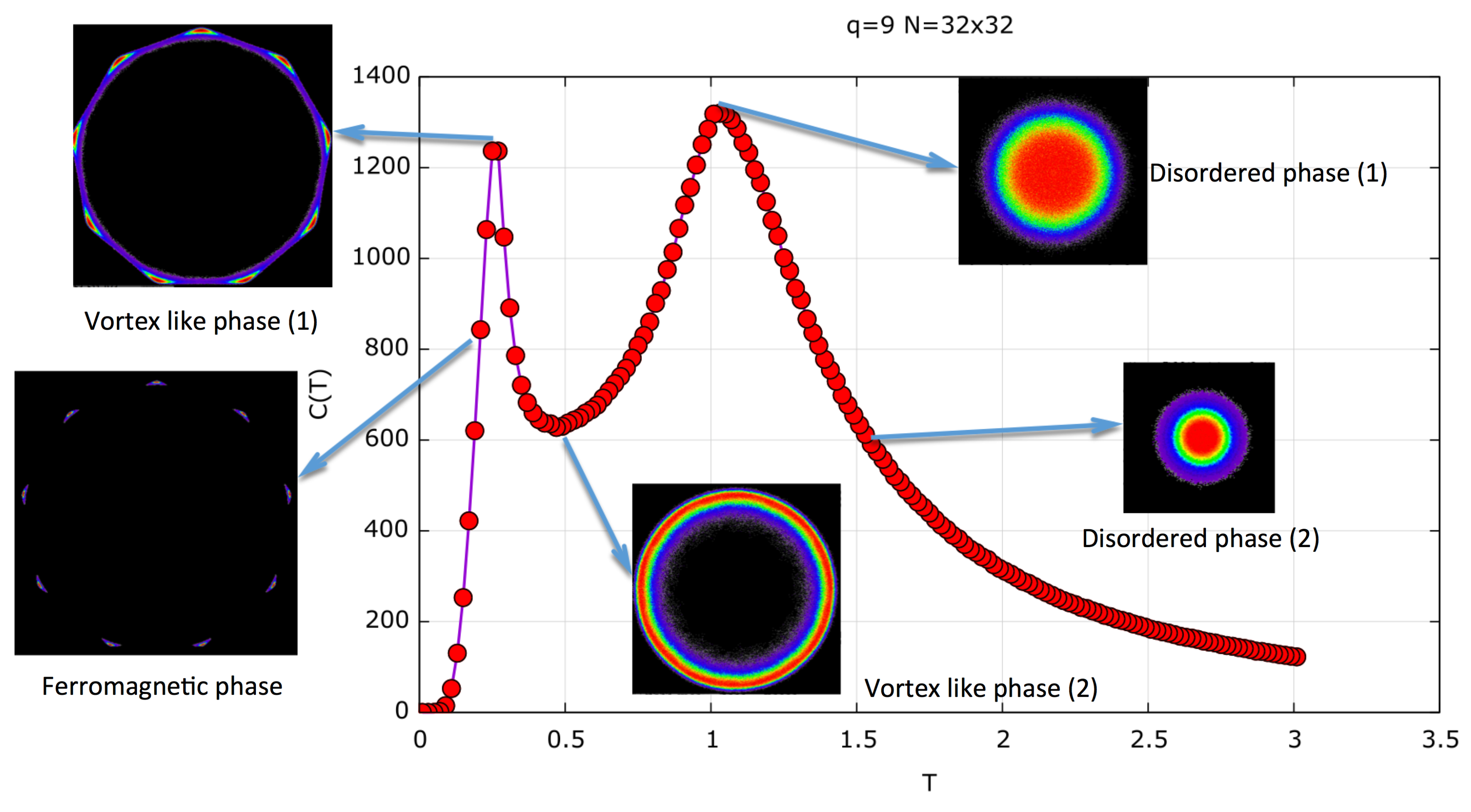
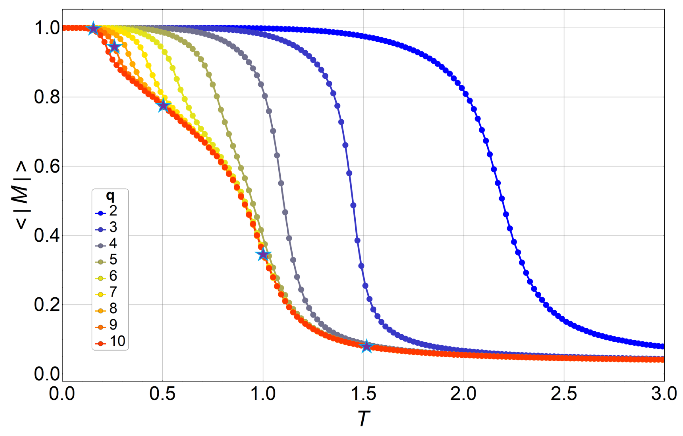
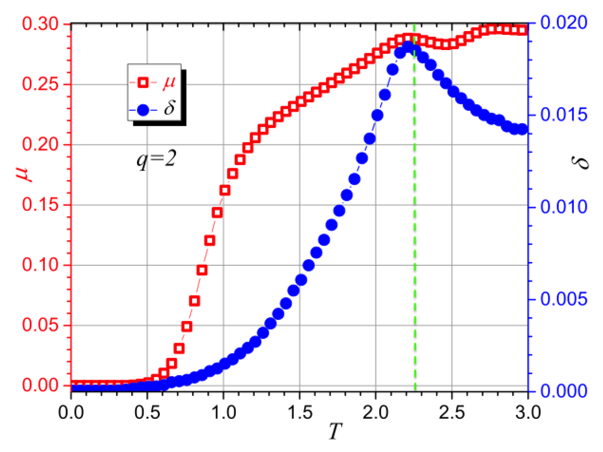
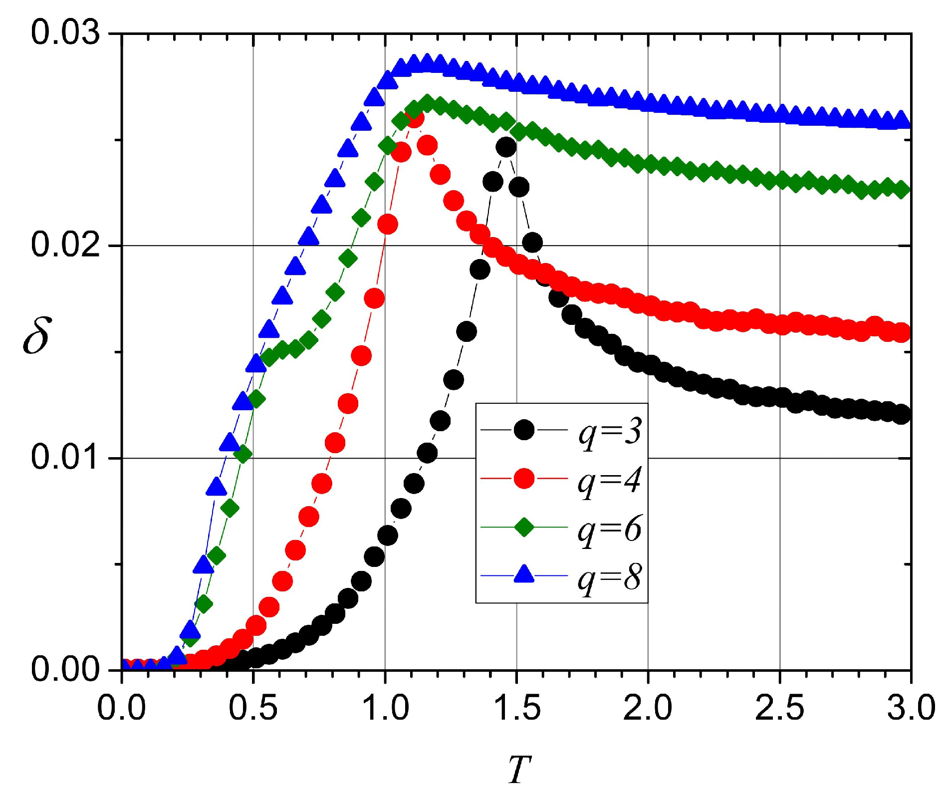
3.1. Monte Carlo Simulations
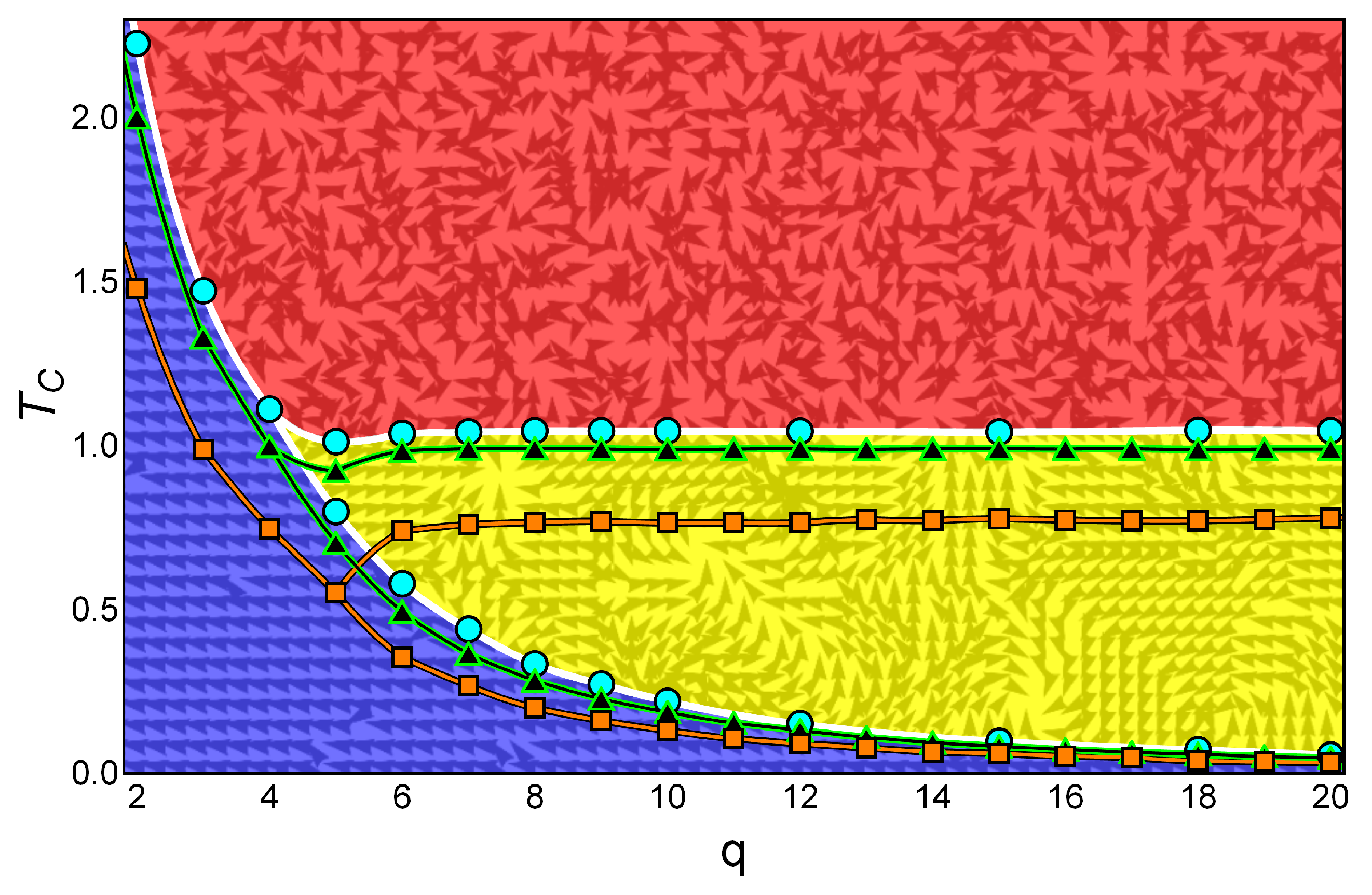
3.2. Phase Diagram
4. Conclusions
Author Contributions
Acknowledgments
Conflicts of Interest
References
- Berezinskii, V.L. Destruction of Long-range Order in One-dimensional and Two-dimensional Systems having a Continuous Symmetry Group I. Classical Systems. Zh. Eksp. Teor. Fiz. 1971, 59, 907–920. [Google Scholar]
- Kosterlitz, J.M.; Thouless, D.J. Long range order and metastability in two dimensional solids and superfluids. (Application of dislocation theory). J. Phys. C Solid State Phys. 1972, 5, L124. [Google Scholar] [CrossRef]
- Cardy, J.L.; Ostlund, S. Random symmetry-breaking fields and the XY model. Phys. Rev. B 1982, 25, 6899. [Google Scholar] [CrossRef]
- Doussal, P.L.; Giamarchi, T. Replica Symmetry Breaking Instability in the 2D XY Model in a Random Field. Phys. Rev. Lett. 1995, 74, 606. [Google Scholar] [CrossRef]
- Nobre, F.D.; Sherrington, D. The infinite-range clock spin glass model: An investigation of the relevance of reflection symmetry. J. Phys. C Solid State Phys. 1986, 19, L181. [Google Scholar] [CrossRef]
- Ilker, E.; Berker, A.N. High q-state clock spin glasses in three dimensions and the Lyapunov exponents of chaotic phases and chaotic phase boundaries. Phys. Rev. E 2013, 87, 032124. [Google Scholar] [CrossRef]
- Ilker, E.; Berker, A.N. Odd q-state clock spin-glass models in three dimensions, asymmetric phase diagrams, and multiple algebraically ordered phases. Phys. Rev. E 2014, 90, 062112. [Google Scholar] [CrossRef]
- Lupo, C.; Ricci-Tersenghi, F. Approximating the XY model on a random graph with a q-state clock model. Phys. Rev. B 2017, 95, 054433. [Google Scholar] [CrossRef]
- Kosterlitz, J.M.; Thouless, D.J. Ordering, metastability and phase transitions in two-dimensional systems. J. Phys. C Solid State Phys. 1973, 6, 1181–1203. [Google Scholar] [CrossRef]
- Kosterlitz, J.M. The critical properties of the two-dimensional XY model. J. Phys. C Solid State Phys. 1974, 7, 1046–1060. [Google Scholar] [CrossRef]
- Jose, J.V.; Kadanoff, L.P.; Kirkpatrick, S.; Nelson, D.R. Renormalization, vortices, and symmetry-breaking perturbations in the two-dimensional planar model. Phys. Rev. B 1977, 16, 1217–1241. [Google Scholar] [CrossRef]
- Kenna, R. The XY Model and the Berezinskii-Kosterlitz-Thouless Phase Transition. arXiv, 2005; arXiv:cond-mat/0512356. [Google Scholar]
- Jose, J.V. (Ed.) 40 Years of Berezinskii-Kosterlitz-Thouless Theory; World Scientific: London, UK, 2013. [Google Scholar]
- Elitzur, S.; Pearson, R.B.; Shigemitsu, J. Phase structure of discrete Abelian spin and gauge systems. Phys. Rev. D 1979, 19, 3698–3714. [Google Scholar] [CrossRef]
- Cardy, J.L. General discrete planar models in two dimensions: Duality properties and phase diagrams. J. Phys. A Math. Gen. 1980, 13, 1507–1515. [Google Scholar] [CrossRef]
- Fröhlich, J.; Spencer, T. The Kosterlitz-Thouless transition in two-dimensional Abelian spin systems and the Coulomb gas. Commun. Math. Phys. 1981, 81, 527–602. [Google Scholar] [CrossRef]
- Ortiz, G.; Cobanera, E.; Nussinov, Z. Dualities and the phase diagram of the p-clock model. Nucl. Phys. B 2012, 854, 780–814. [Google Scholar] [CrossRef]
- Kumano, Y.; Hukushima, K.; Tomita, Y.; Oshikawa, M. Response to a twist in systems with Zp symmetry: The two-dimensional p-state clock model. Phys. Rev. B 2013, 88, 104427. [Google Scholar] [CrossRef]
- Kim, D.H. Partition function zeros of the p-state clock model in the complex temperature plan. Phys. Rev. E 2017, 96, 052130. [Google Scholar] [CrossRef]
- Borisenko, O.; Cortese, G.; Fiore, R.; Gravina, M.; Papa, A. Numerical study of the phase transitions in the two-dimensional Z(5) vector model. Phys. Rev. E 2011, 83, 041120. [Google Scholar] [CrossRef]
- Vogel, E.E.; Saravia, G.; Bachmann, F.; Fierro, B.; Fischer, J. Phase transitions in Edwards-Anderson model by means of information theory. Physica A 2009, 388, 4075–4082. [Google Scholar] [CrossRef]
- Binder, K. Finite size scaling analysis of ising model block distribution functions. Z. Phys. B 1981, 119, 119–140. [Google Scholar] [CrossRef]
- Vogel, E.E.; Saravia, G.; Cortez, L.V. Data compressor designed to improve recognition of magnetic phases. Physica A 2012, 391, 1591–1601. [Google Scholar] [CrossRef]
- Cortez, L.V.; Saravia, G.; Vogel, E.E. Phase diagram and reentrance for the 3D Edwards-Anderson model using information theory. J. Magn. Magn. Mater. 2014, 372, 173–180. [Google Scholar] [CrossRef]
- Vogel, E.E.; Saravia, G. Information theory applied to econophysics: Stock market behaviors. Eur. Phys. J. B 2014, 87, 177. [Google Scholar] [CrossRef]
- Vogel, E.E.; Saravia, G.; Astete, J.; Diaz, J.; Riadi, F. Information theory as a tool to improve individual pensions: The Chilean case. Physica A 2015, 424, 372–382. [Google Scholar] [CrossRef]
- Contreras, D.J.; Vogel, E.E.; Saravia, G.; Stockins, B. Derivation of a measure of systolic blood pressure mutability: A novel information theory-based metric from ambulatory blood pressure tests. J. Am. Soc. Hypertens. 2016, 10, 217–223. [Google Scholar] [CrossRef]
- Vogel, E.E.; Saravia, G.; Pasten, D.; Munoz, V. Time-series analysis of earthquake sequences by means of information recognizer. Tectonophysics 2017, 712, 723–728. [Google Scholar] [CrossRef]
- Vogel, E.E.; Saravia, G.; Ramirez-Pastor, A.J. Phase diagrams in a system of long rods on two-dimensional lattices by means of information theory. Phys. Rev. E 2017, 96, 062133. [Google Scholar] [CrossRef]
- Vogel, E.E.; Saravia, G.; Kobe, S.; Schumann, R.; Schuster, R. A novel method to optimize electricity generation from wind energy. Renew. Energy 2018, 126, 724–735. [Google Scholar] [CrossRef]
- Baek, S.K.; Minnhagen, P.; Kim, B.J. True and quasi-long-range order in the generalized q-state clock model. Phys. Rev. E 2009, 80, 060101. [Google Scholar] [CrossRef]
- Onsager, L. Crystal statistics I. A two-dimensional model with an order-disorder transition. Phys. Rev. 1944, 65, 117. [Google Scholar] [CrossRef]



| n | |||||
|---|---|---|---|---|---|
| 1 | 4 | 6 | |||
| 2 | 32 | 48 | |||
| 3 | 128 | 192 | |||
| 4 | 248 | 348 | |||
| 5 | 896 | 960 | |||
| 6 | 2336 | 2448 | |||
| 7 | 4864 | 2736 | |||
| 8 | 10,748 | 5376 | |||
| 9 | 19,712 | 11,808 | |||
| 10 | 29,376 | 14,880 | |||
| 11 | 39,936 | 22,128 | |||
| 12 | 0 | 45,584 | 54,072 | ||
| 13 | 1 | 39,936 | 54,960 | ||
| 14 | 2 | 29,376 | 94,032 | ||
| 15 | 3 | 19,712 | 175,968 | ||
| 16 | 4 | 10,748 | 191,514 | ||
| 17 | 5 | 4864 | 231,744 | ||
| 18 | 6 | 2336 | 478,752 | ||
| 19 | 7 | 896 | 393,360 | ||
| 20 | 8 | 248 | 530,892 | ||
| 21 | 9 | 128 | 806,736 | ||
| 22 | 10 | 32 | 707,760 | ||
| 23 | 12 | 4 | 701,712 | ||
| 24 | 0 | 1,112,830 | |||
| n | |||||||||||
|---|---|---|---|---|---|---|---|---|---|---|---|
| n | n | n | |||||||||
| 1 | 5 | 23 | 15,760 | 45 | 15,760 | 67 | 2.30902 | 89,000 | |||
| 2 | 40 | 24 | 290 | 46 | 4100 | 68 | 2.47214 | 1340 | |||
| 3 | 160 | 25 | 6720 | 47 | 124,320 | 69 | 2.73607 | 58,080 | |||
| 4 | 290 | 26 | 8960 | 48 | 1680 | 70 | 3 | 30,200 | |||
| 5 | 800 | 27 | 30,360 | 49 | 27,920 | 71 | 3.16312 | 6720 | |||
| 6 | 40 | 28 | 680 | 50 | 57,000 | 72 | 3.42705 | 64,120 | |||
| 7 | 320 | 29 | 5280 | 51 | 117,040 | 73 | 3.8541 | 21,160 | |||
| 8 | 1680 | 30 | 23,080 | 52 | 6958 | 74 | 4.11803 | 23,640 | |||
| 9 | 680 | 31 | 410 | 53 | 9200 | 75 | 4.28115 | 1440 | |||
| 10 | 1600 | 32 | 29,120 | 54 | 124,320 | 76 | 4.54508 | 27,920 | |||
| 11 | 39,936 | 33 | 5800 | 55 | 0 | 2 | 77 | 4.97214 | 5280 | ||
| 12 | 3040 | 34 | 1680 | 56 | 0.072949 | 64,120 | 78 | 5.23607 | 17,720 | ||
| 13 | 160 | 35 | 57,000 | 57 | 0.236068 | 30,360 | 79 | 5.66312 | 9880 | ||
| 14 | 1340 | 36 | 800 | 58 | 0.5 | 147,600 | 80 | 6.09017 | 560 | ||
| 15 | 1760 | 37 | 21,160 | 59 | 0.663119 | 1600 | 81 | 6.3541 | 9200 | ||
| 16 | 6960 | 38 | 23,080 | 60 | 0.763932 | 17,720 | 82 | 6.78115 | 1680 | ||
| 17 | 320 | 39 | 1240 | 61 | 0.927051 | 77,360 | 83 | 7.47214 | 4100 | ||
| 18 | 1440 | 40 | 77,360 | 62 | 1.19098 | 89,000 | 84 | 8.59017 | 1240 | ||
| 19 | 5800 | 41 | 3040 | 63 | 1.3541 | 8440 | 85 | 9.70820 | 410 | ||
| 20 | 8440 | 42 | 9880 | 64 | 1.61803 | 117,040 | |||||
| 21 | 1760 | 43 | 67,600 | 65 | 1.88197 | 23,640 | |||||
| 22 | 560 | 44 | 58,080 | 66 | 2.04508 | 29,120 | |||||
© 2018 by the authors. Licensee MDPI, Basel, Switzerland. This article is an open access article distributed under the terms and conditions of the Creative Commons Attribution (CC BY) license (http://creativecommons.org/licenses/by/4.0/).
Share and Cite
Negrete, O.A.; Vargas, P.; Peña, F.J.; Saravia, G.; Vogel, E.E. Entropy and Mutability for the q-State Clock Model in Small Systems. Entropy 2018, 20, 933. https://doi.org/10.3390/e20120933
Negrete OA, Vargas P, Peña FJ, Saravia G, Vogel EE. Entropy and Mutability for the q-State Clock Model in Small Systems. Entropy. 2018; 20(12):933. https://doi.org/10.3390/e20120933
Chicago/Turabian StyleNegrete, Oscar A., Patricio Vargas, Francisco J. Peña, Gonzalo Saravia, and Eugenio E. Vogel. 2018. "Entropy and Mutability for the q-State Clock Model in Small Systems" Entropy 20, no. 12: 933. https://doi.org/10.3390/e20120933
APA StyleNegrete, O. A., Vargas, P., Peña, F. J., Saravia, G., & Vogel, E. E. (2018). Entropy and Mutability for the q-State Clock Model in Small Systems. Entropy, 20(12), 933. https://doi.org/10.3390/e20120933


