Article

Statistical Inference for Geometric Process with the Power Lindley Distribution

Statistics Department, University of Kirikkale, 71450 Kirikkale, Turkey
Entropy 2018, 20(10), 723; https://doi.org/10.3390/e20100723
Submission received: 6 August 2018 / Revised: 6 September 2018 / Accepted: 17 September 2018 / Published: 21 September 2018
(This article belongs to the Section Information Theory, Probability and Statistics)

Abstract

:
The geometric process (GP) is a simple and direct approach to modeling of the successive inter-arrival time data set with a monotonic trend. In addition, it is a quite important alternative to the non-homogeneous Poisson process. In the present paper, the parameter estimation problem for GP is considered, when the distribution of the first occurrence time is Power Lindley with parameters α and λ . To overcome the parameter estimation problem for GP, the maximum likelihood, modified moments, modified L-moments and modified least-squares estimators are obtained for parameters a, α and λ . The mean, bias and mean squared error (MSE) values associated with these estimators are evaluated for small, moderate and large sample sizes by using Monte Carlo simulations. Furthermore, two illustrative examples using real data sets are presented in the paper.

1. Introduction

The Renewal process (RP) is a commonly used method for the statistical analysis of the successive inter-arrival times data set observed from a counting process. When the data set is non-trending, independently and identically distributed (iid), RP is a possible approach to modeling the data set. However, if the data follow a monotone trend, the data set can be modeled by a more possible approach than RP, such as the non-homogeneous Poisson process with a monotone intensity function, or a GP.
GP is first introduced as a direct approach to modeling of the inter-arrival times data with the monotone trend by Lam [1]. Actually, GP is a generalization of the RP with a ratio parameter. However, GP is a more flexible approach than RP for modeling of the successive inter-arrival time data with a trend. Because of this feature, GP has been successfully used as a model in many real-life problems from science, engineering, and health.
Before progressing further, let us recall the following definition of GP given in [2].
Definition 1.
Let X i be the inter-arrival time the ( i 1 ) th and ith events of a counting process N ( t ) , t 0 for i = 1 , 2 , . Then, the stochastic process X n , n = 1 , 2 , generated by X i random variables is said to be a geometric process (GP) with parameter a if there exists a real number a > 0 such that
Y i = a i 1 X i , i = 1 , 2 ,
are iid random variables with the distribution function F, where a is called the ratio parameter of the GP.
Clearly, the parameter a arranges monotonic behavior of the GP. In Table 1, the monotonic behavior of the GP is given.
In the GP, the assumption on the distribution of X 1 has a special significance because of the fact that the distribution of X 1 and the other random variables X 2 , , X n are from the same family of distributions with a different set of parameters. Namely, X i s i = 1 , 2 , , n are distributed independently, but not identically. This is trivial from Definition 1. By considering this property, the expectation and variance of X i s are immediately obtained as
E X i = μ a i 1 i = 1 , 2 , ,
V a r X i = σ 2 a 2 i 1 , i = 1 , 2 , ,
where μ and σ 2 are the expectation and variance of the random variable X 1 , respectively. Since the distribution of the random variable X 1 determines the distribution of the other variables, the selection of the distribution of X 1 based on the observed data is quite important to optimal statistical inference [3,4]. There are many studies in the literature on the solution to the parameter estimation problem of GP while selecting some special distributions for X 1 . Chan et al. [5] investigated the parameter estimation problem of GP by assuming that the distribution of random variable X 1 was Gamma. Lam et al. [6] investigated the statistical inference problem for GP with Log-Normal distribution according to parametric and non-parametric methods. When the distribution of random variable X 1 was the inverse Gaussian, Rayleigh, two-parameter Rayleigh and Lindley, the problems of statistical inference for GP were investigated according to ML and modified moment method by [7,8,9,10], respectively.
The main objective of this study extensively investigates the solution of parameter estimation problem for GP when the distribution of the first arrival time is Power Lindley. In accordance with this objective, estimators for the parameters of GP with the Power Lindley distribution are obtained according to methods of maximum likelihood (ML), modified moment (MM), modified L-moment (MLM) and modified least-squares (MLS). The method of moments and the least-squares estimators of Power Lindley distribution are available in the literature [11]. The L-moments estimator of the Power Lindley distribution is obtained with this paper. In addition, the novelty of this paper is that the distribution of first inter-arrival time is assumed to be Power Lindley for GP and the ML and MLM estimators under this assumption are obtained.
The rest of this study is organized as follows: Section 2 includes the detailed infomation about the Power Lindley Distribution. In Section 3, the ML, the MLS, the MM and the MLM estimators of the parameters a , α and λ are obtained. Section 4 presents the results of performed Monte Carlo simulations for comparing the performances of the estimators obtained in Section 3. For illustrative purposes, two examples with real data sets are given in Section 5. Section 6 concludes the study.

2. An Overview to Power Lindley Distribution

The Power Lindley distribution was originally introduced by Githany et al. [11] as an important alternative for modeling of failure times. The distribution has a powerful modeling capability for positive data from different areas, such as reliability, lifetime testing, etc. In addition, for modeling the data sets with various shapes, many different extensions of the Power Lindley distribution have been attempted by researchers under different scenarios [12,13,14,15,16,17,18,19,20].
Let X be a Power Lindley distributed random variable with the parameters α and λ . From now on, a Power Lindley distributed random variable X will be indicated as X P L α , λ for brevity. The probability density function (pdf) of the random variable X is
f ( x ; α , λ ) = α λ 2 1 + λ 1 + x α x α 1 e λ x α , x > 0 , λ > 0 , α > 0
and the corresponding cumulative distribution function (cdf) is
F x , α , λ = 1 1 + λ λ + 1 x α e λ x α , x > 0 ,
where α and λ are the positive and real-valued scale parameter and shape parameter of the distribution, respectively. Essentially, the Power Lindley distribution is a two-component mixture distribution with mixing ratio λ 1 + λ in which the first component is a Weibull distribution with parameters α and λ and the second component is a generalized Gamma distribution with parameter 2, α and λ 
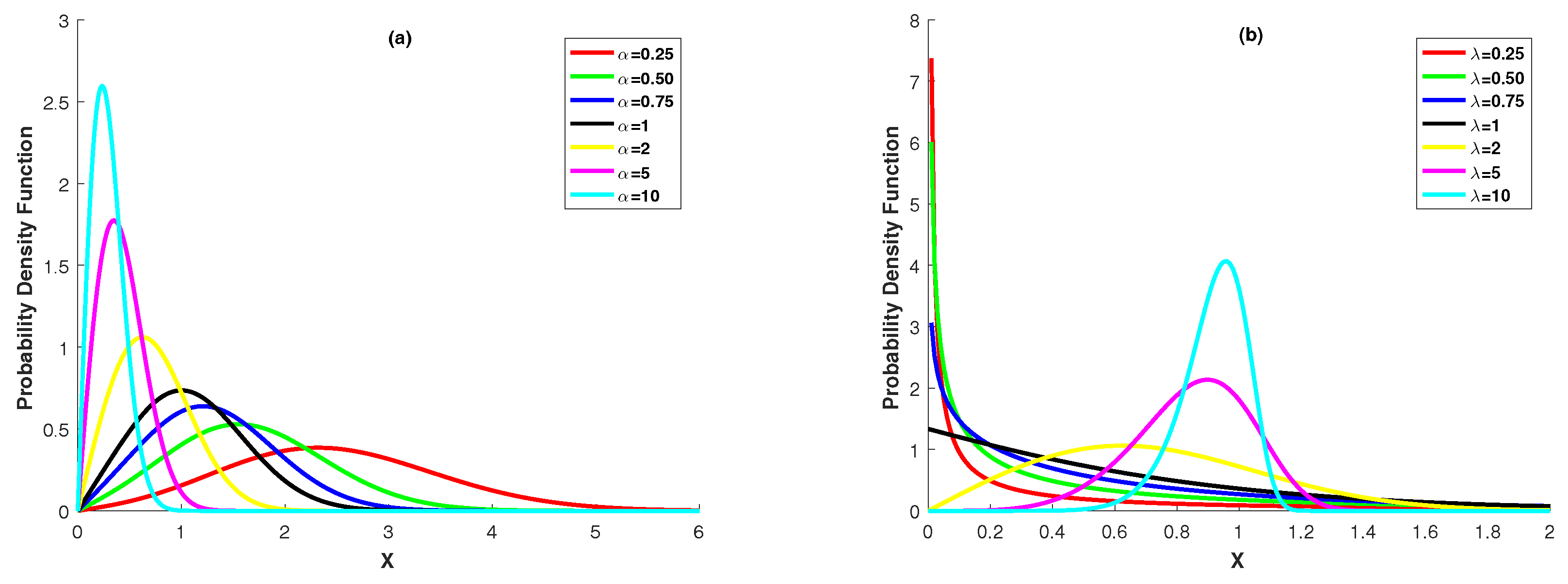
. The Power Lindley distribution is a quite important alternative to standard distribution families for analyzing of lifetime data, since its distribution function, survival function and hazard function are expressed in explicit form. The Power Lindley distribution also has uni-mode and belongs to the exponential family. To clearly show the shape of the distribution, we present Figure 1. Figure 1a,b show the behavior of the pdf of Power Lindley distribution at the different values of the parameters α and λ .
Some basic measures of the Power Lindley distribution are tabulated in Table 2.
Advanced readers can refer to [11] for more information on the Power Lindley distribution.

2.1. Shannon and Rényi Entropy of the Power Lindley Distribution

The entropy is a measure of variation or uncertainty of a random variable. In this subsection, we investigate the Shannon and Rényi entropy, which are the two most popular entropies for Power Lindley distribution. The Shannon entropy (SE) of a random variable X with pdf f is defined as, see [21],
H X = E l n f ( x ) .
Then, by using the pdf (4), the SE of the Power Lindley distribution is found as
H X = E ln f x , α , λ = 0 ln α λ 2 1 + λ + α 1 ln x λ x α f x , α , λ d x = ln α λ 2 1 + λ + α 1 0 ln x f x , α , λ d x λ 0 x α f x , α , λ d x = ln α λ 2 1 + λ + α 1 E ln X λ E X α = ln α λ 2 1 + λ + α 1 E ln X λ E X α = λ α α λ + 1 + α α 2 λ + 1 α 1 1 1 + λ Ψ 1 + ln λ α 1 + λ ln α λ 2 1 + λ ,
where Ψ . is the digamma function [22]. The Rényi entropy of a random variable with pdf f is defined as
R E X ξ = 1 1 ξ log f x ξ d x .
By using the pdf (4), Rényi entropy of the Power Lindley distribution is obtained as follows:
R E X ξ = 1 1 ξ log α λ 2 1 + λ 1 + x α x α 1 e λ x α ξ d x = 1 1 ξ log α λ 2 1 + λ ξ x α 1 e λ x α ξ 1 + x α ξ d x .
Applying the power expansion formula and gamma function to Equation (9), R E X ξ is obtained as
R E X ξ = 1 1 ξ log α λ 2 1 + λ ξ i = 0 ξ ξ i x α 1 e λ x α ξ x ξ α d x = 1 1 ξ log α λ 2 1 + λ ξ i = 0 ξ ξ i ( λ ξ ) 2 α ξ + ξ 1 α Γ 2 α ξ ξ + 1 α α .

3. Estimation of Parameters of GP with Power Lindley Distribution

3.1. Maximum Likelihood Estimation

Let X 1 , X 2 , , X n be a random sample from a GP with ratio a and X 1 P L α , λ . The likelihood function for X i , i = 1 , 2 , , n is
L ( a , α , λ ) = a n n 1 2 α n λ 2 n λ + 1 n i = 1 n 1 + a i 1 x i α a i 1 x i α 1 e λ a i 1 x i α .
From Equation (11), the corresponding log-likelihood function can be written as below:
ln L ( a , α , λ ) = n n 1 2 ln a + n ln α + 2 ln λ ln λ + 1 + i = 1 n ln 1 + a i 1 x i α + α 1 j = 1 n ln a j 1 x j λ i = 1 n a i 1 x i α .
If the first derivatives of Equation (12) with respect to a , α and λ are taken, we have the following likelihood equations:
ln L ( a , α , λ ) a = α n n 1 2 a + α i = 1 n a i 2 a i 1 x i α 1 a i 1 x i α + 1 x i i 1 λ i = 1 n α a i 1 x i α 1 x i i 1 a i 2 = 0 ,
ln L ( a , α , λ ) α = n α + i = 1 n ln a i 1 x i a i 1 x i α a i 1 x i α + 1 + i = 1 n ln a i 1 x i λ i = 1 n ln 1 a a i x i 1 a a i x i α = 0
and
ln L ( a , α , λ ) λ = 2 n λ + n λ + 1 i = 1 n a i 1 x i α = 0 .
From the solution of likelihood Equations (13)–(15), the parameter λ is obtained as
λ a ^ , α ^ = 1 X ¯ a α + 6 X ¯ a α + X ¯ a α 2 + 1 2 X ¯ a α ,
where X ¯ a α = i = 1 n a ^ i 1 x i α ^ n . However, analytical expressions for the ML estimators of the parameters a and α cannot be obtained from likelihood Equations (13)–(15). In order to estimate these parameters, Equations (13)–(15) must be simultaneously solved by using a numerical method such as Newton’s method.
Let θ = a α λ be the parameter vector and θ corresponding gradient vector for this parameter vector, i.e.,
θ = ln L ( a , λ ) a ln L ( a , λ ) α ln L ( a , λ ) λ .
Under these notations, Newton’s method is given as
θ m + 1 = θ m H 1 θ m θ m ,
where m is the iteration number and H 1 θ is the inverse of the Hessian matrix H θ , H θ R 3 × 3 . The elements of the matrix H θ are of the second derivatives of the log-likelihood function given in Equation (11) with respect to parameters a , α and λ . Let h i j be the i , j t h i , j = 1 , 2 , 3 element of the matrix H θ . The h i j s are obtained as below:
h 11 = 2 ln L a 2 = α n n 1 2 a 2 + α i = 1 n 1 a 2 a i 1 x i α a i 1 x i α + 1 2 i 1 α i α + a i 1 x i α + 1 λ i = 1 n 1 a 2 α a i 1 x i α i 1 α i α + 1 ,
h 12 = 2 ln L a α = n n 1 2 a + i = 1 n a i 1 x i α a + a a i 1 x i α i 1 + α i = 1 n 1 a ln a i 1 x i a i 1 x i α a i 1 x i α + 1 2 i 1 λ i = 1 n a i 2 a i 1 x i α 1 α ln a i 1 x i + 1 x i i 1 ,
h 13 = 2 ln L a λ = α i = 1 n a i 1 x i α 1 x i i 1 a i 2 ,
h 21 = 2 ln L α a = n n 1 2 a + 1 a i = 1 n a i 1 x i α a i 1 x i α + 1 2 i 1 α ln a i 1 x i + a i 1 x i α + 1 λ i = 1 n 1 a a i 1 x i α α ln a i 1 x i + 1 i 1 ,
h 22 = 2 ln L α 2 = n α 2 + i = 1 n ln a i 1 x i 2 a i 1 x i α a i 1 x i α + 1 2 λ i = 1 n ln a i 1 x i 2 a i 1 x i α ,
h 23 = 2 ln L α λ = i = 1 n ln a i 1 x i a i 1 x i α ,
h 31 = 2 ln L λ a = α i = 1 n a i 1 x i α 1 x i i 1 a i 2 ,
h 32 = 2 ln L λ a = i = 1 n ln a i 1 x i a i 1 x i α ,
h 33 = 2 ln L λ 2 = 2 n λ 2 n λ + 1 2 .
Hence, H 1 θ is obtained as
H 1 θ = 1 D e t H θ h 22 h 33 h 23 h 32 h 12 h 33 h 13 h 32 h 12 h 23 h 13 h 22 h 21 h 33 h 31 h 23 h 11 h 33 h 13 h 31 h 11 h 23 h 21 h 13 h 21 h 32 h 22 h 31 h 11 h 32 h 12 h 31 h 11 h 22 h 12 h 21 ,
where D e t H θ is the determinant of the matrice H θ and it is calculated by
D e t H θ = h 11 h 22 h 33 h 11 h 23 h 32 h 12 h 21 h 33 + h 12 h 31 h 23 + h 21 h 13 h 32 h 13 h 22 h 31 .
Thus, by starting with being given an initial estimation θ 0 , the parameter vector θ can be estimated with an iterative method given by (18). Hence, the ML estimates of the parameters a , α and λ , say a ^ M L , α ^ M L and λ ^ M L , respectively, are obtained as respective elements of the θ m . The joint distribution of a ^ M L , a ^ M L and a ^ M L estimators is asymptotically normal with mean vector a , α , λ and covariance matrix I 1 a , α , λ , (see, [23]), where I is the Fisher information matrix, i.e.,
I = E ln L ( a , α , λ ) a 2 E ln L ( a , α , λ ) a α E ln L ( a , α , λ ) a λ E ln L ( a , λ ) α a E ln L ( a , α , λ ) α 2 E ln L ( a , α , λ ) a λ E ln L ( a , λ ) λ a E ln L ( a , α , λ ) λ α E ln L ( a , α , λ ) λ 2 .
The elements of the Fisher information matrix I given by (21) are immediately written from elements of the Hessian matrix H θ . However, an explicit form of the Fisher information matrix I cannot be derived. Fortunately, as an estimator, the observed information matrix can be used instead of matrix I. Note that the observed information matrix of the estimators is the negative value of the matrix H θ obtained at the last iteration.

3.2. Modified Methods

Since GP is a monotonic stochastic process, some divergence problems may arise in the estimation stage of the ratio parameter a. To overcome this problem, estimating the ratio parameter a by nonparametrically is a widely used method in statistical inference for GP [2,24]. A nonparametric estimator for the ratio parameter a is given by, see [6,25],
a ^ N P = exp 6 n 1 n n + 1 i = 1 n n 2 i + 1 ln X i .
The estimator a ^ N P is an unbiased estimator and follows the asymptotic normal distribution, see [25]. When the a ^ N P given by (22) is substituted into Equation (1), it can be immediately written
Y ^ i = a ^ N P i 1 X i , i = 1 , 2 , , n .
Thus, the parameters α and λ can be estimated with a selected estimation method by using the estimators Y ^ i i = 1 , 2 , , n . This estimation rule is called modified method (see [6]).

3.2.1. MM Estimation

Let X 1 , X 2 , , X n be a random sample from a GP with ratio a and X 1 P L ( α , λ ) . In addition, we assume that the ratio parameter a is nonparametrically estimated by (22). For the sample X 1 , X 2 , , X n , first and second sample moments, m 1 and m 2 , are calculated by
m 1 = 1 n i = 1 n a ^ N P i 1 X i
and
m 2 = 1 n i = 1 n a ^ N P 2 i 1 X i 2 ,
respectively. On the other hand, from Table 2, first and second population moments of the distribution P L ( α , λ ) , say μ 1 and μ 2 , can be easily written as
μ 1 = Γ 1 α α λ + 1 + 1 α 2 λ 1 / α λ + 1
and
μ 2 = 2 Γ 2 α α λ + 1 + 2 α 2 λ 2 / α λ + 1 ,
respectively. Thus, the MM estimators of the parameters α and λ , α ^ M M and λ ^ M M , respectively, can be obtained from the solution of the following nonlinear equation system:
Γ 1 α α λ + 1 + 1 α 2 λ 1 / α λ + 1 m 1 = 0 2 Γ 2 α α λ + 1 + 2 α 2 λ 2 / α λ + 1 m 2 = 0

3.2.2. MLM Estimation

In this subsection, the MLM estimators α ^ M L M and λ ^ M L M are obtained for the parameters α and λ , respectively, when the ratio parameter a is estimated by (22). L-moments’ estimators have been proposed as a method based on the linear combination of the order statistics by Hosking [26]. Due to their useful and robust structure, the L-moments estimators have been intensively studied and, in order to estimate the unknown parameters of many probability distributions, L-moment estimators have been obtained. For more information about the L-moments, we refer the readers to [26].
As in the method of moments, to obtain the L-moment estimators, population L-moments are equated to sample L-moments. In our problem, the first two samples and population L-moments are necessary for obtaining the estimators α ^ M L M and λ ^ M L M . Under the transform Y ^ i = a ^ i 1 X i , i = 1 , , n , first and second sample L-moments are calculated as follows, see [26]:
l 1 = 1 n i = 1 n Y ^ ( i ) ,
l 2 = 2 n n 1 i = 1 n i 1 Y ^ ( i ) l 1 ,
where Y ^ ( i ) , i = 1 , 2 , , n represents the ordered observations. On the other hand, using the notations in [26], first and second population L-moments of P L λ , α are
L 1 = λ λ + 1 Γ 1 α + 1 λ 1 α + 1 λ + 1 Γ 1 α + 2 λ 1 α = Γ 1 α α + α λ + 1 α 2 λ 1 α λ + 1
and
L 2 = Γ 1 α α λ + 1 + 1 α 2 λ 1 α λ + 1 2 α λ 2 1 + λ Γ α + 1 α α 2 λ α + 1 α + Γ 2 α + 1 α α 2 λ 2 α + 1 α 2 α λ 3 1 + λ 2 Γ 2 α + 1 α α 2 λ 2 α + 1 α + Γ 3 α + 1 α α 2 λ 3 α + 1 α .
See Appendix A for the derivation of population L-moments.
Thus, the estimators α ^ M L M and λ ^ M L M are obtained from the numerical solution of the following nonlinear system:
Γ 1 α α + α λ + 1 α 2 λ 1 α λ + 1 l 1 = 0 , Γ 1 α α λ + 1 + 1 α 2 λ 1 α λ + 1 2 α λ 2 1 + λ Γ α + 1 α α 2 λ α + 1 α + Γ 2 α + 1 α α 2 λ 2 α + 1 α
2 α λ 3 1 + λ 2 Γ 2 α + 1 α α 2 λ 2 α + 1 α + Γ 3 α + 1 α α 2 λ 3 α + 1 α l 2 = 0 .

3.2.3. MLS Estimation

The least-squares estimator (LSE) is a regression-based method proposed by Swain et al. [27]. Essentially, the method is a nonlinear curve fitting for the cdf of a random variable by using the empirical distribution function. In the least-squares method, the estimator(s) is determined such that the squared difference between the empirical distribution function and the fitted curve is minimum. Let Z 1 , , Z n be a random sample from a distribution function F Z ( . ) . In addition, the order statistics of the random sample Z 1 , , Z n are represented by Z ( 1 ) , , Z ( n ) . In this situation, the LSE of the parameters are obtained minimizing
j = 1 n F Z ( Z ( i ) ) E F Z ( Z ( i ) 2
with respect to the parameters of F Z ( . ) [27], where expectation E F Z ( Z ( i ) is calculated by
E F Z ( Z ( i ) = i n + 1 , i = 1 , 2 , , n .
Therefore, in our problem, the MLS estimators of parameters α and λ , say α ^ M L S and λ ^ M L S , respectively, are obtained by minimizing
j = 1 n 1 1 + λ λ + 1 Y j α e λ Y j α j n + 1 2
with respect to α and λ .

4. Simulation Study

In order to evaluate the estimation performances of the ML, the MLS, the MM and the MLM estimators obtained in the previous section, some Monte Carlo simulation experiments are presented in this section. Throughout the simulation experiments, the scale parameter λ is assumed to be 0.5 , without loss of generality and also the parameter α set as 0.5 , 1 , 1.5 and 2. For different sample size n = 30 , 50 , 100 , 150 and ratio parameter a = 0.90 , 0.95 , 1.05 , 1.10 , values of means, biases and MSEs have been calculated for estimating the ML, the MLS, the MM and the MLM. The obtained results based on 10,000 replications are displayed in Table 3, Table 4, Table 5 and Table 6.
When the results of the simulation experiments given in Table 3, Table 4, Table 5 and Table 6 are analyzed, it is seen that the ML estimators have smaller MSE values than the other estimators in all cases. Therefore, the ML estimators outperform the modified estimators with smaller bias and MSE. In addition, when the sample size n increases, the values of the bias and MSE decrease for all estimators. Based on this result, it can be said that all estimators obtained in the previous section are asymptotically unbiased and consistent.

5. Illustrative Examples

Practical applications of the parameter estimation with developed procedures in Section 3 are illustrated in this section with two data sets called Aircraft data set and Coal mining disaster data set.
In the examples, we use two criteria, the mean-squared error (MSE*) [28] for the fitted values and the maximum percentage error (MPE), which are defined in [25], for comparing the stochastic processes GP and RP. The MSE* and MPE are described as follows:
  • MSE* = 1 / n k = 1 n X k X ^ k 2 ,
  • MPE = max 1 k n S k S ^ k / S k ,
where X ^ k is calculated by
X ^ k = μ ^ M L a ^ M L 1 k GP with the ML estimators , μ ^ M L S a ^ M L S 1 k GP with the MLS estimators , μ ^ M M a ^ M M 1 k GP with the MM estimators , μ ^ M L M a ^ M L M 1 k GP with the MLM estimators , μ ^ M L RP with the MLestimators ,
and S k = X 1 + X 2 + + X k , k = 1 , 2 , , n and S ^ k = j = 1 k X ^ j . Then, in order to compare the relative performances of the RP and four GPs with the ML, the MLS, the MM and the MLM estimators, the plot of S k and S ^ k against k , k = 1 , 2 , , n can be used.
Example 1.
Aircraft data.
The aircraft dataset consists of 30 observations that deal with the air-conditioning system failure times of a Boeing 720 aircraft (aircraft number 7912). The aircraft dataset was originally studied by Proschan [29]. The successive failure times in aircraft dataset are 23, 261, 87, 7, 120, 14, 62, 47, 225, 71, 246, 21, 42, 20, 5, 12, 120, 11, 3, 14, 71, 11, 14, 11, 16, 90, 1, 16, 52, 95.
We first investigate the underlying distribution of the set of data. To test whether the underlying distribution of the data { X 1 , , X n } is the Power Lindley, the following procedures can be used. From Definition 1, we know that the Y i = a i 1 X i and the Y i s follow the Power Lindley. We can write immediately as ln Y i = i 1 ln a + ln X i by taking the logarithm of Y i . Note that ln Y i s follow the Log-Power Lindley distribution. Therefore, a linear regression model
ln X i = μ i 1 ln a + ε i
can be defined, where μ = E ln Y i and exp ( ε i ) P L θ , β . If the exponential errors are Power Lindley distributed, then the underlying distribution of the set of data is Power Lindley. The error term ε i in Equation (39) can be estimated by
ε ^ i = ln X i μ ^ i 1 ln a ^ N L ,
where μ ^ = n n 1 2 ln a ^ N L + i = 1 n ln X i 
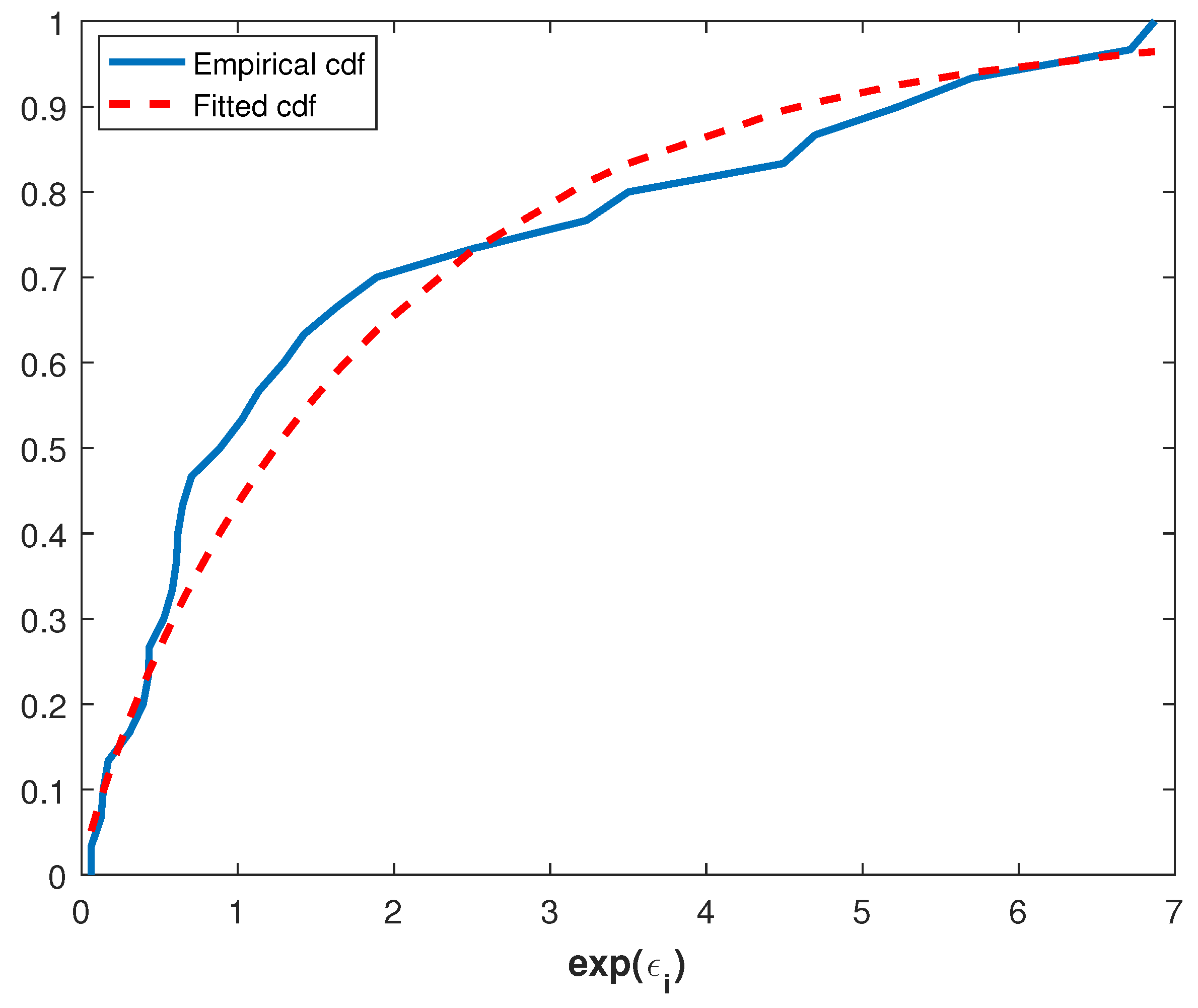
. Thus, consistency of the exponentiated errors to Power Lindley distribution can be tested by using a goodness of fit test such as Kolmogorov–Smirnov (K-S). The parameter estimates of the exponentiated errors are θ = 0.9717 and β = 0.7985 and also the value of the K-S test is 0.1225 and the corresponding p-value is 0.7134. Therefore, it can be said that the underlying distribution of this data set is Power Lindley. This can also be seen from Figure 2, which illustrates the plots of the empirical and the fitted cdf.
When a GP with the Power Lindley distribution is used for modeling of this dataset, the ML, the MLS, the MM and the MLM estimates of the parameters a , α and λ and also MSE* and MPE values are tabulated in Table 3.
As it can be seen from Table 7, the ML estimates have the smallest MSE * values consistent with the simulation experiments. The estimator having the smallest MPE is the MM, but estimators of the ML and the MLM are very close to the MM.
Now, we check the model optimality. In order to select an optimal model to a data set, Akaike information criterion (AIC) and maximized log-likelihood (L) value are commonly used methods. For deciding an optimal model among the Power Lindley and its alternatives (Log-Normal, Gamma and inverse Gaussian) for this data set, we compute the -L and AIC values. The -L and AIC values for the models are given in Table 8.
The results given in 
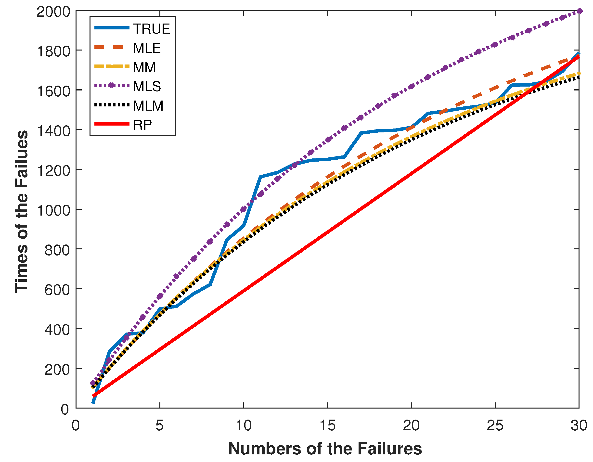
Table 8 show that the Power Lindley distribution is an optimal model for the aircraft dataset with smaller AIC and -L values. In Figure 3, the failure times for the aircraft data and their fitted times are plotted.
The modeling performances of the RP and GP with the ML, the MLS, the MM and the MLM estimators can be easily compared by Figure 3. By Figure 3, the GP with the ML, the MLS, the MM and the MLM estimators outperform the RP. This result is compatible with Table 7.
Example 2.
Coal mining disaster data.
This example is from [30] on the intervals in days between successive disasters in Great Britain from 1851 to 1962. The coal mining disaster data set, which includes 190 successive intervals, was used as an illustrative example for GP by [7,10,24].
For this data set, the value of K-S test is 0.0396 and the corresponding p-value is 0.9148. Thus, the Power Lindley distribution is an appropriate model for the coal mining disaster data. This is also supported by the following Q-Q plot, Figure 4, which is constructed by plotting the ordered exponential errors exp ε ^ i against the quantiles of the P L ( 0.9552 , 0.7930 ) because the data points fall approximately on the straight line in Figure 4.
For the coal mining disaster data set, the estimates of the parameters a, λ and α are given in Table 9.
Moreover, calculated AIC and L values for the coal mining disaster data set with the different models are tabulated in Table 10.
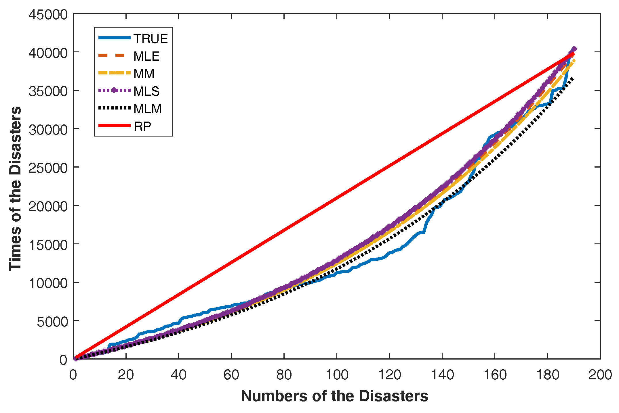
We can say that the Power Lindley distribution is an optimal model for this data set since it has minimum AIC and -L values. Under the assumption that the underlying distribution of the data is Power Lindley, we present Figure 5 for comparing the modeling performance of the RP and the GP with four estimators obtained in the previous section. Figure 5 plots S k and S ^ k versus the number of disasters k , k = 1 , 2 , , n .
As can be seen in Figure 5, the GP with the ML, the MLS, the MM and the MLM estimators more fairly follow real values than the RP. It can also be seen from Table 9 that the MSE* and MPE values of GP models are much smaller than RP. Thus, according to Figure 5 and Table 9, it is concluded that the GP provides the better data fit than RP.

6. Conclusions

In this paper, we have discussed the parameter estimation problem for GP by assuming that distribution of the first inter-arrival time is Power Lindley with parameters α and λ . In the paper, the parameter estimation problem has been solved from two points of view as the parametric (ML) and nonparametric (MLS, MM and MLM). Parametric estimators, ML, of the parameters A, ALF and LAM are also asymptotically normally distributed. However, more work should be done in order to say something about the asymptotic properties of nonparametric estimators MLS, MM and MLM. In addition, this is usually not an easy task because an analytical form of these estimators cannot be written.
Numerical study results have shown that the ML estimators outperform the MLS, MLM and MLS estimators with smaller bias and MSE measures. In addition, it has been observed that both bias and MSE values of all estimators decrease when the sample size increases. Hence, in light of numerical studies, it can be concluded that all of the estimators are asymptotically unbiased and consistent.
In the illustrative examples presented to demonstrate the data modeling performance of GP with the obtained estimators, the GP with Power Lindley distribution gives a better data fit than the RP in both examples. In addition, according to AIC and -L values, it can be said that modeling both the aircraft dataset and the coal mining disaster dataset using a GP with Power Lindley distribution is more appropriate than a GP with Gamma, log-normal or inverse Gaussian distribution. Therefore, it can be said that a GP with Power Lindley distribution is a quite important alternative to a GP with famous distributions such as Gamma, Log-normal or inverse Gaussian in modeling the successive inter-arrival times.

Funding

This research received no external funding

Acknowledgments

The author is sincerely grateful to the anonymous referees for their comments and suggestions that greatly improved an early version of this paper.

Conflicts of Interest

The authors declare no conflict of interest.

Appendix A

According to [26], the first two population L-moments of a continuous distribution are calculated by
L 1 = x f x d x
and
L 2 = x 2 F x 1 f x d x ,
respectively, where f x and F x are the pdf and the cdf of the random variable X. Obviously, the first popuplation L-moment L 1 is the expectation of random variable X . Thus, from Table 2, the first L-moment of Power Lindley distribution is
L 1 = Γ 1 α α λ + 1 + 1 α 2 λ 1 / α λ + 1 .
Now, we calculate the second population L-moment of Power Lindley distribution. Substituting the cdf given by (5) into (A2), we can write
L 2 = 0 x 2 1 1 + λ λ + 1 x α e λ x α 1 f ( x ) d x = 0 x 2 1 1 + λ λ + 1 x α e λ x α 1 f ( x ) d x = 0 2 x 1 1 + λ λ + 1 x α e λ x α x f ( x ) d x = 0 2 x 1 1 + λ λ + 1 x α e λ x α f ( x ) d x 0 x f ( x ) d x = 0 2 x f ( x ) d x 0 2 x 1 + λ λ + 1 x α e λ x α f ( x ) d x 0 x f ( x ) d x = 0 x f ( x ) d x 0 2 x 1 + λ λ + 1 x α e λ x α f ( x ) d x = 0 x f ( x ) d x 0 2 x λ + 1 + λ x α λ + 1 e λ x α f ( x ) d x = E X 0 2 x λ + 1 + λ x α λ + 1 e λ x α f ( x ) d x = Γ 1 α α λ + 1 + 1 α 2 λ 1 / α λ + 1 0 2 x 1 + λ x α λ + 1 e λ x α f ( x ) d x = Γ 1 α α λ + 1 + 1 α 2 λ 1 / α λ + 1 0 2 x e λ x α f ( x ) d x 0 2 λ x α + 1 λ + 1 e λ x α f ( x ) d x .
In the last equality, using f x given in (4), it can be easily written
L 2 = Γ 1 α α λ + 1 + 1 α 2 λ 1 / α λ + 1 0 2 x e λ x α α λ 2 1 + λ 1 + x α x α 1 e λ x α d x 0 2 λ x α + 1 λ + 1 e λ x α α λ 2 1 + λ 1 + x α x α 1 e λ x α d x = Γ 1 α α λ + 1 + 1 α 2 λ 1 / α λ + 1 2 0 α λ 2 1 + λ 1 + x α x α e 2 λ x α d x 2 λ 1 + λ 0 α λ 2 1 + λ 1 + x α x 2 α e 2 λ x α d x = Γ 1 α α λ + 1 + 1 α 2 λ 1 / α λ + 1 2 α λ 2 1 + λ 0 x α + x 2 α e 2 λ x α d x 2 α λ 3 1 + λ 2 0 x 2 α + x 3 α e 2 λ x α d x = Γ 1 α α λ + 1 + 1 α 2 λ 1 / α λ + 1 2 α λ 2 1 + λ 0 x α e 2 λ x α d x + 0 x 2 α e 2 λ x α d x 2 α λ 3 1 + λ 2 0 x 2 α e 2 λ x α d x + 0 x 3 α e 2 λ x α d x .
Therefore, by using the gamma function, we have
L 2 = Γ 1 α α λ + 1 + 1 α 2 λ 1 α λ + 1 2 α λ 2 1 + λ Γ α + 1 α α 2 λ α + 1 α + Γ 2 α + 1 α α 2 λ 2 α + 1 α 2 α λ 3 1 + λ 2 Γ 2 α + 1 α α 2 λ 2 α + 1 α + Γ 3 α + 1 α α 2 λ 3 α + 1 α .

References

  1. Lam, Y. Geometric processes and replacement problem. Acta Math. Appl. Sin. 1988, 4, 366–377. [Google Scholar]
  2. Lam, Y. The Geometric Process and Its Applications; World Scientific: Singapore, 2007. [Google Scholar]
  3. Demirci Bicer, H.; Bicer, C. Discrimination Between Gamma and Lognormal Distributions for Geometric Process Data. In Researches on Science and Art in 21st Century Turkey; Gece Publishing: Ankara, Turkey, 2017; Chapter 315; pp. 2830–2836. [Google Scholar]
  4. Demirci Bicer, H.; Bicer, C. Discriminating between the Gamma and Weibull Distributions for Geometric Process Data. Int. J. Econ. Admin. Stud. 2018, 18, 239–252. [Google Scholar] [CrossRef]
  5. Chan, J.S.; Lam, Y.; Leung, D.Y. Statistical inference for geometric processes with gamma distributions. Comput. Stat. Data Anal. 2004, 47, 565–581. [Google Scholar] [CrossRef]
  6. Lam, Y.; Chan, S.K. Statistical inference for geometric processes with lognormal distribution. Comput. Stat. Data Anal. 1998, 27, 99–112. [Google Scholar] [CrossRef]
  7. Kara, M.; Aydogdu, H.; Turksen, O. Statistical inference for geometric process with the inverse Gaussian distribution. J. Stat. Comput. Simul. 2015, 85, 3206–3215. [Google Scholar] [CrossRef]
  8. Biçer, C.; Biçer, H.D.; Kara, M.; Aydoğdu, H. Statistical inference for geometric process with the Rayleigh distribution. Commun. Fac. Sci. Univ. Ankara Ser. A1 Math. Stat. 2019, 68, 149–160. [Google Scholar]
  9. Bicer, C. Statistical Inference for Geometric Process with the Two-parameter Rayleigh Distribution. In The Most Recent Studies in Science and Art; Gece Publishing: Ankara, Turkey, 2018; Chapter 43; pp. 576–583. [Google Scholar]
  10. Bicer, C.; Demirci Bicer, H. Statistical Inference for Geometric Process with the Lindley Distribution. In Researches on Science and Art in 21st Century Turkey; Gece Publishing: Ankara, Turkey, 2017; Chapter 314; pp. 2821–2829. [Google Scholar]
  11. Ghitany, M.; Al-Mutairi, D.K.; Balakrishnan, N.; Al-Enezi, L. Power Lindley distribution and associated inference. Comput. Stat. Data Anal. 2013, 64, 20–33. [Google Scholar] [CrossRef]
  12. Pararai, M.; Warahena-Liyanage, G.; Oluyede, B.O. Exponentiated power Lindley–Poisson distribution: Properties and applications. Commun. Stat. Theory Methods 2017, 46, 4726–4755. [Google Scholar] [CrossRef]
  13. Ashour, S.K.; Eltehiwy, M.A. Exponentiated power Lindley distribution. J. Adv. Res. 2015, 6, 895–905. [Google Scholar] [CrossRef] [PubMed]
  14. Alizadeh, M.; MirMostafaee, S.; Ghosh, I. A new extension of power Lindley distribution for analyzing bimodal data. Chil. J. Stat. 2017, 8, 67–86. [Google Scholar]
  15. Warahena-Liyanage, G.; Pararai, M. A generalized power Lindley distribution with applications. Asian J. Math. Appl. 2014, 2014, ama0169. [Google Scholar]
  16. Alizadeh, M.; Altun, E.; Ozel, G. Odd Burr power Lindley distribution with properties and applications. Gazi Univ. J. Sci. 2017, 30, 139–159. [Google Scholar]
  17. Iriarte, Y.A.; Rojas, M.A. Slashed power-Lindley distribution. Commun. Stat. Theory Methods 2018, 1–12. [Google Scholar] [CrossRef]
  18. Barco, K.V.P.; Mazucheli, J.; Janeiro, V. The inverse power Lindley distribution. Commun. Stat. Simul. Comput. 2017, 46, 6308–6323. [Google Scholar] [CrossRef]
  19. Alizadeh, M.; K MirMostafaee, S.; Altun, E.; Ozel, G.; Khan Ahmadi, M. The odd log-logistic Marshall-Olkin power Lindley Distribution: Properties and applications. J. Stat. Manag. Syst. 2017, 20, 1065–1093. [Google Scholar] [CrossRef]
  20. Demirci Bicer, H. Parameter Estimation for Finite Mixtures of Power Lindley Distributions. In The Most Recent Studies in Science and Art; Gece Publishing: Ankara, Turkey, 2018; Chapter 128; pp. 1659–1669. [Google Scholar]
  21. Arellano-Valle, R.B.; Contreras-Reyes, J.E.; Stehlík, M. Generalized skew-normal negentropy and its application to fish condition factor time series. Entropy 2017, 19, 528. [Google Scholar] [CrossRef]
  22. Abramowitz, M.; Stegun, I.A. Handbook of Mathematical Functions: With Formulas, Graphs, and Mathematical Tables; Courier Corporation: Chelmsford, MA, USA, 1964; Volume 55. [Google Scholar]
  23. Cox, D.; Barndorff-Nielsen, O. Inference and Asymptotics; CRC Press: Boca Raton, FL, USA, 1994. [Google Scholar]
  24. Yeh, L. Nonparametric inference for geometric processes. Commun. Stat. Theory Methods 1992, 21, 2083–2105. [Google Scholar] [CrossRef]
  25. Lam, Y.; Zhu, L.X.; Chan, J.S.; Liu, Q. Analysis of data from a series of events by a geometric process model. Acta Math. Appl. Sin. Engl. Ser. 2004, 20, 263–282. [Google Scholar] [CrossRef]
  26. Hosking, J.R. L-moments: Analysis and estimation of distributions using linear combinations of order statistics. J. R. Stat. Soc. Ser. B (Methodol.) 1990, 52, 105–124. [Google Scholar]
  27. Swain, J.J.; Venkatraman, S.; Wilson, J.R. Least-squares estimation of distribution functions in Johnson’s translation system. J. Stat. Comput. Simul. 1988, 29, 271–297. [Google Scholar] [CrossRef]
  28. Wand, M.; Jones, M. Kernel Smoothing; Chapman & Hall: London, UK, 1995. [Google Scholar]
  29. Proschan, F. Theoretical explanation of observed decreasing failure rate. Technometrics 1963, 5, 375–383. [Google Scholar] [CrossRef]
  30. Andrews, D.; Herzberg, A. Data; Springer: New York, NY, USA, 1985. [Google Scholar]
Figure 1. Pdf of the Power Lindley distribution (a): α = 0.25 , 0.50 , 0.75 , 1 , 2 , 5 , 10 and λ = 2 ; (b) α = 2 and λ = 0.25 , 0.50 , 0.75 , 1 , 2 , 5 , 10 .
Entropy 20 00723 g001
Figure 2. Empirical and fitted cdf of the exp ( ε ^ i ) .
Entropy 20 00723 g002
Figure 3. The plots of S k and S ^ k against the number of failures for the aircraft data.
Entropy 20 00723 g003
Figure 4. Q-Q plot of the coal mining disaster data.
Entropy 20 00723 g004
Figure 5. The plots S k and S ^ k against the number of failures for the coal mining disaster data.
Entropy 20 00723 g005
Table 1. Behavior of GP according to values of ratio parameter a.
Value of Parameter aBehavior of GP
a > 1Stochastically decreasing process
a < 1Stochastically increasing process
a = 1Stable (GP is an RP)
Table 2. Some basic measures of the Power Lindley distributions.
CharacteristicValue
Expectation ( μ ) Γ 1 α α λ + 1 + 1 α 2 λ 1 / α λ + 1
kth moment ( μ k ) k Γ k α α λ + 1 + k α 2 λ k / α λ + 1
Variance ( σ 2 ) 2 Γ 2 α α λ + 1 + 2 α 2 λ + 1 Γ 1 α 2 α λ + 1 + 1 2 α 4 λ 2 / α λ + 1 2
Kurtosis μ 4 4 μ 3 μ + 6 μ 2 μ 2 3 μ 4 σ 4
Skewness μ 3 3 μ 2 μ + 2 μ 3 σ 3
Table 3. The simulated Means, Biases and n × MSE values for the MLE, MLS, MM and MLM estimators of the parameters a, α and λ , when α = 0.5 .
a ^ λ ^ α ^
anMethodMeanBiasn × MSEMeanBiasn × MSEMeanBiasn × MSE
0.9030MLE0.90020.00020.52730.50500.005012.84200.52830.02832.8920
MLS0.90060.00060.88380.54610.046120.18920.4977−0.00233.3405
MM0.90060.00060.88380.4657−0.034320.34220.56390.06396.6133
MLM0.90060.00060.88380.63820.138239.26760.4634−0.03663.7622
50MLE0.90020.00020.12270.50480.00487.44170.51720.01721.4622
MLS0.8994−0.00060.21860.53420.034212.45240.50180.00181.9141
MM0.8994−0.00060.21860.4877−0.012315.36390.53970.03973.8289
MLM0.8994−0.00060.21860.63020.130226.51010.4585−0.04152.6689
100MLE0.90020.00020.01260.4948−0.00523.34530.50970.00970.7602
MLS0.90010.00010.02190.50730.00734.89250.50220.00220.9723
MM0.90010.00010.02190.4730−0.02707.34050.52960.02962.2908
MLM0.90010.00010.02190.59220.092211.40400.4610−0.03901.7020
150MLE0.8998−0.00020.00370.50100.00102.15600.50710.00710.4934
MLS0.90000.00000.00620.50570.00572.96260.50050.00050.6753
MM0.90000.00000.00620.4774−0.02265.32860.52350.02351.5998
MLM0.90000.00000.00620.58530.08538.03500.4617−0.03831.3375
0.9530MLE0.95220.00220.63060.4870−0.013013.15260.53280.03282.9722
MLS0.95280.00281.06150.52350.023519.09080.50380.00383.0317
MM0.95280.00281.06150.4519−0.048120.74070.56670.06677.1428
MLM0.95280.00281.06150.61770.117735.08480.4675−0.03253.8529
50MLE0.9493−0.00070.10610.4989−0.00116.73880.51850.01851.6173
MLS0.9495−0.00050.18210.52100.02109.62920.50040.00041.8929
MM0.9495−0.00050.18210.4678−0.032212.64750.54490.04494.2641
MLM0.9495−0.00050.18210.60930.109320.95500.4624−0.03762.6568
100MLE0.9497−0.00030.01620.50600.00603.50160.50920.00920.7257
MLS0.9499−0.00010.02450.51550.01554.75810.4999−0.00010.9493
MM0.9499−0.00010.02450.4854−0.01468.08050.52620.02622.3448
MLM0.9499−0.00010.02450.60000.100012.53840.4604−0.03961.7649
150MLE0.9498−0.00020.00470.50060.00062.29890.50700.00700.4819
MLS0.9497−0.00030.00800.50860.00863.13560.50260.00260.6549
MM0.9497−0.00030.00800.4903−0.00975.69510.51860.01861.5909
MLM0.9497−0.00030.00800.59340.09349.19330.4603−0.03971.4338
1.0530MLE1.05010.00010.66030.4976−0.00249.68640.52950.02952.7535
MLS1.0480−0.00201.14540.54350.043519.04800.50200.00202.9153
MM1.0480−0.00201.14540.4727−0.027319.66060.56180.06186.7118
MLM1.0480−0.00201.14540.64490.144937.99740.4613−0.03873.7214
50MLE1.0499−0.00010.15060.4998−0.00027.20300.52060.02061.7516
MLS1.05000.00000.24610.52220.022210.35390.50370.00372.1801
MM1.05000.00000.24610.4748−0.025213.44120.54360.04364.1555
MLM1.05000.00000.24610.61220.112221.45270.4630−0.03702.5071
100MLE1.05040.00040.01900.4930−0.00703.48840.50970.00970.6671
MLS1.05060.00060.03140.50250.00254.39820.50060.00060.9108
MM1.05060.00060.03140.4715−0.02858.08950.52740.02742.1731
MLM1.05060.00060.03140.58420.084210.69680.4617−0.03831.5892
150MLE1.05000.00000.00560.4949−0.00512.09590.50820.00820.4612
MLS1.0499−0.00010.01070.50530.00533.26640.50300.00300.6055
MM1.0499−0.00010.01070.4889−0.01115.89120.51760.01761.6345
MLM1.0499−0.00010.01070.59090.09099.33570.4597−0.04031.4546
1.1030MLE1.10050.00050.87950.4953−0.004711.71550.53160.03162.9118
MLS1.10370.00371.48610.52560.025617.26380.50310.00313.3829
MM1.10370.00371.48610.4551−0.044919.28210.56210.06216.3725
MLM1.10370.00371.48610.62190.121934.36210.4639−0.03613.6346
50MLE1.10000.00000.16150.50590.00597.33780.51410.01411.5498
MLS1.10010.00010.27520.52970.029710.83730.4961−0.00391.8948
MM1.10010.00010.27520.4751−0.024912.91280.54070.04073.9492
MLM1.10010.00010.27520.61970.119723.36100.4582−0.04182.8084
100MLE1.0999−0.00010.01890.4974−0.00263.15630.51120.01120.7756
MLS1.0997−0.00030.03190.50950.00954.69680.50380.00380.9466
MM1.0997−0.00030.03190.4849−0.01517.80790.52560.02562.2592
MLM1.0997−0.00030.03190.59570.095712.10020.4619−0.03811.6833
150MLE1.0999−0.00010.00590.50420.00422.13810.50480.00480.4252
MLS1.0999−0.00010.01030.51150.01153.43770.4997−0.00030.6374
MM1.0999−0.00010.01030.4901−0.00996.28670.51690.01691.4973
MLM1.0999−0.00010.01030.59770.097710.13420.4566−0.04341.5425
Table 4. The simulated Means, Biases and n × MSE values for the MLE, MLS, MM and MLM estimators of the parameters a, α and λ , when α = 1 .
a ^ λ ^ α ^
anMethodMeanBiasn × MSEMeanBiasn × MSEMeanBiasn × MSE
0.9030MLE0.90100.00100.12930.4848−0.015210.05151.05780.057812.7947
MLS0.90170.00170.21930.51730.017313.91321.00210.002114.4717
MM0.90170.00170.21930.4977−0.002315.50701.04370.043714.0296
MLM0.90170.00170.21930.58210.082120.28260.9189−0.081113.4991
50MLE0.8999−0.00010.02790.4962−0.00387.44781.04200.04207.3976
MLS0.90050.00050.05190.51200.012010.15561.01020.01028.5684
MM0.90050.00050.05190.50590.005911.07081.02710.02718.1213
MLM0.90050.00050.05190.57940.079415.50750.9191−0.08099.3453
100MLE0.90000.00000.00340.4985−0.00153.69831.02070.02072.9458
MLS0.90010.00010.00600.50590.00595.28761.00570.00574.0647
MM0.90010.00010.00600.50380.00385.67391.01120.01123.5802
MLM0.90010.00010.00600.57360.07368.94710.9119−0.08816.4967
150MLE0.90000.00000.00100.4975−0.00252.11361.01430.01431.8608
MLS0.90020.00020.00170.4996−0.00042.87411.00210.00212.4144
MM0.90020.00020.00170.4999−0.00013.00321.00510.00512.5506
MLM0.90020.00020.00170.56670.06675.58420.9101−0.08995.7094
0.9530MLE0.9491−0.00090.13840.50400.004011.54941.06200.062014.5314
MLS0.9476−0.00240.23940.55330.053320.72751.00770.007716.7516
MM0.9476−0.00240.23940.53680.036820.82391.04320.043215.7827
MLM0.9476−0.00240.23940.62350.123529.91550.9161−0.083914.7327
50MLE0.95000.00000.03230.50030.00037.15571.02930.02936.0053
MLS0.95020.00020.05520.52250.022510.82950.9968−0.00328.8009
MM0.95020.00020.05520.51120.011210.92001.01860.01867.3102
MLM0.95020.00020.05520.58970.089716.13810.9064−0.09369.7342
100MLE0.9499−0.00010.00330.50020.00023.45861.01860.01863.0031
MLS0.9498−0.00020.00620.51390.01395.22831.00390.00393.6547
MM0.9498−0.00020.00620.51420.01425.48251.00710.00713.7674
MLM0.9498−0.00020.00620.58270.08279.52000.9095−0.09056.7580
150MLE0.95000.00000.00110.4996−0.00042.31511.01230.01232.0880
MLS0.95010.00010.00200.50480.00483.29181.00130.00132.7135
MM0.95010.00010.00200.50360.00363.25391.00660.00662.6992
MLM0.95010.00010.00200.57250.07256.44200.9093−0.09076.0326
1.0530MLE1.05000.00000.17120.4994−0.000614.09821.06240.062411.6667
MLS1.05100.00100.28740.53420.034222.07311.00420.004214.0411
MM1.05100.00100.28740.51300.013020.99441.04470.044712.6039
MLM1.05100.00100.28740.59890.098927.99940.9175−0.082512.5305
50MLE1.0496−0.00040.04000.50520.00527.66341.04080.04087.4367
MLS1.05020.00020.06370.52300.023010.54821.00660.00668.6068
MM1.05020.00020.06370.51460.014610.22971.02460.02468.5140
MLM1.05020.00020.06370.59100.091015.89360.9140−0.08609.6941
100MLE1.05010.00010.00480.4961−0.00393.79541.02120.02123.2199
MLS1.05000.00000.00880.51220.01225.63051.00230.00233.8942
MM1.05000.00000.00880.50750.00755.98011.01350.01353.9135
MLM1.05000.00000.00880.57840.07849.67000.9124−0.08766.6484
150MLE1.05000.00000.00130.4990−0.00102.36991.01490.01491.8542
MLS1.05010.00010.00220.50500.00503.27761.00320.00322.4563
MM1.05010.00010.00220.50220.00223.42711.00980.00982.2668
MLM1.05010.00010.00220.57200.07206.44150.9113−0.08875.5864
1.1030MLE1.0997−0.00030.19470.4944−0.005612.65681.07200.072013.7050
MLS1.0991−0.00090.31270.53460.034617.97531.01340.013416.8987
MM1.0991−0.00090.31270.51460.014618.13201.05920.059214.8263
MLM1.0991−0.00090.31270.60020.100225.54660.9303−0.069712.8303
50MLE1.10030.00030.04260.4904−0.00966.36341.04070.04076.5906
MLS1.10050.00050.07340.51350.013510.12911.00570.00578.3013
MM1.10050.00050.07340.50440.004410.06181.02530.02537.4875
MLM1.10050.00050.07340.57960.079614.72060.9160−0.08408.9003
100MLE1.10000.00000.00500.50570.00573.70031.01560.01563.1842
MLS1.10020.00020.00940.51420.01425.46400.9982−0.00184.3067
MM1.10020.00020.00940.51210.01215.57751.00540.00544.0731
MLM1.10020.00020.00940.58240.08249.65930.9063−0.09377.3535
150MLE1.0999−0.00010.00160.50400.00402.38231.01190.01191.9819
MLS1.0998−0.00020.00270.51370.01373.48261.00200.00202.6826
MM1.0998−0.00020.00270.51280.01283.68051.00620.00622.6669
MLM1.0998−0.00020.00270.58210.08217.36410.9088−0.09126.0368
Table 5. The simulated Means, Biases and n × MSE values for the MLE, MLS, MM and MLM estimators of the parameters a, α and λ , when α = 1.5 .
a ^ λ ^ α ^
anMethodMeanBiasn × MSEMeanBiasn × MSEMeanBiasn × MSE
0.9030MLE0.90050.00050.05240.50190.001911.18301.55790.057924.1329
MLS0.90060.00060.09950.53990.039918.43001.4787−0.021337.2741
MM0.90060.00060.09950.52600.026017.52071.51930.019323.9922
MLM0.90060.00060.09950.59320.093222.97961.3518−0.148232.9507
50MLE0.90010.00010.01130.50530.00536.84931.54560.045614.0863
MLS0.8999−0.00010.02180.53250.032512.13711.4997−0.000318.7168
MM0.8999−0.00010.02180.52650.026511.76921.51620.016214.6065
MLM0.8999−0.00010.02180.58650.086515.66821.3644−0.135621.2329
100MLE0.90000.00000.00140.4973−0.00273.18021.52890.02896.8488
MLS0.90010.00010.00280.50740.00744.85881.50530.005310.7571
MM0.90010.00010.00280.50920.00925.17611.50410.00417.6287
MLM0.90010.00010.00280.56400.06407.11821.3664−0.133615.2179
150MLE0.90010.00010.00040.4979−0.00212.18041.50920.00924.2275
MLS0.90010.00010.00080.50270.00273.11751.4940−0.00606.1723
MM0.90010.00010.00080.50550.00553.43951.4923−0.00775.0529
MLM0.90010.00010.00080.56090.06095.25211.3554−0.144614.3443
0.9530MLE0.9489−0.00110.06560.50820.008212.49201.59510.095128.9125
MLS0.9493−0.00070.10580.54450.044519.60361.50130.001332.1834
MM0.9493−0.00070.10580.53130.031318.84151.54610.046126.4845
MLM0.9493−0.00070.10580.59380.093823.85151.3818−0.118228.5391
50MLE0.9499−0.00010.01440.50020.00027.92141.55490.054912.8801
MLS0.95020.00020.02630.52130.021312.49341.50690.006918.9876
MM0.95020.00020.02630.51770.017712.40681.51940.019413.4693
MLM0.95020.00020.02630.57390.073915.42811.3737−0.126318.7745
100MLE0.95010.00010.00160.4910−0.00903.31271.53550.03556.9247
MLS0.95010.00010.00280.50390.00394.66581.50650.00659.1575
MM0.95010.00010.00280.50200.00204.81211.51540.01547.3091
MLM0.95010.00010.00280.55850.05856.72681.3732−0.126813.9895
150MLE0.95000.00000.00050.50190.00192.08251.51790.01794.0632
MLS0.95000.00000.00080.50760.00762.98701.4968−0.00325.7278
MM0.95000.00000.00080.50660.00663.04361.50380.00384.3917
MLM0.95000.00000.00080.56440.06445.26961.3616−0.138413.1286
1.0530MLE1.05020.00020.07380.50020.000211.78971.58140.081425.5731
MLS1.0498−0.00020.13590.54200.042019.41661.50720.007233.2336
MM1.0498−0.00020.13590.53300.033018.96081.53310.033124.5938
MLM1.0498−0.00020.13590.59350.093524.13691.3748−0.125228.0659
50MLE1.0498−0.00020.01770.51590.01597.43991.52950.029513.4886
MLS1.05000.00000.03020.53460.034611.65731.4843−0.015718.7570
MM1.05000.00000.03020.53500.035011.54921.4917−0.008313.5585
MLM1.05000.00000.03020.59250.092515.88691.3473−0.152723.3247
100MLE1.05000.00000.00190.4988−0.00123.28301.52700.02706.3639
MLS1.05010.00010.00330.50850.00854.50181.50270.00279.1314
MM1.05010.00010.00330.51040.01044.88011.50370.00376.7632
MLM1.05010.00010.00330.56560.06566.96891.3651−0.134914.7173
150MLE1.0499−0.00010.00060.50300.00302.22281.51540.01544.0225
MLS1.0499−0.00010.00100.51380.01383.21251.50080.00085.6962
MM1.0499−0.00010.00100.51410.01413.39331.50200.00204.3542
MLM1.0499−0.00010.00100.57130.07135.95291.3612−0.138813.1834
1.1030MLE1.10050.00050.08600.4961−0.003913.56641.61180.111832.1140
MLS1.10070.00070.14960.53550.035520.73991.52260.022633.0628
MM1.10070.00070.14960.52170.021720.68131.56540.065429.0353
MLM1.10070.00070.14960.58450.084525.18971.3982−0.101828.2119
50MLE1.10000.00000.01720.4966−0.00347.04491.55250.052513.9447
MLS1.10010.00010.02780.51690.01699.95151.50590.005917.8926
MM1.10010.00010.02780.51730.017310.23551.51040.010414.4451
MLM1.10010.00010.02780.57050.070513.06381.3719−0.128119.8360
100MLE1.10010.00010.00220.4952−0.00483.23811.52200.02205.8683
MLS1.10010.00010.00410.50710.00715.09211.4980−0.00208.2509
MM1.10010.00010.00410.50870.00875.36601.4991−0.00096.7016
MLM1.10010.00010.00410.56380.06387.44141.3609−0.139114.7573
150MLE1.10000.00000.00070.50160.00162.21371.51240.01243.5950
MLS1.10010.00010.00120.50680.00683.16041.4916−0.00844.9886
MM1.10010.00010.00120.50760.00763.41931.4953−0.00474.4827
MLM1.10010.00010.00120.56380.06385.33551.3565−0.143513.5914
Table 6. The simulated Means, Biases and n × MSE values for the MLE, MLS, MM and MLM estimators of the parameters a, α and λ , when α = 2 .
a ^ λ ^ α ^
anMethodMeanBiasn × MSEMeanBiasn × MSEMeanBiasn × MSE
0.9030MLE0.8995−0.00050.03120.51490.014912.51982.07910.079145.8154
MLS0.8999−0.00010.05500.54640.046420.82411.9744−0.025660.5722
MM0.8999−0.00010.05500.53970.039719.45252.00900.009047.7261
MLM0.8999−0.00010.05500.59080.090823.10011.8075−0.192556.0720
50MLE0.8999−0.00010.00640.4973−0.00277.08292.09030.090332.1451
MLS0.8998−0.00020.01120.52240.022411.31572.02450.024534.6545
MM0.8998−0.00020.01120.52180.021811.83692.03980.039835.8893
MLM0.8998−0.00020.01120.56800.068013.99421.8530−0.147036.1062
100MLE0.90000.00000.00080.4981−0.00193.40182.04340.043412.7264
MLS0.90000.00000.00150.51250.01255.07332.00540.005417.0684
MM0.90000.00000.00150.52370.02376.69991.9879−0.012125.4847
MLM0.90000.00000.00150.56000.06006.88831.8305−0.169525.8530
150MLE0.90000.00000.00020.4923−0.00771.99332.03420.03427.6607
MLS0.90000.00000.00040.50010.00012.82672.01180.011810.8052
MM0.90000.00000.00040.51300.01304.56571.9858−0.014218.8897
MLM0.90000.00000.00040.54990.04994.17981.8302−0.169821.1514
0.9530MLE0.9499−0.00010.03550.50310.003112.35802.11230.112348.9833
MLS0.95020.00020.05510.53580.035817.70301.9956−0.004463.7955
MM0.95020.00020.05510.52830.028317.70392.04250.042552.2485
MLM0.95020.00020.05510.57890.078920.38221.8373−0.162752.9402
50MLE0.9496−0.00040.00730.50280.00286.85022.08390.083925.3437
MLS0.9497−0.00030.01180.52470.024710.35742.01150.011528.7200
MM0.9497−0.00030.01180.52930.029310.95722.01860.018634.2805
MLM0.9497−0.00030.01180.57080.070812.30011.8412−0.158832.0589
100MLE0.9499−0.00010.00100.50190.00193.55752.04430.044313.5813
MLS0.9498−0.00020.00170.51710.01714.96032.01450.014517.5450
MM0.9498−0.00020.00170.52450.02456.02502.00060.000621.4047
MLM0.9498−0.00020.00170.56630.06637.26561.8322−0.167825.6449
150MLE0.95000.00000.00030.4990−0.00102.20812.02390.02396.8783
MLS0.95000.00000.00050.50500.00503.16091.9992−0.00089.9285
MM0.95000.00000.00050.51880.01884.95781.9730−0.027020.2418
MLM0.95000.00000.00050.55510.05514.71541.8181−0.181922.9365
1.0530MLE1.05000.00000.04270.4959−0.004111.67562.10830.108342.9917
MLS1.05010.00010.07990.53540.035419.91111.9971−0.002954.5672
MM1.05010.00010.07990.52530.025319.61312.04030.040343.2972
MLM1.05010.00010.07990.57640.076422.41541.8360−0.164046.8632
50MLE1.0499−0.00010.00860.50030.00036.21782.06900.069023.5081
MLS1.0497−0.00030.01590.52640.026410.34552.00610.006130.6029
MM1.0497−0.00030.01590.52970.029710.83982.00940.009430.3326
MLM1.0497−0.00030.01590.57400.074013.19061.8294−0.170634.2805
100MLE1.0499−0.00010.00110.50500.00503.28902.03710.037111.3522
MLS1.0498−0.00020.00180.52000.02004.96622.00280.002815.2171
MM1.0498−0.00020.00180.53160.03166.65791.9862−0.013822.6680
MLM1.0498−0.00020.00180.57000.07007.45211.8234−0.176625.2576
150MLE1.0499−0.00010.00040.50150.00152.40902.03010.03017.0388
MLS1.05000.00000.00060.50700.00703.36552.00830.008310.3245
MM1.05000.00000.00060.52360.02365.45841.9740−0.026021.4168
MLM1.05000.00000.00060.55760.05765.15661.8241−0.175921.9860
1.1030MLE1.10010.00010.04880.50050.000512.12852.11890.118949.2894
MLS1.10040.00040.08470.53500.035019.05332.00380.003855.6672
MM1.10040.00040.08470.52920.029218.79822.04360.043653.1739
MLM1.10040.00040.08470.57720.077221.34071.8439−0.156150.4119
50MLE1.0998−0.00020.00910.4960−0.00406.77592.08610.086128.3994
MLS1.0997−0.00030.01520.51950.01959.56622.02170.021735.9142
MM1.0997−0.00030.01520.52720.027210.92932.01630.016339.2754
MLM1.0997−0.00030.01520.56610.066111.84861.8456−0.154435.1339
100MLE1.10010.00010.00110.4940−0.00603.25182.04340.043410.8650
MLS1.10010.00010.00230.50490.00495.44512.00980.009815.9720
MM1.10010.00010.00230.51420.01426.24651.9936−0.006419.3889
MLM1.10010.00010.00230.55470.05476.99941.8281−0.171924.0368
150MLE1.10000.00000.00040.4960−0.00402.35762.02570.02576.9247
MLS1.10010.00010.00070.50220.00223.39982.00100.00109.3611
MM1.10010.00010.00070.51970.01975.78441.9680−0.032022.4736
MLM1.10010.00010.00070.55240.05244.96701.8206−0.179422.3078
Table 7. Estimation of parameters for the Aircraft data set and the process comparison.
Method a ^ λ ^ α ^ MSEMPE
MLE1.0439530.6513920.1054364.3955 × 1030.2904
MLS0.5640540.1477764.4400 × 1030.3515
MM1.0500870.6224860.1207254.3981 × 1030.2825
MLM0.5977860.1375414.4038 × 1030.2907
RP1.0000000.6309650.1634024.9956 × 1030.5848
Table 8. AIC and negative Log-Likelihood values for the Aircraft data set.
Model
Power LindleyLog-NormalGammaInverse Gaussian
AIC306.4221307.9897557.08307.6517
-L150.2111150.9812275.54150.8258
Table 9. Estimation of parameters for the coal mining disaster data and process comparison.
Method a ^ λ ^ α ^ MSEMPE
MLE0.9907720.6503970.1271638.1662 × 1040.5102
MLS0.6471760.1266588.1680 × 1040.4949
MM0.9909120.6208360.1466528.1975 × 1040.5138
MLM0.6264830.1409798.1789 × 1040.5031
RP1.0000000.5761750.1034699.7808 × 1042.3976
Table 10. AIC and negative Log-Likelihood values for coal mining disaster data.
Model
Power LindleyLog-NormalGammaInverse Gaussian
AIC2365242623662517
-L11785119281178712528

