Concepts and Criteria for Blind Quantum Source Separation and Blind Quantum Process Tomography

Abstract

Blind Source Separation (BSS) is an active domain of Classical Information Processing, with well-identified methods and applications. The development of Quantum Information Processing has made possible the appearance of Blind Quantum Source Separation (BQSS), with a recent extension towards Blind Quantum Process Tomography (BQPT). This article investigates the use of several fundamental quantum concepts in the BQSS context and establishes properties already used without justification in that context. It mainly considers a pair of electron spins initially separately prepared in a pure state and then submitted to an undesired exchange coupling between these spins. Some consequences of the existence of the entanglement phenomenon, and of the probabilistic aspect of quantum measurements, upon BQSS solutions, are discussed. An unentanglement criterion is established for the state of an arbitrary qubit pair, expressed first with probability amplitudes and secondly with probabilities. The interest of using the concept of a random quantum state in the BQSS context is presented. It is stressed that the concept of statistical independence of the sources, widely used in classical BSS, should be used with care in BQSS, and possibly replaced by some disentanglement principle. It is shown that the coefficients of the development of any qubit pair pure state over the states of an orthonormal basis can be expressed with the probabilities of results in the measurements of well-chosen spin components.

1. Introduction

The book entitled “Do we really understand quantum mechanics?” [1] was published five years ago. Some fourty years earlier, its author, Laloë, had co-authored a treatise on quantum mechanics, together with Cohen-Tannoudji, later a Nobel laureate, and Diu [2]. While this recent book illustrates the present strong interest for the foundations of Quantum Theory (QT), already in 1929, Dirac could claim: “The general theory of quantum mechanics is now almost complete” and “The underlying physical laws necessary for the mathematical theory of a large part of physics and the whole of chemistry are thus completely known” [3]. Since that time, the development of both telecommunications through electromagnetic waves and solid state electronics favoured the appearance first of classical Information Theory, and then of Quantum Information Theory and Processing (QIT, QIP).

This special issue, Quantum Information and Foundations,in the Quantum Information Section of Entropy, reflects the existence of links between QIP/QIT and the foundations of QT. An instance of such links is given by the approach adopted e.g., in Timpson’s Thesis [4]. This methodology, in the framework of Philosophy of Science, is difficult because of its rather general character. For the last decade, we have been following another approach. Starting from a problem in the domain of classical information processing, namely Source Separation (SS) with its more difficult so-called Blind version (BSS), introduced around 1985 and now a mature field [5,6], we are developing its quantum counterpart, which we proposed to call Blind Quantum Source Separation (BQSS). Each step of this more pedestrian approach may be controlled, presently e.g., through simulations. This approach has been achieved in our 2007 paper introducing BQSS [7], and in those describing the solutions which we have built since then (see e.g., [6,8,9,10,11,12,13,14]), and which led to our recent introduction of Blind Quantum Process Tomography (cf. [12,14] and more explanations at the end of this section and in Part A.2 of the Appendix).

A short presentation of the problem of classical (i.e., non quantum) or conventional BSS, and of its interest, is needed here. In BSS, typically, at first, a set of users (the Writer) presents a set of simultaneous signals (input signals, or sources) at the input of a multi-user communication system (the Mixer). The sources, constrained to possess some general properties (e.g., mutual statistical independence), are combined (mixed, in the SS sense) in the Mixer, often specified through a model, e.g., the linear memoryless one (cf. Chapter 11 from [15]). Another set of users (the Reader) receives the signals arriving at the Mixer output. The Writer possibly knows the sources, but the Reader does not know them, and cannot access the inputs of the Mixer. That Mixer uses one or several parameter values, unknown to the Reader, who only knows some of its general properties. The Reader’s final task is the restoration of the sources (possibly up to some so-called acceptable indeterminacies) from the signals at the Mixer output, during the inversion phase. An intermediate task is the determination of the unknown parameters of the Mixer, or of its inverse. Before receiving the signals to be separated at the Mixer output, derived from the sources sent by the Writer, the Reader therefore enters an “adaptation phase”, during which he knows that the Writer is sending one (or possibly a limited number of) signal(s) submitted to some definite, and known by the Reader, constraints. The particular signal sent is not known by the Reader (blind separation problem), who knows the class of the input signal(s) and the signal(s) at the Mixer output in the adaptation phase, and, of course, the mixed signals to be separated in the inversion phase.

Conventional BSS is already used to extract some or all source signals in various application fields, e.g., in some audio systems, or when using radio-frequency signals to transmit digital data, or in the biomedical field, in the processing of signals such as electrocardiograms, electroencephalograms or magnetoencephalograms, as explained in Part A.1 of the Appendix. More information on the applications of conventional BSS may be found in our previous papers [11,14], in [6], and in the papers or books they cite.

BSS is moreover closely linked to a well-known domain of signal processing technology called system identification. More precisely, BSS is linked to Blind Mixture Identification (BMI), as briefly explained in Part A.1 of the Appendix and developed in [6], and BSS may be used in the corresponding applications.

Conventional (B)SS has favoured the introduction of concepts and the development of specific methods [5,6]. Its extension to the quantum domain seems suitable for at least three reasons. First, the source concept may be extended from a classical to a quantum context. Secondly, as any classical phenomenon, conventional (B)SS may be seen as the limit of a quantum phenomenon. When developing solutions to the BQSS problem, it seems legitimate to try and import concepts and methods from the classical to the quantum SS domain. However, the presence of entanglement in a quantum approach should be clearly identified and the consequences of its existence should not be underestimated. In addition, the concepts of quantum sources and of their statistical independence deserve some discussion, and consequences of the probabilistic aspect of the results of measurements in the quantum domain must be drawn. Furthermore, last but not least, since some of the basic concepts of QT are still open to discussion, when e.g., using measurements, even in an abstract process, the adopted point of view should once be made explicit, in order to minimize confusion. The nature of this special issue gave us the opportunity to clarify concepts and justify properties already used in our previous papers upon BQSS, a task postponed up to now, and which should be of use in the BQSS domain, and maybe in other fields. These two motivations stimulate a third natural one, namely the hope of extending the field of BSS applications toward the quantum world. In the following sections, in order to illustrate our methods and help reading, some aspects or results of our previous papers will be occasionally presented, but the building of any specific BQSS solution is outside their scope. The reader interested in the results from simulations may consult [8,11], obtained through BQSS methods with classical processing, and [14], with quantum processing in the forward path. This recent paper moreover contains a table with a detailed comparison of the key features and performance from the existing methods.

In all of our previous papers, we considered two distinguishable qubits numbered 1 and 2, and we presently keep this situation. When it is meaningful to speak of the state of a quantum system, and specifically if this system is a qubit, this state may be either pure or mixed. In order to avoid any confusion with the meaning of a mixture in the SS context, if it is needed to speak of a (quantum) mixed state in the following, we will systematically speak of a statistical mixture. A typical situation is the following one: at an initial time $t_0$, the Writer prepares both qubits, each in a given pure state, described by some ket. This ket carries information, an idea contained in the expression “quantum source”. The initial state $\mid \mathsf{\Psi }\left(t_0\right)>$ of the qubit pair is then the tensor product of the corresponding kets. The time between $t_0$ (writing) and $t_1$ (reading) is supposed to be short enough for the qubit pair to be treated as isolated, a choice already made by Feynman [16,17] in the context of the quantum computer, and presently refined at the beginning of Section 4.1 for qubits physically realized with spins. At any time t between $t_0$ and $t_1$, the state of the qubit pair may then be described by a ket $\mid \mathsf{\Psi }\left(t\right)>$. In the Schrödinger picture, this time evolution of the pair is described by a time-dependent unitary operator $U(t_0,t_1)$. It is assumed that an undesired coupling exists between these qubits. Because of this undesired coupling, as time goes on the state of the pair generally becomes entangled. Coupling is then interpreted as a mixing (in the SS sense), realized by an abstract Mixer depending upon one or several parameter values, unknown to the Reader, who only knows some general properties of that Mixer. It is said that the input of the Mixer receives state $\mid \mathsf{\Psi }\left(t_0\right)>$, and that its output provides state $\mid \mathsf{\Psi }\left(t\right)>$. It should be well appreciated that inverting $U(t_0,t_1)$ in order to get $\mid \mathsf{\Psi }\left(t_0\right)>$ from $\mid \mathsf{\Psi }\left(t_1\right)>$ is not that easy, because $U(t_0,t_1)$ is unknown (blind QSS). In Section 2, it is first explained why both state and process quantum tomography are unable to solve this BQSS problem, and secondly why the Schmidt criterion is ill-suited for following the degree of entanglement of $\mid \mathsf{\Psi }\left(t_1\right)>$ during the adaptation phase. The Peres–Horodecki criterion [18,19] is valid for separable statistical mixtures of bipartite systems, and not specifically for unentangled pure states. A better suited unentanglement criterion is therefore established in Section 2.

In Section 3, a model situation, for a single spin and then for a pair of spins, in inhomogeneous magnetic fields with random directions, allows us to speak of random and possibly independent variables, in that quantum context. We explain why, although this random quantum state corresponds to a statistical mixture, it is simpler, in the BQSS context, to speak of a random pure state than to introduce a density operator. 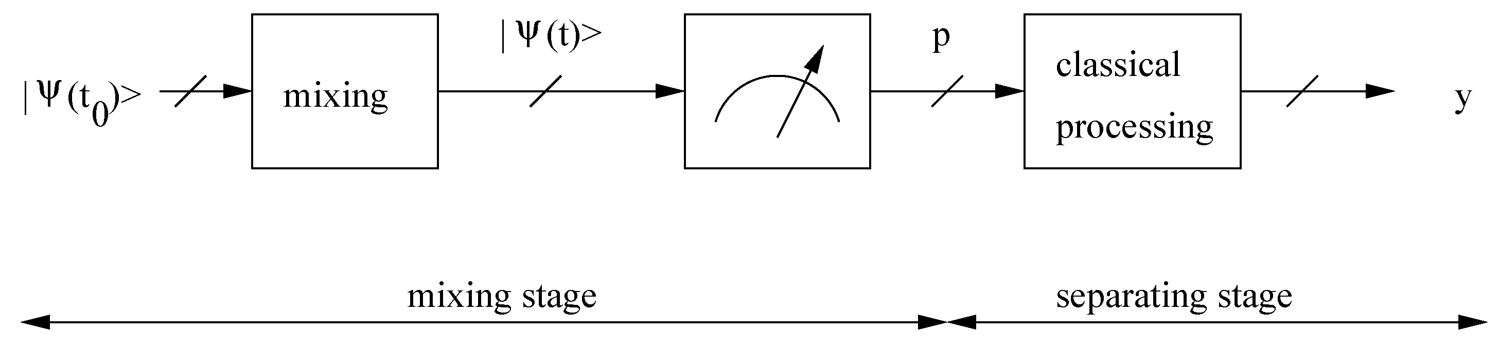In Section 4, we first make brief comments about the description of quantum states (including the existence of statistical mixtures as source states, in a more general context), about the act of measurement and about the physical realization of qubits with electron spins. We then discuss questions related to the probabilities of the possible results obtained in measurements of spin components, in the context of spins 1/2 as qubits. We first present their use when the Reader makes measurements at the Mixer output in order to restore the sources (cf. Figure 1). These measurements establish a link between the output of the Mixer and the classical world. It is stressed that while the macroscopic support of the results of measurements has a classical behaviour, the probabilities of these results obey quantum laws. We then establish an unentanglement criterion using probabilities, equivalent to the one established in Section 2 for the probability amplitudes $c_i$. It is shown that the $c_i$ coefficients can be expressed as functions of the probabilities of results in the measurements of well-chosen spin components. In Section 5, we derive the expression of the above unentanglement criterion for all possible source states, at the output of the so-called separating system, with respect to the parameters of both the cylindrical Heisenberg coupling, an abstract Mixer largely used in our previous papers, and that separating system.

In Part A.2 of the Appendix, the question of the applications of BQSS is addressed. Partly because the appearance of BQSS is recent, the subject of its applications is presently largely speculative. Two main subdomains should be distinguished. The first one is BQSS in a strict sense. It aims at recovering the source states and is the quantum counterpart of conventional BSS. The second subdomain focuses on an intermediate step possibly found in methods developed for BQSS and aiming at the knowledge of the mixer function or of its inverse. The corresponding classical problem is known as Blind Mixture Identification (BMI), a subfield of System Identification. The non-blind quantum version of System Identification is that already mentioned and well-established field of QIP called Quantum Process Tomography (as opposed to Quantum State Tomography). We recently introduced the quantum version of BMI, which we proposed to call Blind Quantum Process Tomography (BQPT).

2. An Unentanglement Criterion for a Qubit Pair

A superficial look may suggest that it is possible to restore the initial product state through State or Process Tomography (ST, PT). ST aims at determining a quantum state if a lot of copies of that state are available [20]. However, in BQSS, the Reader is unable to access the input of the Mixer, and ST is therefore obviously presently strictly useless. PT would presently consist of placing (preparing) successive well-defined and known quantum states at the input of the Mixer, thus operating in the non-blind mode (cf. [15], p. 202) and observing the corresponding signals at its output. However, in the BQSS problem, the Reader is strictly unable to operate that way, as he is unable to ask the Writer to prepare him the quite specific input states asked for by PT. Therefore, quantum tomography is unable to solve the BQSS problem, which needs dedicated methods (for more details, see [8]).

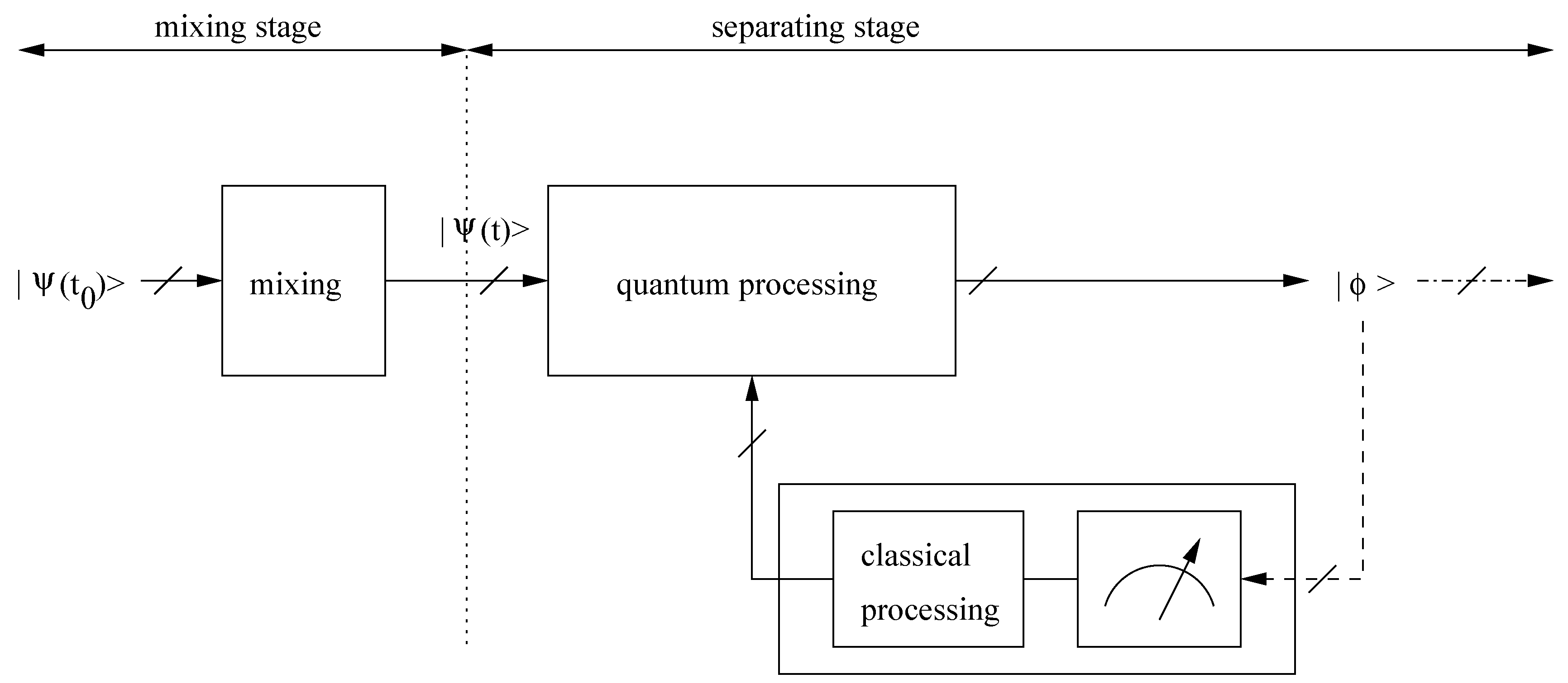
Up to now, in the BQSS problem, we developed two main approaches for both determination of the unknown parameter(s) of the mixing or separating system and source separation. In the first approach [7,8,11], the Reader measures observables, using the signals at the Mixer output (cf. Figure 1). The results, and properties associated with them, e.g., the probabilities of their occurrences, are kept upon a macroscopic device, e.g., the memory of a classical computer, and then used in a separating system. Since this macroscopic device and the separating system have a classical behaviour, we called this processing aimed at restoring the sources “classical-processing BQSS”. In the second, quite different, and more recently introduced approach [9,10,14], the quantum state at the Mixer output is sent to the input of a quantum-processing subsystem (cf. Figure 2), the inverting block of the separating system. This block is so designed that its output provides a quantum pure state equal to $\mid \mathsf{\Psi }\left(t_0\right)>$ (possibly up to some acceptable indeterminacies), after the adaptation phase.

From now on, the state spaces of two arbitrary qubits, called qubits 1 and 2, are denoted as ${\mathcal{E}}_1$ and ${\mathcal{E}}_2$, respectively. The possible (pure) states of the pair are the kets in ${\mathcal{E}}_1\otimes$ ${\mathcal{E}}_2.$ We assume that the qubits are physically realized with spins 1/2, which, e.g., allows us to speak of the spin component $s_{1z}$ or $s_{2z},$ but many results established hereafter keep true without this assumption. We introduce the orthonormal basis ${\mathcal{B}}_{+}$, {$\mid ++>,$ $\mid +->,$ $\mid -+>,\mid -->$}, where e.g., $\mid +->$ means $\mid 1+>\otimes \mid 2->$ and $\mid i,+>$, $\mid i,->$ are normed eigenkets of the $s_{iz}$ component of (reduced) spin $\overrightarrow{s_i}$ (with i = 1, 2), for the eigenvalues +1/2 and −1/2, respectively. Any pure pair state, entangled or not, may be expanded in ${\mathcal{B}}_{+}$ as

$$\mid \mathsf{\Psi }>=c_1\mid ++>+c_2\mid +->+c_3\mid -+>+c_4\mid -->,$$

(1)

where the complex coefficients $c_j$ (j = 1 to 4) respect ${\sum }_j$ $\mid c_j{\mid }^2$ $=1$. If a pure state or a statistical mixture of a bipartite system $S_{12}$ (parts $S_1$ and $S_2$) is described by a density operator $\rho$, the corresponding reduced traces ${\rho }_1=$ $T{r}_2\rho$ and ${\rho }_2$ $=T{r}_1\rho$ have all the mathematical properties of a density operator [2]. In addition, if $S_{12}$ is in a pure state, ${\rho }_1$ and ${\rho }_2$ have the same eigenvalues [21]. This pure state is unentangled if and only if its Schmidt number $N_S$ (the number of non-zero eigenvalues of ${\rho }_1$ and ${\rho }_2$) is equal to 1 [21]. We are particularly interested in the case when $\mid \mathsf{\Psi }>$ is the state found at the output of the inverting block. Then, any pure state may be expanded in the standard basis $\mathcal{B}+$ as in Equation (1), where the values of the $c_i$ coefficients are affected by both the coupling between the qubits and, during the adaptation phase, by the adaptation procedure. This adaptation phase typically consists of an iterative numerical algorithm, which aims at optimizing a continuous-valued function, traditionally called the “cost function”. For any given values of the adjustable parameters of the inverting block, the cost function measures a kind of “distance” between $\mid \mathsf{\Psi }>$ at the output of the inverting block and an unentangled pure state. The Schmidt unentanglement criterion cannot be used in our problem because the considered state remains (at least slightly) entangled throughout the adaptation procedure, and the Schmidt number thus remains higher than one. The Schmidt criterion provides a binary-valued unentanglement detector, with a Schmidt number equal to one or not and, if taking into account all possible integer values of $N_S$ beyond unentanglement detection, the Schmidt criterion provides a discrete-valued quantity. What we eventually need instead is a quantitative, continuous-valued, measure of that “distance” of the considered state with respect to unentanglement, in order to keep the adjustable parameter values of the inverting block, yielding the state which is the closest to unentanglement. Moreover, even if the Schmidt approach could be modified to this end, it would yield high computational complexity, as it would require one to diagonalize ${\rho }_1$ or ${\rho }_2$ for each of the quite numerous steps of the iterative adaptation algorithm. We avoid these issues as follows. Since the qubit pair is in a pure state, its partial traces ${\rho }_1$ and ${\rho }_2$ satisfy

$$\mathrm{Tr}{\rho }_1^2=\mathrm{Tr}{\rho }_2^2\le 1,$$

(2)

and the common value for $\mathrm{Tr}{\rho }_1^2$ and $\mathrm{Tr}{\rho }_2^2$ is 1 if and only if the pure state is unentangled (cf. [21]). One could think of using $\mathrm{Tr}{\rho }_1^2-1$ as a cost function. However, $\mathrm{Tr}{\rho }_1^2$ depends upon the $c_i$, which suggests one to try and establish an unentanglement criterion using the $c_i$ explicitly. To this end, we consider state $|\mathsf{\Psi }\rangle$ defined through Equation (1). When it is assumed that $|\mathsf{\Psi }\rangle$ is unentangled, i.e., that it can be written as

$$|\mathsf{\Psi }\rangle =(a|+\rangle +b|-\rangle )\otimes (c|+\rangle +d|-\rangle ),$$

(3)

then, in Equation (1), $c_1$ = $ac$, $c_2$ = $ad$, $c_3$ = $bc$, $c_4$ = $bd$, so $c_1{c}_4$ and $c_2{c}_3$ are both equal to $abcd$:

$$c_1{c}_4=c_2{c}_3.$$

(4)

Conversely, when it is assumed that Equation (4) is satisfied, if $c_1\ne 0$ then $|\mathsf{\Psi }\rangle$ may be written as

$$|\mathsf{\Psi }\rangle =c_1\left(\right|+\rangle +\frac{c_3}{c_1}|-\rangle )\otimes \left(\right|+\rangle +\frac{c_2}{c_1}|-\rangle ),$$

(5)

which means that $|\mathsf{\Psi }\rangle$ is then unentangled. If Equation (4) is satisfied and $c_1=0$, then $c_2=0$ and $c_3\ne 0$, or $c_3=0$ and $c_2\ne 0$, or $c_2$ = $c_3$ = 0, and in each case $|\mathsf{\Psi }\rangle$ is unentangled. Therefore, if the qubit pair is in a pure state $|\mathsf{\Psi }\rangle$ written as in Equation (1), then:

$$|\mathsf{\Psi }\rangle \mathrm{is}\mathrm{unentangled}⟺c_1{c}_4=c_2{c}_3.$$

(6)

This unentanglement criterion for a qubit pair pure state was used without justification in [9,10]. In Equation (1), $|\mathsf{\Psi }\rangle$ was expanded in the standard basis. It is possible instead to introduce e.g., the normed eigenvectors of $s_{1x}$ and $s_{2x},$ or more generally those of $s_{1u}$ and $s_{2v},$ the components of the spins along respective arbitrary directions $\overrightarrow{u}({\theta }_{1E},$ ${\phi }_{1E})$ and $\overrightarrow{v}({\theta }_{2E},$ ${\phi }_{2E})$, defined through their Euler angles. For each component, the possible results are again $\pm 1/2$. The possible results for the pair may be symbolically written as $(+u+v),$ $(+u-v),$ $(-u+v)$ and $(-u-v),$ and the corresponding probabilities as $P_{1uv},$ $P_{2uv},$ $P_{3uv},$ $P_{4uv.}$ Equation (1) is replaced by

$$|\mathsf{\Psi }\rangle =c_{1uv}|+u+v\rangle +c_{2uv}|+u-v\rangle +c_{3uv}|-u+v\rangle +c_{4uv}|-u-v\rangle .$$

(7)

With the same reasoning within the new basis, (6) is replaced by

$$|\mathsf{\Psi }\rangle \mathrm{is}\mathrm{unentangled}⟺c_{1uv}{c}_{4uv}=c_{2uv}{c}_{3uv}.$$

(8)

3. Random Quantum Sources and Their Independence

The qubits are again supposed to be physically realized with spins 1/2. Standard Electron Spin and Nuclear Magnetic Resonance (ESR, NMR) use a non-microscopic number of resonant spins, but methods have been proposed for more than twenty years in order to detect a single spin, particularly with Optically Detected Magnetic Resonance (ODMR [22,23]) or with Magnetic Resonance Force Microscopy (MRFM [24]), and more recently at low temperature (0.5 K) with Spin Excitation Spectroscopy [25], or even with ESR, in extreme conditions [26]. These approaches are still under development. Here, anticipating upon advances in spintronics, we rather consider a pair of spins, or even a single spin, submitted to a static magnetic field.

When speaking e.g., of a microwave source for satellite television, one speaks of the device emitting the microwave carrier. Similarly, the expression “laser source” generally refers to the device creating the coherent radiation. In conventional SS, “source” is an abbreviation for “source signal”. Furthermore, in Quantum SS with abstract qubits corresponding to physical spins 1/2, the word “source” does not refer to some atomic beam delivering atoms carrying an electron or nuclear magnetic moment, but still means “source signal”, then referring to some information from the quantum states of these qubits.

In conventional SS, an important concept is that of statistical independence of the sources, at the root of the frequent use of Independent Component Analysis (ICA) [27]. In [7,8,11], we postulated the existence of statistically independent quantum sources when using the classical-processing SS defined at the beginning of Section 2. Hereafter, we show that statistical independence may exist in that context. Quantum Mechanics (QM) does e.g., consider random operators, the matrix elements of which are random quantities (see the random lattice operators $F^{\left(q\right)}$ in the quantum description of the motions of nuclear moments in liquids, in the study of Spin-Lattice Relaxation (SLR), in [28]). As a simple model situation, a magnetic moment $\overrightarrow{\mu }$ associated with a single electron spin 1/2, with $\overrightarrow{\mu }$ $=-G$ $\overrightarrow{s}$ (isotropic $\overline{\overline{g}}$ tensor), placed in a Stern–Gerlach device, is now introduced. The static field is $\overrightarrow{B_0}$ = $B_0\overrightarrow{Z}$, with amplitude $B_0$. The system of interest consists of this spin and the magnet. Writing the Zeeman Hamiltonian as $h=-\overrightarrow{\mu }{\overrightarrow{B}}_0$ = $G{B}_0{s}_Z$ indicates that while the spin is a quantum object, the magnetic field is treated classically. The Writer first prepares the spin in the $|+Z\rangle$ eigenstate of $s_Z$ (eigenvalue $+1/2$). The moment is then received by the Reader, supposed to ignore the direction of $\overrightarrow{B_0}$, and who chooses some direction attached to the Laboratory as the quantization direction, called z (unit vector $\overrightarrow{u_z}$) and introduces a Laboratory-tied cartesian reference frame $xyz$, used to define ${\theta }_E$ and ${\phi }_E$, the Euler angles of $\overrightarrow{Z}$. Since the field is treated classically, ${\theta }_E$ and ${\phi }_E$ behave as classical variables, while $s_Z$ is an operator. The Reader measures $s_z$ $=\overrightarrow{s}\overrightarrow{u_z}$ (eigenstates: $|+\rangle$ and $|-\rangle$), and is interested in the probability $p_{+z}$ of getting $+1/2$. An elementary calculation indicates that

$$|+Z\rangle =r|+\rangle +\sqrt{1-r^2}{e}^{i\phi }|-\rangle ,$$

(9)

with

$$r=cos\frac{{\theta }_{2E}}{2},\phi ={\phi }_E,$$

(10)

and therefore $p_{+z}={cos}^2{\theta }_E/2.$ Once the direction of the magnetic field has been chosen, state $|+Z\rangle$ is then unambiguously defined. If this direction has a deterministic nature, r and $\phi$ are deterministic variables, and $|+Z\rangle$ may then be called a deterministic quantum state. If ${\theta }_E$ and ${\phi }_E$, defining the direction of $\overrightarrow{B_0}$ chosen by the Writer, obey probabilistic laws, one may consider that the quantum quantities r and $\phi$, which depend upon the classical Random Variables (RV) ${\theta }_E$ and ${\phi }_E$, do possess the properties of conventional, i.e., classical, RV. It may e.g., happen that they be uncorrelated, or even independent (which happens if ${\theta }_E$ and ${\phi }_E$ are independent). In addition, if ${\theta }_E$ and ${\phi }_E$ depend on time in a random way, r and $\phi$ are then random time functions. We are not strictly facing the quantum equivalent of a classical situation here. Rather, the stochastic character of the field direction, with classical nature, is reflected in the random behaviour of the quantum state expressed through Equation (9). Therefore, rather than a random operator, we meet here a random quantum state. The concept of a random state, if not the expression, was already used e.g., in the early and canonical books [29,30]. The probability $p_{+z}$, presently a function of the RV ${\theta }_E,$ is itself an RV. This results from both the randomness of the field direction and the standard probabilistic interpretation of QM. Probabilities of results of measurements for a qubit pair were treated as RV, without the present justification, in most of our previous papers, including [7,8,11].

If one measures the scalar observable O when the spin is in the state $|\mathsf{\Psi }\rangle =$ $\alpha |+\rangle +\beta |-\rangle$ = ${\Sigma }_k{f}_k|{\phi }_k\rangle$ (where k is associated with + and −), had the $f_k$ been deterministic the mean value would have been:

$$\langle \mathsf{\Psi }\left|O\right|\mathsf{\Psi }\rangle =\sum _{k,l}{f}_k^{*}{f}_l{O}_{kl},O_{kl}=\langle {\phi }_k\left|O\right|{\phi }_l\rangle .$$

(11)

Since the $f_k$ are random, one must moreover calculate the statistical mean, denoted as $\overline{\langle \mathsf{\Psi }\left|O\right|\mathsf{\Psi }\rangle }$:

$$\overline{\langle \mathsf{\Psi }\left|O\right|\mathsf{\Psi }\rangle }=\sum _{k,l}\overline{f_k^{*}{f}_l}{O}_{kl}=Tr\rho O,$$

(12)

where $\rho$ is the density operator, the matrix elements of which, in the $\left(\right|+\rangle$ , $|-\rangle )$ basis, are ${\rho }_{l,k}$ = $\overline{f_k^{*}{f}_l}$. Therefore, it is in principle possible to presently introduce a density operator, which is a non-random operator (its matrix elements are not random quantities, but statistical averages). However, this does not present any interest, since in the BQSS problem examined up to now, the Reader knows that e.g., qubit 1 has been prepared in a pure state, but does not know the values of the ${\rho }_{ij}$ coefficients in any basis, and is consequently unable to choose a basis in which $\rho$ would be diagonal. It is simpler to keep speaking of a random pure state.

As a model situation, we now consider two spins 1/2 numbered 1 and 2, each with conditions similar to the previous ones, with fields along directions with respective unit vectors $\overrightarrow{Z_1}({\theta }_{1E},{\phi }_{1E})$ and $\overrightarrow{Z_2}({\theta }_{2E},{\phi }_{2E})$, and each spin initially prepared in the state

$$|{\psi }_i\left(t_0\right)\rangle =r_i|i+\rangle +\sqrt{1-r_i^2}{e}^{i{\phi }_i}|i-\rangle ,i=1,2,$$

(13)

where $|i+\rangle$ and $|i-\rangle$ are the eigenkets of $s_{iz}$, the component of $\overrightarrow{s_i}$ along the quantization direction, for the eigenvalues 1/2 and −1/2, respectively. For the same reason, if the field directions are random, $r_1,$ ${\phi }_1,$ $r_2$ and ${\phi }_2$ have the properties of conventional RV. If (${\theta }_{1E},{\phi }_{1E}$) and (${\theta }_{2E},{\phi }_{2E}$) are mutually statistically independent, the same is then true for the couples of RV ($r_1,$ ${\phi }_1$) and ($r_2,$ ${\phi }_2$). In addition, if e.g., ${\theta }_{1E}$ and ${\phi }_{1E}$ are independent, the same is true for $r_1$ and ${\phi }_1$ (cf. Equation (10)). These properties are of major importance for our quantum-source independent component analysis (QSICA) methods described in [11]. We may then say that the initial state of each qubit is random, i.e., that in Equation (13) $r_i$ and ${\phi }_i$ are RV. When considering the preparation of a pair of qubits each in a pure state, one may assume either a deterministic or a random direction for each magnetic field. This discussion shows that the relevant concept, in the latter case, is that of random quantum states, rather than that of random quantum operators mentioned earlier in this section.

Keeping our assumption of a pair of qubits each prepared in a pure state, we now consider the second approach for the adaptation and inversion phases (cf. the beginning of Section 2 and Figure 2), with a quantum state $|\mathsf{\Phi }\rangle$ present at the output of the inverting block. The presence of $|\mathsf{\Phi }\rangle$ and the Reader’s final aim, the recovery of the initial pure state, prompts the Reader: (1) to speak of a deterministic or random pure state, rather than to use a density operator; (2) to consider that the first constraint to be respected in BQSS is then the very existence of an unentangled state at the output of this inverting block. If unentanglement has first been achieved, then and only then is it possible to speak of a deterministic or random state for each part of that product state. While entanglement has no classical counterpart, the following point may be noted here: if a bipartite system is in a pure (deterministic) state $|\mathsf{\Phi }\rangle ,$ to which a density operator $\rho$ $=|\mathsf{\Phi }\rangle \langle \mathsf{\Phi }|$ corresponds, $|\mathsf{\Phi }\rangle$ is unentangled if and only if the partial traces ${\rho }_1$ and ${\rho }_2$ satisfy the equality $\rho ={\rho }_1\otimes {\rho }_2$ [31]. This unentanglement condition is reminiscent of the relation $\rho =$ ${\rho }_1$·${\rho }_2$ between $\rho$, the joint probability density function of independent classical RV $X_1$ and $X_2,$ and ${\rho }_1$ and ${\rho }_2,$ the respective marginal probability density functions. Presently, operators replace functions, a tensor product replaces the ordinary product, and this reminiscence reflects the existence of a classical analogue to unentangled states. Condition (4) for unentanglement was established using spins 1/2, but is valid for any pair of two-level systems. This discussion suggests that, in the BQSS problem, when considering a pair of qubits prepared in a pure state, and moreover using the second approach of Section 2 for adaptation and inversion, instead of trying to directly import ICA methods into the BQSS context, one should focus on disentanglement at the output of the inverting block, which recently led us to introduce a disentanglement-based separation principle [9,10].

In the next section, use will be made of the number of real independent parameters necessary to define an arbitrary normed ket $|\mathsf{\Psi }\rangle$ in ${\mathcal{E}}_1\otimes {\mathcal{E}}_2,$ written as in Equation (1), and a ket in ${\mathcal{E}}_1\otimes {\mathcal{E}}_2$ forced to be unentangled. These numbers are specified hereafter. An arbitrary normed ket $|\mathsf{\Psi }\rangle$ in ${\mathcal{E}}_1\otimes {\mathcal{E}}_2$ depends upon the four complex quantities $c_1$ to $c_4$ linked through two relations between real numbers (${\sum }_i\mid c_i{\mid }^2$ is equal to $1,$ and $|\mathsf{\Psi }\rangle$ and $e^{i\phi }|\mathsf{\Psi }\rangle ,$ with $\phi$ an arbitrary real quantity, should be considered identical). An arbitrary normedket $|\mathsf{\Psi }\rangle$ in ${\mathcal{E}}_1\otimes {\mathcal{E}}_2$ therefore depends upon six real independent parameters. If it is forced to be unentangled, it has to satisfy the equality $c_1{c}_4=c_2{c}_3$ between complex quantities. An unentangled normed ket $|\mathsf{\Psi }\rangle$ therefore depends upon fourreal parameters. This corresponds to the fact that $|\mathsf{\Psi }\rangle$ is then restricted to the form $|\mathsf{\Psi }\rangle =$ $|{\psi }_1\rangle \otimes |{\psi }_2\rangle ,$ where the normed kets $|{\psi }_1\rangle$ and $|{\psi }_2\rangle ,$ describing the state of qubits 1 and 2, respectively, each depend upon two real parameters $(r_1,{\phi }_1),$ $(r_2,{\phi }_2)$ (cf. Equation (13)).

4. BQSS and Probabilities in Spin Component Measurements

4.1. Some General Considerations

Faced with the variety of existing interpretations of QM, Fuchs and Peres have argued that “quantum theory needs no interpretation” [32]. Concerning the question of interpreting QM, one may distinguish between claims that can be experimentally tested (i.e., confirmed or refuted) through experience, and those which cannot. This may be illustrated by an instance from the early days of QM, related to the measurement act. At first, Bohr apparently introduced some dichotomy between the quantum system of interest and the classical behaviour of the apparatus. Chapter VI of Von Neumann’s 1932 book [30] was perhaps the first attempt to treat the system of interest and the apparatus (with a so-called pointer) as a single system obeying the laws of QM. However, in his book, Von Neumann also introduced a postulate (wave-function reduction) specifiying the state of the system of interest at the end of the measurement. Since then, this postulate has been criticized, first by Margenau, who introduced the concept of preparation, to be distinguished from the one of measurement, and who insisted that e.g., when a photon is absorbed, the measurement act does not bring the photon into a new state, but destroys it [33,34]. The measurement act has been largely debated, including recent discussions through the concept of decoherence (see e.g., [1,21]). When trying to develop the domain of BQSS, we got some control of the proposed separation methods, through simulations, but we moreover tried to avoid using ideas linked with some specific “interpretation” of QM. In [8], we did mention Von Neumann’s book and the irreversible behaviour of the system during measurements, but, after getting a result through some measurement upon a qubit pair, we never used the state of that qubit pair at the end of that measurement. On the contrary, after such a measurement, the qubit pair was often (in an abstract process) submitted to a new preparation, which is not linked to any specific interpretation of QM.

In the previous sections, the concepts of a pure state and a statistical mixture were both used. The concept of a statistical mixture may be introduced through a different and more general situation [35] than the one used in Section 3. The system of interest S and its environment E are viewed as a global quantum system $\mathsf{\Sigma }$. If S and E are uncoupled, and isolated from the rest of the world, and have been separately prepared in a pure state at time $t_a$, then they evolve separetely, each in a (time-dependent) pure state. If, after $t_a$, a coupling between S and E exists between some times $t_b$ and $t_c,$ then from $t_b$ on their state generally becomes entangled. In addition, if, starting from $t_c$, one focuses upon the behaviour of S, use of the partial trace tool shows that everything then occurs as if S were in a state of statistical mixture described by a well-chosen density operator, obeying the Von Neumann equation. If one takes the qubit pair as S, up to now we did not discuss the BQSS problem found when the Writer proposes the qubit pair in a state described by a statistical mixture resulting from some past interaction with its environment.

In recent discussions about the measurement problem, the concept of decoherence [21] was used for discussing the effect of a transfer of energy from the system to its environment, an irreversible phenomenon corresponding to SLR in the ESR/NMR context (with, in the simplest situations, a characteristic time called $T_1$) [28,36]. In our previous papers and in the present one, starting from time $t_0$ when the Writer operates, then, at the chosen time scale, the qubit pair is assumed to be isolated from its environment.

In the ESR/NMR domain, a well-known situation exists when a collection of identical (nuclear or electron) spins placed in a fixed resonant magnetic field are transiently submitted to an intense, oscillating magnetic field with a frequency equal to (or near) its resonant value, and with well-chosen polarization. If each spin is coupled to the magnetic fields only, at the end of the pulse the density matrix (written in the basis in which the static Zeeman Hamiltonian is diagonal) describing the state of these spins possesses non-diagonal elements, called coherences. If a weak internal coupling (spin-spin coupling) such as the dipolar magnetic coupling exists between the spins, and if it is able to manifest itself at a time scale allowing one to neglect SLR, it progressively induces a decrease of the coherences, a reversible phenomenon allowing spin echo techniques.

There is presently a second reason for referring to these behaviours in the MR domain, namely the fact that DiVincenzo suggested the use of electron spins for the physical realization of qubits more than twenty years ago [37]. Between two neighbouring electron spins, there may exist a strong exchange interaction, a strictly quantum phenomenon historically first identified by Heisenberg in magnetically ordered materials. This is the first reason for our choice of a Heisenberg coupling in the BQSS problem. The second one is that, on the formal side, the version of the Heisenberg Hamiltonian with spherical or cylindrical symmetry, simple enough to be used in theoretical works, may serve as a benchmark in that BQSS problem. It should be recalled that an Ising coupling, simpler to manipulate theoretically than the Heisenberg one, was present in the DiVincenzo 1995 paper, where it helped in the operating process, while the presence of the Heisenberg coupling is undesired and should be compensated for in the BQSS context.

It is well-known that the ESR lines of transition ions in insulators at moderate concentrations are broadened by the dipolar magnetic coupling between the electron spins, the exchange interaction being negligible then. In concentrated samples, exchange is stronger than dipolar coupling and produces a narrowing of the lines [36]. Dipolar coupling is long ranged and anisotropic, which should lead to heavy theoretical treatments if considering a three-dimensional configuration in the BQSS context. Future technological developments could possibly make e.g., the consideration of a planar square lattice of dipolar coupled spins meaningful in that context.

4.2. Probabilities in Measurements, Classical versus Quantum World

In this subsection, we are interested in our first approach as defined in Section 2, with measurements at the Mixer output (cf. Figure 1). We specifically consider the solutions to BQSS discussed in [7,8,11], with two spins 1/2, each prepared in a pure state at $t_0$, then submitted to an undesired Heisenberg cylindrical coupling [28,38] (axial component: $J_z$, normal component: $J_{xy}$, cf. Equation (4) and Appendix E of [8], and [36]), and measurements of $s_{1z}$ and $s_{2z}$ at the output of the formal Mixer at $t_1$. The probabilities of obtaining $(+1/2,+1/2)$, $(+1/2,-1/2)$, $(-1/2,+1/2)$ and $(-1/2,-1/2)$ are denoted, respectively, as $p_1,$ $p_2,$ $p_3$ and $p_4$ (as in [8], while in [7] e.g., our present $p_4$ was denoted as $p_2$). We keep Equation (13) for both qubits, with the choice ${\phi }_1=0$. One then gets [8]:

$$p_1=r_1^2{r}_2^2,p_4=(1-r_1^2)(1-r_2^2).$$

(14)

$p_2$ depends upon a mixing parameter $v=$ sgn$(cos{\mathrm{\Delta }}_E)sin{\mathrm{\Delta }}_E$, with [8] ${\mathrm{\Delta }}_E=-J_{xy}(t_1-t_0)/\hslash$. This expression for ${\mathrm{\Delta }}_E$ may be vizualized as the opposite of the phase rotation $\mathrm{\Delta }\varphi$ = $\omega (t_1-t_0)$ between states coupled by a Hamiltonian term with energy $J_{xy}$, during the time interval $(t_1-t_0)$, with $\omega$ given by the Planck–Einstein relation $\omega =J_{xy}/\hslash$. Probability $p_2$ satisfies

$$p_2=r_1^2(1-r_2^2)(1-v^2)+(1-r_1^2)r_2^2{v}^2-2r_1{r}_2\sqrt{1-r_1^2}\sqrt{1-r_2^2}\sqrt{1-v^2}vsin{\mathrm{\Delta }}_I$$

(15)

and, with our choice for ${\phi }_1,$ ${\mathrm{\Delta }}_I=$ ${\phi }_2.$

In Equation (13), which describes the initial state of the qubit pair, $r_1,$ $r_2,$ ${\phi }_1$ and ${\phi }_2$, are used to define probability amplitudes, i.e., quantum quantities. Expressions (14) and (15) show that $p_1,$ $p_4$ and $p_2$ depend upon both $r_1$ and $r_2,$ and that $p_2$ moreover depends upon ${\mathrm{\Delta }}_I$ and therefore the probabilities clearly follow quantum laws. This instance illustrates the distinction to be made between the quantum status of these probabilities and the validity of the classical approximation for the physical supports that store them. In [7,8,11], once $r_1,$ $r_2$ and ${\mathrm{\Delta }}_I$ were known, the initially prepared qubit states were completely known, and in the context of classical-processing BQSS, we called $r_1,$ $r_2$ and ${\mathrm{\Delta }}_I$ the sources (cf. Section 3) in order to focus on the quantities used in the SS process.

The concept of RV is often used in a classical context. Since on the contrary probabilities $p_1$, $p_4$ and $p_2$ follow quantum laws, treating them as RV does not go without saying. However, Equations (14) and (15) establish that when $r_1,$ $r_2$, ${\phi }_2$ are RV (cf. Section 3) the same is true for $p_1,$ $p_4$ and $p_2$. They also indicate that $p_1$, $p_4$ and $p_2$ depend upon both $r_1$ and $r_2,$ and that $p_2$ also depends upon ${\mathrm{\Delta }}_I.$ When $J_{xy}=0$ (Ising Hamiltonian $-2J{s}_{1z}{s}_{2z}$), then $v=0$ and, for the state at the Mixer output, $p_1{p}_4=p_2{p}_3,$ which can be interpreted as follows. The four states defining the ${\mathcal{B}}_{+}$ basis are then eigenstates of the Hamiltonian, but time evolution introduces phase differences, and it can be verified that the state at the Mixer output is entangled (except if, accidentally, $J(t_1-t_0)/\hslash =k\pi ,$k being an integer). However, when measuring $s_{1z}$ and $s_{2z}$, the probability of getting $(1/2,1/2)$ is then time-independent, which is also true for the probabilities of getting $(1/2,-1/2),$ $(-1/2,1/2)$ or $(-1/2,-1/2).$ Therefore, both products $p_1{p}_4$ and $p_2{p}_3$ are time-independent, and since $p_1{p}_4$= $p_2{p}_3$ at $t_0,$ because the qubit pair is then in a product state, this equality is preserved as time goes on, although the state has become entangled.

In the end, these measurements made at the output of the Mixer establish a bridge between the classical and the quantum worlds, the results being kept on macroscopic devices for which the classical approximation is valid, while the probabilities of their occurrences follow quantum laws.

4.3. An Unentanglement Criterion Using Probabilities

The unentanglement criterion expressed through Equation (4) uses the $c_i$ coefficients, i.e., probability amplitudes. However, measurements give access to probabilities, not to probability amplitudes, and the question of establishing whether this unentanglement criterion could be formulated with probabilities (of the results from spin component measurements) therefore seems relevant. State $|\mathsf{\Phi }\rangle$ being present at the ouput of the inverting block, and the components $s_{1u}$ and $s_{2u}$ being then measured, we denote the probabilities of obtaining $(1/2,1/2)$, $(1/2,-1/2$), $(-1/2,1/2)$ and $(-1/2,-1/2)$ as $P_{1u},$ $P_{2u},$ $P_{3u},$ $P_{4u}$, respectively, and the corresponding eigenstates of $s_{1u}$.$s_{2u}$ as $|+u,+u\rangle ,$ $|+u,-u\rangle ,$ $|-u,+u\rangle$ and $|-u,-u\rangle$. If e.g., $s_{1x}$ and $s_{2x}$ are measured, the probabilities are denoted as $P_{ix}$, with $i=1$ to $4.$ In Section 3, it was said that an unentangled normed ket $|\mathsf{\Psi }\rangle$ in ${\mathcal{E}}_1\otimes {\mathcal{E}}_2$ possesses four degrees of freedom. Taking the squared modulus of each member of the equality $c_1{c}_4=c_2{c}_3$ leads to

$$P_{1z}{P}_{4z}=P_{2z}{P}_{3z}.$$

(16)

Then, taking $\overrightarrow{u}$ and $\overrightarrow{v}$ of Section 2 both along direction $x,$ we know that $c_{1x}{c}_{4x}=c_{2x}{c}_{3x}$ for an unentangled state (cf. Equation (8)), and therefore that

$$P_{1x}{P}_{4x}=P_{2x}{P}_{3x}.$$

(17)

Equation (16) together with (17) is however weaker than condition $c_1{c}_4=c_2{c}_3,$ as can be tested by considering the following state:

$$|{\mathsf{\Psi }}_{i-i11}\rangle =\frac{1}{2}\left(i\right|++\rangle -i|+-\rangle +|-+\rangle +|--\rangle ).$$

(18)

$|{\mathsf{\Psi }}_{i-i11}\rangle$ is entangled since $c_1{c}_4=-$$c_2{c}_3.$ It can be written

$$|{\mathsf{\Psi }}_{{}_{i-i11}}\rangle =\frac{1}{2}\left(\right|+x,+x\rangle +i|+x,-x\rangle -|-x,+x\rangle +i|-x,-x\rangle ).$$

(19)

Equation (19) shows that the four probabilities $P_{ix}$ attached to $|{\mathsf{\Psi }}_{i-i11}\rangle$ are all equal to $1/4.$ Therefore, $|{\mathsf{\Psi }}_{i-i11}\rangle$ satisfies (16) and (17), while being entangled.

The two qubits being in the state $|\mathsf{\Psi }\rangle$ expressed through (1), one may decide to treat the three orthogonal directions on the same footing, measuring successively $s_x$ for both spins, then, in a new set of preparations/measurements, $s_y$ for both spins, and finally $s_z$ for both spins. The probabilities of obtaining ($1/2,1/2)$), ($1/2,-1/2$), ($-1/2,1/2$), ($-1/2,-1/2$), respectively, when measuring $s_{1k}$ and $s_{2k}$ (with k successively equal to $x,$ $y,$ and z), will be denoted as $P_{1k},$ $P_{2k},$ $P_{3k}$ and $P_{4k}.$ For e.g., the entangled state $|{\mathsf{\Psi }}_{i-i11}\rangle$ , as $P_{1z}{P}_{4z}=P_{2z}{P}_{3z}$ and $P_{1x}{P}_{4x}=P_{2x}{P}_{3x},$ the hope is that entanglement can be detected thanks to $P_{1y}{P}_{4y}$ ≠ $P_{2y}{P}_{3y},$ but, in fact, the four $P_{iy}$ are equal to $1/4$. Therefore, measuring the same spin component for both qubits, successively for $x,$ y and z, fails to allow us to build up an unentanglement criterion.

However, since two spins are present, there is still the possibility of not systematically measuring the same spin component for both spins. One chooses to measure successively $s_z$ for both spins, then $s_{1z}$ and $s_{2x}$ in a new set of preparations/measurements, and finally $s_{1z}$ and $s_{2y}.$ The presence of the $s_{1z}$ measurement in each of these sets corresponds to recognizing that (1) uses the standard basis. The probabilities of obtaining (1/2, 1/2), (1/2, −1/2), (−1/2, 1/2), (−1/2, −1/2), respectively, when measuring $s_{1i}$ and $s_{2j}$ (with $i=z,$ $x,$ or $y,$ and $j=z,$ $x,$ or $y)$ will be denoted as $P_{1ij},$ $P_{2ij},$ $P_{3ij}$ and $P_{4ij}.$ Denoting the $c_i$ introduced in Equation (1) as $c_i={\rho }_i{e}^{i{\psi }_i},$ then from Equation (4) it is known that $|\mathsf{\Psi }\rangle$ is unentangled if and only if

$$\{{\rho }_1{\rho }_4={\rho }_2{\rho }_3\mathrm{and}{\psi }_1+{\psi }_4={\psi }_2+{\psi }_3\mathrm{mod}2\pi \}.$$

(20)

Measuring {$s_{1z},$ $s_{2z}$} allows us to know the moduli $\mid c_i{\mid }^2={\rho }_i^2$ in (1), and to express the first equality in Equation (20) as

$$P_{1zz}{P}_{4zz}=P_{2zz}{P}_{3zz}.$$

(21)

The $P_{kzx}$ and $P_{kzy}$ (with $k=1$ to 4), when expressed as functions of the moduli ${\rho }_l$ and angles ${\psi }_m,$ depend upon trigonometric functions of the ${\psi }_m$ angles. For instance, for any state $|\mathsf{\Psi }\rangle$ entangled or not

$$2P_{1zx}=({\rho }_1^2+{\rho }_2^2)+2{\rho }_1{\rho }_{2}cos({\psi }_1-{\psi }_2).$$

(22)

When expressing unentanglement through probabilities, one then has to try and respect both $cos\alpha$ = $cos\beta$ and $sin\alpha$ = $sin\beta$ with $\alpha$ and $\beta$ values compatible with the equality ${\psi }_1+{\psi }_4={\psi }_2+{\psi }_3$, rather than to respect the equality ${\psi }_1+{\psi }_4={\psi }_2+{\psi }_3$ (mod $2\pi$) itself. If it is first known that simultaneously $P_{1zz}{P}_{4zz}=P_{2zz}{P}_{3zz}$ and $P_{1zx}{P}_{4zx}=P_{2zx}{P}_{3zx}$ are true, then one immediately deduces that $cos({\psi }_1-{\psi }_2)=cos({\psi }_3-{\psi }_4)$. In addition, if $P_{1zy}{P}_{4zy}=P_{2zy}{P}_{3zy}$ replaces the second equality, one deduces that $sin({\psi }_1-{\psi }_2)=sin({\psi }_3-{\psi }_4)$. Therefore, when the three equalities between probability products are satisfied, then ${\rho }_1{\rho }_4={\rho }_2{\rho }_3$ and ${\psi }_1+{\psi }_4={\psi }_2+{\psi }_3$ (mod $2\pi$). Conversely, if $|\psi \rangle$ is unentangled, then Equation (8) implies that $P_{1zj}{P}_{4zj}=P_{2zj}{P}_{3zj}$, with $j=z,x,y$ respectively. Finally,

$$c_1{c}_4=c_2{c}_3⟺\{P_{1zj}{P}_{4zj}=P_{2zj}{P}_{3zj},\mathrm{with}j=x,y,z\}.$$

(23)

The equivalence therefore is between a single relation between probability amplitudes and a triplet of relations between probabilities. This criterion, although established in the context of BQSS, has the same general validity as Equation (4).

Use of criterion (23) necessitates successive measurements first of $s_{1z}$ and $s_{2z}$, then (after new preparations) of $s_{1z}$ and $s_{2x},$ and finally (again after new preparations) of $s_{1z}$ and $s_{2y}$, in order to successively estimate first the $P_{izz}$ probabilities, then the $P_{izx}$ and finally the $P_{izy}$. One must measure $s_{1z}$ each time, because (1) getting e.g., ($+1/2$, $-1/2$) when measuring $s_{1z}$ and $s_{2z}$ is an event to be distinguished from the one realized when measuring $s_{1z}$ and $s_{2x}$ and getting ($+1/2$, $-1/2$), (2) results of measurements of $s_{1z}$ and $s_{2x}$ are independent only if $|\mathsf{\Psi }\rangle$ is unentangled, which precisely can’t be assumed when Equation (23) is to be used.

The two distinguishable spins were made to play different roles in the process, which led to Equation (23) (systematic measurement of $s_{1z}$). This dissymmetry is only partial, as Equation (23) can be replaced by a version obtained by exchanging the spin numbers. The next subsection makes a symmetrical use of measurements of spin components, allowing one to get the values of both the ${\rho }_i$ moduli and the ${\psi }_i$ angles for the $c_i$ coefficients in Equation (1).

4.4. Knowing 2-Qubit Pure States from $s_{ij}$ Measurements

If a qubit pair physically realized with spins 1/2 is known to be in an arbitrary pure state described by $|\mathsf{\Psi }\rangle$ written as in Equation (1), with $c_i={\rho }_i{e}^{i{\psi }_i}$ and $i=1$ to $4,$ then in order to know $|\mathsf{\Psi }\rangle$, one should know three moduli ${\rho }_i$ and three angles ${\psi }_i$. Accessing these six real quantities is more demanding than testing $|\mathsf{\Psi }\rangle$ unentanglement, since once these quantities are known, it is always possible to know whether $|\mathsf{\Psi }\rangle$ is unentangled, by testing whether both equalities ${\rho }_1{\rho }_4={\rho }_2{\rho }_3$ and ${\psi }_1+{\psi }_4$ $={\psi }_2+{\psi }_3$ are satisfied. On the contrary, when one focuses upon entanglement, these two equalities may be found to be satisfied, while the values of the ${\rho }_i$ and ${\psi }_i$ are unknown. In the previous subsection, an unentanglement criterion using only probabilities in the measurements of the $s_{ij}$ components, equivalent to the $c_1{c}_4=c_2{c}_3$ criterion, was given. Its existence suggests the following question: is it possible to access these six real quantities using only probabilities of results in the measurements of the spin components? We are going to show that the answer is yes. It is already known that measurements of both $s_{1z}$ and $s_{2z}$ give access to the moduli ${\rho }_i,$ through the probabilities $P_{izz}$ introduced in Section 4.3. One is left with e.g., determining the three angle differences (${\psi }_1-{\psi }_3)$, (${\psi }_2-{\psi }_3)$ and (${\psi }_4-{\psi }_3)$ from well-chosen probabilities. We first consider measurements of $s_{1z}$ and $s_{2i},$ with $i=x$ or $y,$ as in Section 4.3. When measuring $s_{1z}$ and $s_{2x},$ the probabilities of getting $(1/2,$ $1/2$) and $(-1/2,$ $1/2$) are, respectively,

$$P_{1zx}=\frac{1}{2}\mid c_1+c_2{\mid }^2,P_{3zx}=\frac{1}{2}\mid c_3+c_4{\mid }^2,$$

(24)

which leads to

$$cos({\psi }_1-{\psi }_2)=\frac{2P_{1zx}-P_{1zz}-P_{2zz}}{2\sqrt{P_{1zz}{P}_{2zz}}},cos({\psi }_3-{\psi }_4)=\frac{2P_{3zx}-P_{3zz}-P_{4zz}}{2\sqrt{P_{3zz}{P}_{4zz}}}.$$

(25)

Similarly, when measuring $s_{1z}$ and $s_{2y},$ the probabilities of getting $(1/2,$ $1/2$) and $(-1/2,$ $1/2$) are, respectively,

$$P_{1zy}=\frac{1}{2}\mid c_1-i{c}_2{\mid }^2,P_{3zy}=\frac{1}{2}\mid c_3-i{c}_4{\mid }^2,$$

(26)

which leads to

$$sin({\psi }_1-{\psi }_2)=-\frac{2P_{1zy}-P_{1zz}-P_{2zz}}{2\sqrt{P_{1zz}{P}_{2zz}}},sin({\psi }_3-{\psi }_4)=-\frac{2P_{3zy}-P_{3zz}-P_{4zz}}{2\sqrt{P_{3zz}{P}_{4zz}}}.$$

(27)

Expressions (25) and (27) allow us to know both $({\psi }_1-{\psi }_2)$ and $({\psi }_3-{\psi }_4)$ (mod $2\pi$).

Now, exchanging the roles of spins 1 and 2, we successively measure {$s_{1x},$ $s_{2z}\}$ and (after new preparations) {$s_{1y},s_{2z}\}.$ The probabilities of getting $(1/2,$ $1/2$) in these measurements are, respectively,

$$P_{1xz}=\frac{1}{2}\mid c_1+c_3{\mid }^2,P_{1yz}=\frac{1}{2}\mid c_1-i{c}_3{\mid }^2,$$

(28)

which leads to

$$cos({\psi }_1-{\psi }_3)=\frac{2P_{1xz}-P_{1zz}-P_{3zz}}{2\sqrt{P_{1zz}{P}_{3zz}}},sin({\psi }_1-{\psi }_3)=-\frac{2P_{1yz}-P_{1zz}-P_{3zz}}{2\sqrt{P_{1zz}{P}_{3zz}}}.$$

(29)

$({\psi }_1-{\psi }_3)$ is therefore known (mod 2$\pi )$.

If one wants to identify not the state at the Mixer input but a pure state at the Inverter output, State Tomography (ST) may in principle be used. However, it is far simpler to make measurements for the five {$s_{1i}$, $s_{2j}$} pairs just considered and to access the corresponding probabilities, than to use ST. The reason is that ST claims to be valid for any quantum state, and therefore does not take advantage of the fact that the qubit pair is presently known to be in a pure state. The dimension of the state space of the qubit pair being four, then, for ST, one has to introduce sixteen operators, namely the Identity, the six operators $s_{1i}$ and $s_{2j}$ (with $i=x,$ $y,$ z, and $j=x,$ $y,$ z), and the nine products $s_{1i}{s}_{2j}$ [20]. One should determine experimentally fifteen mean values, giving access to fifteen independent real values together defining the density operator describing the qubit pair state (three diagonal real elements, and six non-diagonal complex elements).

The simpler state estimation procedure proposed in this section therefore opens the way to new classes of BQSS methods, that we just started to explore in [12,13], and then applying this procedure to the Mixer output.

5. Disentanglement and Cylindrical-Symmetry Heisenberg Coupling

In Section 4.2, we considered measurements made at the Mixer output. We now come to the method for BQSS used, e.g., in [9], with classical processing in the adapting block of the separating system, using the notations of [9]. $\left|\mathsf{\Psi }\right(t_0)\rangle$, the initial product state of the qubit pair, is given by Equation (1), with the values of the coefficients $c_i$ (in the ${\mathcal{B}}_{+}$ basis) taken at $t_0$ and denoted as $c_i\left(t_0\right)$. These components form the source vector

$$C_{+}\left(t_0\right)={[c_1\left(t_0\right),c_2\left(t_0\right),c_3\left(t_0\right),c_4\left(t_0\right)]}^T,T:\mathrm{transpose}.$$

(30)

Similarly, the state at the Mixer output at time t, here denoted as $\left|\mathsf{\Psi }\right(t)>$, is given by Equation (1), with the values of the coefficients $c_i$ (in the ${\mathcal{B}}_{+}$ basis) taken at t and denoted as $c_i\left(t\right)$. The coupling-induced transition from state $\left|\mathsf{\Psi }\right(t_0)\rangle$ to $\left|\mathsf{\Psi }\right(t)\rangle$ is interpreted as the transformation induced by the Mixer, leading to the appearance of $\left|\mathsf{\Psi }\right(t)\rangle$ at its output. In the same basis, $\left|\mathsf{\Psi }\right(t)\rangle$ is described by the column vector $C_{+}\left(t\right)$ given by (30), with t replacing $t_0.$ In the matrix formalism, the relation between $C_{+}\left(t_0\right)$ and $C_{+}\left(t\right)$ is written as

$$C_{+}\left(t\right)=M{C}_{+}\left(t_0\right),$$

(31)

where the square fourth-order matrix M describes the effect of the coupling. In [8], it was shown that when the coupling may be described by a Heisenberg cylindrical Hamiltonian, then $M=QD{Q}^{-1},$ where $Q=Q^{-1}$ is a square matrix with the following non-zero matrix elements:

$$Q_{11}=Q_{44}=1,Q_{22}=-Q_{33}=Q_{23}=Q_{32}=\frac{1}{\sqrt{2}},$$

(32)

and D is a Diagonal square matrix with its diagonal elements equal to $D_{ii}=e^{-i{\omega }_i(t-t_0)}$ ($i=1$...4), the ${\omega }_i$ being real quantities depending upon $J_z$ and $J_{xy}$, with generally unknown numerical values. The input of the inverting block then receives this state $\left|\mathsf{\Psi }\right(t)\rangle .$ Its output provides a state $|\mathsf{\Phi }\rangle$ described in the ${\mathcal{B}}_{+}$ basis by a column vector $C,$ with

$$C=U{C}_{+}\left(t\right)=UM{C}_{+}\left(t_0\right),$$

(33)

where the square matrix $U$ (Unmixing matrix) describes the effect of the inverting block of the separating system. If it is possible to choose U in the form $U=M^{-1}$, then $|\mathsf{\Phi }\rangle$ will be equal to $\left|\mathsf{\Psi }\right(t_0)\rangle .$ However, strictly speaking, operating this way is impossible because $M=QDQ,$ and D is unknown. In [9], the inverting block was formally built using a chain of quantum gates globally realizing matrix U in the form $U=Q\tilde{D}Q,$ where $\tilde{D}$ is a diagonal matrix with its four diagonal elements ${\tilde{D}}_{ii}$ ($i=1...4$) equal to

$${\tilde{D}}_{ii}=e^{i{\gamma }_i},{\gamma }_i:\mathrm{free}\mathrm{real}\mathrm{parameters}.$$

(34)

$\tilde{D}D=\mathrm{\Delta }$ is therefore a diagonal matrix with diagonal elements ${\mathrm{\Delta }}_{ii}=e^{i{\delta }_i},$ where

$${\delta }_i={\gamma }_i-{\omega }_i(t-t_0).$$

(35)

The $\tilde{D}$ matrix and the adaptation phase were introduced because it is not possible to modify the values of the D matrix. In the following discussion, it is assumed that the ${\omega }_i$ are time-independent and that the adaptation phase has been successful with respect to unentanglement, i.e., that it has been possible to adjust the ${\gamma }_i$ in such a way that, in the inversion phase, if the Writer has prepared each qubit of the qubit pair in an arbitrary pure state at time $t_0$, we are then sure that state $|\mathsf{\Phi }\rangle$ at the output of the inverting block is unentangled. The column vectors $C_{+}\left(t_0\right)$ and C are associated with $\left|\mathsf{\Psi }\right(t_0)\rangle$ and $|\mathsf{\Phi }\rangle$ respectively, and $C=Q\mathrm{\Delta }Q{C}_{+}\left(t_0\right)$ is therefore the column vector

$$\left(\begin{array}{c}{e}^{i{\delta }_1}{c}_1\left(t_0\right)\\ {}^{i{\delta }_2}(c_2\left(t_0\right)+c_3\left(t_0\right))+e^{i{\delta }_3}(c_2\left(t_0\right)-c_3\left(t_0\right))]/2\\ {}^{i{\delta }_2}(c_2\left(t_0\right)+c_3\left(t_0\right))-e^{i{\delta }_3}(c_2\left(t_0\right)-c_3\left(t_0\right))]/2\\ e^{i{\delta }_4}{c}_4\left(t_0\right)\end{array}\right).$$

(36)

State $|\mathsf{\Phi }\rangle$ is unentangled if and only if Equation (4) is fulfilled, i.e., if

$$e^{i({\delta }_1+{\delta }_4)}{c}_1{c}_4=\frac{1}{4}[2c_2{c}_3(e^{i2{\delta }_2}+e^{i2{\delta }_3})+(c_2^2+c_3^2)(e^{i2{\delta }_2}-e^{i2{\delta }_3})]$$

(37)

($c_i$ meaning $c_i\left(t_0\right)$, for $i=1$ to 4). We want this relation to be satisfied for any unentangled $\left|\mathsf{\Psi }\right(t_0)\rangle$. Starting with a $\left|\mathsf{\Psi }\right(t_0)\rangle$ state with $c_2\left(t_0\right)c_3\left(t_0\right)\ne 0$ and remembering that $c_1\left(t_0\right)c_4\left(t_0\right)=c_2\left(t_0\right)c_3\left(t_0\right)$, Equation (37) may then be written

$$e^{i({\delta }_1+{\delta }_4)}-\frac{1}{2}(e^{i2{\delta }_2}+e^{i2{\delta }_3})=\frac{c_2^2\left(t_0\right)+c_3^2\left(t_0\right)}{4c_2\left(t_0\right)c_3\left(t_0\right)}(e^{i2{\delta }_2}-e^{i2{\delta }_3}).$$

(38)

Equation (38) is required to be fulfilled for all possible states $\left|\mathsf{\Psi }\right(t_0)\rangle$ with $c_2\left(t_0\right)c_3\left(t_0\right)$ $\ne 0,$ and for fixed ${\delta }_i$ values (defined once for all during the adaptation phase). The left-hand term does not depend upon the $c_i\left(t_0\right),$ whereas its right-hand term does depend upon them. Therefore, Equation (38) is satisfied only if

$$e^{i2{\delta }_2}-e^{i2{\delta }_3}=0,\mathrm{i}.\mathrm{e}.,{\delta }_3-{\delta }_2=m\pi ,m:\mathrm{integer},$$

(39)

and then Equation (38) moreover imposes that

$${\delta }_1+{\delta }_4=2{\delta }_2+2k\pi ,k:\mathrm{integer}.$$

(40)

If Equations (39) and (40) and relation $c_1\left(t_0\right)c_4\left(t_0\right)=c_2\left(t_0\right)c_3\left(t_0\right)$ are inserted into Equation (36), it is easy to write $|\mathsf{\Phi }\rangle$ as a product state, which confirms that if Equations (39) and (40) are fulfilled, and then $|\mathsf{\Phi }\rangle$ is unentangled indeed.

If one now supposes e.g., a $\left|\mathsf{\Psi }\right(t_0)\rangle$ with $c_3\left(t_0\right)=0$, $c_2\left(t_0\right)\ne 0,$ $c_4\left(t_0\right)\ne 0,$ and therefore $c_1\left(t_0\right)=0$, then in order for $|\mathsf{\Phi }\rangle$ to be unentangled Equation (37) has to be fulfilled. Putting $c_1\left(t_0\right)=c_3\left(t_0\right)=0$ into Equation (37) leads to Equation (39), and the ${\delta }_i$ are then not submitted to another constraint. The same behaviour is found if $c_4\left(t_0\right)=c_3\left(t_0\right)=0,$ and $c_1\left(t_0\right)\ne 0,$ $c_2\left(t_0\right)\ne 0$, and this remains true if $c_1\left(t_0\right)=$ $c_2\left(t_0\right)=c_4\left(t_0\right)=0,$ $c_3\left(t_0\right)\ne 0.$

When one starts with an arbitrary initial unentangled state $\left|\mathsf{\Psi }\right(t_0)\rangle ,$ the following property is a consequence of the results of the previous discussion. If during the adaptation phase it has been possible to rightly fix the ${\gamma }_i$ values, one may claim that the corresponding $|\mathsf{\Phi }\rangle$ is unentangled if and only if during that adaptation phase the choice of the ${\gamma }_i$ has allowed conditions (39) and (40) to be both fulfilled. This, however, does not guarantee that $|\mathsf{\Phi }\rangle$ is identical to $\left|\mathsf{\Psi }\right(t_0)\rangle$. The latter identification corresponds to source restoration itself, outside the scope of this article.

6. Conclusions

Conventional BSS is a mature field of Signal Processing, with various applications. Its extension into a quantum context has been developing for a decade, first through the creation of theoretical methods for Blind Quantum Source Separation (BQSS), with classical and/or quantum processing, and recently through the use of BQSS in the exploration of Blind Quantum Process Tomography (BQPT). The present paper examined in detail concepts (e.g., those of quantum sources and of their independence) and established properties (e.g., an unentanglement criterion) introduced in our previous papers. In the BQSS context, with qubits supposed to be realized with spins 1/2, one has to face two major consequences of the quantum behaviour. First, if each qubit of a spin qubit pair is initially prepared in a pure state, and the time evolution of the pair state is governed by some undesired coupling between the spins, the Reader at the Mixer output accesses an unknown generally entangled qubit pair quantum state. This entangled state may be sent to a quantum processing system in order to restore the initially prepared state. Writing the output state of this processing system as e.g., $|\mathsf{\Phi }\rangle ={\sum }_i{c}_i\mid i\rangle$ in the standard basis, with well-ordered basis states, we showed that this state is unentangled if and only if $c_1{c}_4=c_2{c}_3$, a constraint between probability amplitudes. Secondly, results of measurements of the qubit spin components have a probabilistic nature, and the corresponding probabilities follow quantum properties even when processed with classical means. This article shows precautions to be taken when trying to extend to Blind Quantum SS the concept of source statistical independence used in conventional BSS. Using the probabilities $P_{izj}$ of getting the different possible results when measuring $s_{1z}$ and $s_{2j},$ successively with $j=z,$ x and y, it is shown that the above unentanglement criterion may be written as $\{P_{1zj}{P}_{4zj}=P_{2zj}{P}_{3zj}\}$, a set of three constraints between probabilities. This unentanglement criterion has already been used in the adaptation phase of Blind Quantum SS, through a disentanglement-based separation principle, before restoration of the initial unentangled state. The already developed BQSS/BQPT methods do not depend on some specific interpretation of Quantum Theory, while respecting its general postulates.

References

1. Laloë, F. Comprenons-Nous Vraiment la MéCanique Quantique; EDP Sciences Les Ulis: Les Ulis, France, 2011; English version: Do We Really Understand Quantum Mechanics? Cambridge University Press: Cambridge, UK, 2012. [Google Scholar]
2. Cohen-Tannoudji, C.; Diu, B.; Laloë, F. Mécanique Quantique; Hermann: Paris, France, 1973; English version: Quantum Mechanics; John Wiley: New York, NY, USA, 1977. [Google Scholar]
3. Dirac, P. Quantum Mechanics of Many-Electron Systems. Proc. R. Soc. A 1929, 123, 714–733. [Google Scholar] [CrossRef]
4. Timpson, C.G. Quantum Information Theory and the Foundations of Quantum Mechanics. Ph.D. Thesis, University of Oxford, Oxford, UK, 2004. [Google Scholar]
5. Comon, P.; Jutten, C. (Eds.) Handbook of Blind Source Separation: Independent Component Analysis and Applications; Academic Press: Oxford, UK, 2010. [Google Scholar]
6. Deville, Y. Blind Source Separation and Blind Mixture Identification Methods. In Wiley Encyclopedia of Electrical and Electronics Engineering; Webster, J., Ed.; Wiley: Hoboken, NJ, USA, 2016; pp. 1–33. [Google Scholar]
7. Deville, Y.; Deville, A. Blind separation of quantum states: Estimating two qubits from an isotropic Heisenberg spin coupling model. In Proceedings of the 7th International Conference on Independent Component Analysis and Signal Separation, London, UK, 9–12 September 2007; Davies, M.E., James, C.J., Abdallah, S.A., Plumbley, M.D., Eds.; Springer: Berlin, Germany, 2007; pp. 706–713. [Google Scholar]
8. Deville, Y.; Deville, A. Classical-processing and quantum-processing signal separation methods for qubit uncoupling. Quantum Inf. Process. 2012, 11, 1311–1347. [Google Scholar] [CrossRef]
9. Deville, Y.; Deville, A. A quantum-feedforward and classical-feedback separating structure adapted with monodirectional measurements; blind qubit uncoupling capability and links with ICA. In Proceedings of the 23rd IEEE International Workshop on Machine Learning for Signal Processing, Southampton, UK, 22–25 September 2013. [Google Scholar]
10. Deville, Y.; Deville, A. Blind qubit state disentanglement with quantum processing: Principle, criterion and algorithm using measurements along two directions. In Proceedings of the 2014 IEEE International Conference on Acoustics, Speech and Signal Processing, Florence, Italy, 4–9 May 2014; pp. 6262–6266. [Google Scholar]
11. Deville, Y.; Deville, A. Quantum-Source Independent Component Analysis and Related Statistical Blind Qubit Uncoupling Methods. In Blind Source Separation: Advances in Theory, Algorithms and Applications; Naik, G.R., Wang, W., Eds.; Springer: Berlin, Germany, 2014; pp. 3–37. [Google Scholar]
12. Deville, Y.; Deville, A. From blind quantum source separation to blind quantum process tomography. In Proceedings of the 12th International Conference on Latent Variable Analysis and Signal Separation, Liberec, Czech Republic, 25–28 August 2015; Vincent, E., Yeredor, A., Koldovský, Z., Tichavský, P., Eds.; Springer: Berlin, Germany, 2015; pp. 184–192. [Google Scholar]
13. Deville, Y.; Deville, A. Blind quantum computation: Blind quantum source separation and blind quantum process tomography. In Proceedings of the 19th Conference on Quantum Information Processing, Banff, AB, Canada, 10–15 January 2016. [Google Scholar]
14. Deville, Y.; Deville, A. Blind quantum source separation: Quantum-processing qubit uncoupling systems based on disentanglement. Digit. Signal Process. 2017, 67, 30–51. [Google Scholar] [CrossRef]
15. Deville, Y. Traitement du Signal: Signaux Temporels et Spatiotemporels—Analyse des Signaux, Théorie de L’information, Traitement D’antenne, Séparation Aveugle de Sources; Ellipses Editions Marketing: Paris, France, 2011. (In French) [Google Scholar]
16. Feynman, R.P. Quantum Mechanical Computers. Opt. News 1985, 11, 11–20. [Google Scholar] [CrossRef]
17. Feynman, R.P. Feynman Lectures on Computation; Perseus Publishing: Cambridge, MA, USA, 1996. [Google Scholar]
18. Peres, A. Separability Criterion for Density Matrices. Phys. Rev. Lett. 1996, 77, 1413–1415. [Google Scholar] [CrossRef] [PubMed]
19. Horodecki, M.; Horodecki, P.; Horodecki, R. Separability of mixed states: Necessary and sufficient conditions. Phys. Lett. A 1996, 223, 1–8. [Google Scholar] [CrossRef]
20. Nielsen, M.A.; Chuang, I.L. Quantum Computation and Quantum Information; Cambridge University Press: Cambridge, UK, 2000. [Google Scholar]
21. Buchleitner, A.; Viviescas, C.; Tiersch, M. (Eds.) Entanglement and Decoherence (Lectures Notes in Physics); Springer: Berlin, Germany, 2009. [Google Scholar]
22. Köhler, J.; Disselhorst, J.A.J.M.; Donckers, M.C.J.M.; Groenen, E.J.J.; Schmidt, J.; Moerner, W.E. Magnetic resonance of a single molecular spin. Nature 1993, 363, 242–244. [Google Scholar] [CrossRef]
23. Gruber, A.; Dräbenstedt, A.; Tietz, C.; Fleury, L.; Wrachtrup, J.; von Borczyskowski, C. Scanning Confocal Optical Microscopy and Magnetic Resonance on Single Defect Centers. Science 1997, 276, 2012–2014. [Google Scholar] [CrossRef]
24. Rugar, D.; Budakian, R.; Mamin, H.J.; Chui, B.W. Single spin detection by magnetic resonance force microscopy. Nature 2004, 430, 329–332. [Google Scholar] [CrossRef] [PubMed]
25. Otte, A.F. Can data be stored in a single magnetic atom? Europhys. News 2008, 38, 31–34. [Google Scholar] [CrossRef]
26. Bienfait, A.; Pla, J.J.; Kubo, Y.; Stern, M.; Zhou, X.; Lo, C.C.; Weis, C.D.; Schenkel, T.; Thewalt, M.L.W.; Vion, D.; et al. Reaching the quantum limit of sensitivity in electron spin resonance. arXiv 2015. [Google Scholar]
27. Hyvärinen, A.; Karhunen, J.; Oja, E. Independent Component Analysis; Wiley: New York, NY, USA, 2001. [Google Scholar]
28. Abragam, A. The Principles of Nuclear Magnetism; Oxford University Press: Oxford, UK, 1961. [Google Scholar]
29. Tolman, R.C. The Principles of Statistical Mechanics; Oxford University Press: Oxford, UK, 1938; p. 327. [Google Scholar]
30. Von Neumann, J. Les Fondements Mathématiques de la Mécanique Quantique; Alcan: Paris, France, 1946. Editions Jacques Gabay: Paris, France, 1988. (In French) [Google Scholar]
31. Barnett, S.M. Quantum Information; Oxford University Press: Oxford, UK, 2009. [Google Scholar]
32. Fuchs, C.A.; Peres, A. Quantum theory needs no “interpretation”. Phys. Today 2000, 53, 70–71. [Google Scholar] [CrossRef]
33. Margenau, H. Quantum-Mechanical description. Phys. Rev. 1936, 49, 240–242. [Google Scholar] [CrossRef]
34. Margenau, H. Critical Points in Modern Physical Theory. Philos. Sci. 1937, 4, 337–370. [Google Scholar] [CrossRef]
35. Feynman, R.P. Statistical Mechanics; Basic Books: New York, NY, USA, 1972. [Google Scholar]
36. Abragam, A.; Bleaney, B. Electron Paramagnetic Resonance of Transition Ions; Oxford University Press: Oxford, UK, 1970. [Google Scholar]
37. DiVincenzo, D.P. Quantum Computation. Science 1995, 270, 255–261. [Google Scholar] [CrossRef]
38. Fazekas, P. Electron Correlation and Magnetism; World Scientific: Hackensack, NJ, USA, 1999. [Google Scholar]
Figure 1. Block diagram of a system using classical-processing BQSS.
Entropy 19 00311 g001
Figure 2. Block diagram of a system using BQSS, with quantum processing in the forward path (no cloning [14], with permision from Elsevier).
Entropy 19 00311 g002