Complex Dynamics of an SIR Epidemic Model with Nonlinear Saturate Incidence and Recovery Rate

Abstract

Susceptible-infectious-removed (SIR) epidemic models are proposed to consider the impact of available resources of the public health care system in terms of the number of hospital beds. Both the incidence rate and the recovery rate are considered as nonlinear functions of the number of infectious individuals, and the recovery rate incorporates the influence of the number of hospital beds. It is shown that backward bifurcation and saddle-node bifurcation may occur when the number of hospital beds is insufficient. In such cases, it is critical to prepare an appropriate amount of hospital beds because only reducing the basic reproduction number less than unity is not enough to eradicate the disease. When the basic reproduction number is larger than unity, the model may undergo forward bifurcation and Hopf bifurcation. The increasing hospital beds can decrease the infectious individuals. However, it is useless to eliminate the disease. Therefore, maintaining enough hospital beds is important for the prevention and control of the infectious disease. Numerical simulations are presented to illustrate and complement the theoretical analysis.

1. Introduction

Classical susceptible-infectious-removed (SIR) epidemic models with bilinear incidence rate typically have at most one endemic equilibrium; the disease will die out when the basic reproduction number is less than unity and will persist otherwise [1,2,3,4]. However, in practice, many infectious diseases exhibit multiple peaks or periodic oscillations during the outbreak. Therefore, various nonlinear incidence rates have been proposed recently due to the fact that they can produce rich dynamics for the epidemic models.

Liu et al. [5] used the following form of nonlinear saturated incidence rate to incorporate the effect of behavioral changes

$$g(I)S=\frac{\beta I^{l}S}{1+\alpha I^h},$$

(1)

where $\beta I^{l}S$ measures the infection force of the disease, $1/(1+\alpha I^h)$ describes the inhibition effect from the behavioral change of the susceptible individuals when the number of infectious individuals increases, $l,h,\beta$ are positive constants and $\alpha$ is non-negative constant [6,7]. The nonlinear function $g(I)$ given in (1) has three types, for details one can see [7]. Capasso and Serio [8] used the case when $l=h=1$, i.e., $g(I)=\frac{\beta I}{1+\alpha I}$, to represent a “crowding effect” or “protection measure” in investigating the cholera epidemic in Bari in 1973. Due to the nonlinearity and saturation property of these incidence rates, SIR epidemic models usually possess multiple endemic equilibria and rich nonlinear dynamics [5,6,7,8,9,10,11,12]. Furthermore, a compartmental model with nonlinear incidence rate is usually used to explore the impact of intervention strategies on the transmission dynamics of infectious diseases. Therefore, it is essential to investigate the dynamics of this type of epidemic model to prevent and control the spread of infectious diseases.

On the other hand, the resources of health system availability to the public determines how well the diseases are controlled. Particularly, the capacity of the hospital settings and effectiveness and efficiency of the treatment may influence the recovery rate [13]. In classical epidemic models, the recovery rate is usually assumed to be proportional to the number of infected, which means that the resources of the health system are quite sufficient for the infectious disease [1]. In fact, the number of health care workers and the facilities of the hospital including medical apparatus and equipment, the number of hospital beds and medicines available to the public are limited, especially during the outbreak of the disease. For instance, during the severe acute respiratory syndrome (SARS) outbreaks in 2003, the Chinese government had to create the first and only SARS hospital, Beijing Xiaotangshan Hospital, to treat the larger number of SARS patients, as the normal public-health system and capacity in Beijing City were unable to cope with the rapidly increasing number of SARS cases [9,14]. Hence, the capacity of the health care system from both a modeling and analysis of the view should be considered.

Based on the World Health Organization (WHO) Statistical Information System, hospital bed-population ratio (HBPR), the number of available hospital beds per 10,000 population, is used by health planners as a method of estimating resource availability to the public [13,15]. To study the impact of HBPR, Shan and Zhu [13] proposed the following nonlinear recovery rate function of the number of hospital beds per 10,000 population b and the number of infective individuals I

$$\mu (b,I)={\mu }_0+({\mu }_1-{\mu }_0)\frac{b}{I+b},$$

(2)

where ${\mu }_0$, ${\mu }_1$ (${\mu }_1>{\mu }_0>0)$ are, respectively, the minimum and maximum per capita recovery rates. Parameter b is considered as a measure of available hospital resource. Their study showed that the SIR model with standard saturate incidence and recovery rate (2) has rich and interesting dynamics such as backward bifurcation, saddle-node bifurcation, Hopf bifurcation and cusp type of Bogdanov–Takens bifurcation of codimension 3. Recently, Abdelrazec et al. [16] applied the recovery rate (2) to investigate the impact of available resources of the health system on the spread and control of dengue fever, which could be helpful for public health authorities in their planning of a proper resource allocation for the control of dengue transmission.

Motivated by these points, our model thus incorporates both nonlinear incidence rate and recovery rate to well control the emerging infectious. In other words, the combined effects of government intervention and hospitalization condition are considered to prevent an outbreak. However, it is more natural to consider perturbations of contagion coefficients through the Wiener process or treat them directly as random variables since the transmission coefficients are usually unknown in practice (see, for example, [17,18] and references therein). Here, we focus on the deterministic epidemic model and leave the consideration of randomness in epidemiological model as our future work. Therefore, in this paper, we investigate the following deterministic epidemic model with a nonlinear incidence rate and recovery rate:

$$\left\{\begin{array}{c}{\displaystyle \frac{dS}{dt}=A-\frac{\beta SI}{1+\alpha I}-dS,}\hfill \\ {\displaystyle \frac{dI}{dt}=\frac{\beta SI}{1+\alpha I}-dI-ϵI-\mu (b,I)I,}\hfill \\ {\displaystyle \frac{dR}{dt}=\mu (b,I)I-dR,}\hfill \end{array}\right.$$

(3)

with $\mu (b,I)$ defined in (2). In system (3), $S(t),I(t)$ and $R(t)$ are the numbers of susceptible, infectious and recovered individuals at time t, respectively; $A>0$ is the recruitment rate of the population; $d>0$ is the per capital natural death rate of the population; $ϵ\ge 0$ is the per capita disease-induced death rate; $\mu (b,I)$ is the per capita recovery rate of infectious individuals incorporating the impact of the capacity and limited resources of the health care system, and $b>0$ is the number of available hospital beds per 10,000 population.

The organization of this paper is as follows. In the next section, we investigate the existence and classification of the equilibria for system (3). In Section 3, we analyze the nonlinear dynamics for system (3) such as forward bifurcation, backward bifurcation, saddle-node bifurcation and Hopf bifurcation. In Section 4, the numerical simulations are obtained to verify our results. A brief discussion is then presented and conclusions are presented in the final section.

2. Existence and Classification of Equilibria

Since the first two equations in system (3) are independent of variable R, it suffices to consider the following reduced system:

$$\left\{\begin{array}{c}{\displaystyle \frac{dS}{dt}=A-\frac{\beta SI}{1+\alpha I}-dS,}\hfill \\ {\displaystyle \frac{dI}{dt}=\frac{\beta SI}{1+\alpha I}-dI-ϵI-\mu (b,I)I.}\hfill \end{array}\right.$$

(4)

It should be noted that the total population number $N=S+I+R$ satisfies the equation $\frac{dN}{dt}=\Lambda -dN,$ which implies that $N(t)\to \frac{\Lambda }{d}$ as $t\to \infty$. Therefore, the biologically feasible region

$$\Gamma =\{(S,I)|S\ge 0,I\ge 0,S+I\le \frac{A}{d}\}$$

is a positively invariant with respect to model (4).

2.1. Existence of Equilibria

It is obviously that system (4) always admits a disease-free equilibrium $E_0(A/d,0)$. Following the techniques of van den Driessche and Watmough [19], the basic reproduction number of system (4) can be expressed as

$${\mathfrak{R}}_0=\frac{\beta A}{d(d+ϵ+{\mu }_1)}.$$

(5)

The endemic equilibrium of system (4) can be obtained by solving the following algebraic equations

$${\displaystyle A-\frac{\beta SI}{1+\alpha I}-dS=0,\frac{\beta S}{1+\alpha I}-d-ϵ-\mu (b,I)=0.}$$

(6)

From the second equation of (6), we have

$$S=\frac{(d+ϵ+\mu (b,I))(1+\alpha I)}{\beta }.$$

(7)

Substituting (7) into the first equation of (6) leads to

$$a_0{I}^2+a_{1}I+a_2=0,$$

(8)

where

$$\begin{array}{c}{\displaystyle a_0=(\beta +\alpha d)(d+ϵ+{\mu }_0),}\hfill \\ {\displaystyle a_1=(\beta +\alpha d)b(d+ϵ+{\mu }_1)+d(d+ϵ+{\mu }_1)(1-{\mathfrak{R}}_0)-d({\mu }_1-{\mu }_0),}\hfill \\ a_2=bd(d+ϵ+{\mu }_1)(1-{\mathfrak{R}}_0).\hfill \end{array}$$

Let ${\Delta }_0=a_1^2-4a_0{a}_2$, then

$$\begin{array}{cc}\hfill {\displaystyle {\Delta }_0=}& {\displaystyle d^2{\delta }_1^2{(1-{\mathfrak{R}}_0)}^2+{[((\beta +\alpha d)b-d)({\mu }_1-{\mu }_0)+(\beta +\alpha d)b{\delta }_0]}^2}\hfill \\ & +2d{\delta }_1[((\beta +\alpha d)b-d)({\mu }_1-{\mu }_0)-(\beta +\alpha d)b{\delta }_0](1-{\mathfrak{R}}_0),\hfill \end{array}$$

where ${\delta }_0=d+ϵ+{\mu }_0$ and ${\delta }_1=d+ϵ+{\mu }_1$. We will use these two notations in the whole paper. If ${\Delta }_0>0$, the roots of (8) read

$$\begin{array}{c}{\displaystyle I_1=\frac{-a_1-\sqrt{{\Delta }_0}}{2a_0},I_2=\frac{-a_1+\sqrt{{\Delta }_0}}{2a_0}.}\hfill \end{array}$$

(9)

If ${\Delta }_0=0$, the two roots $I_1$ and $I_2$ of (8) coalesce into a unique root with multiplicity 2 denoted as $I^{*}=-\frac{a_1}{2a_0}$. If $I_i>0$, system owns endemic equilibrium $E_i(S_i,I_i)$ with

$$S_i=\frac{(d+ϵ+\mu (b,I_i))(1+\alpha I_i)}{\beta },i=1,2.$$

If $I^{*}>0$, the two endemic equilibria $E_1$ and $E_2$ coalesce into one endemic equilibrium $E^{*}(S^{*},I^{*})$, where

$$S^{*}=\frac{(d+ϵ+\mu (b,I^{*}))(1+\alpha I^{*})}{\beta }.$$

Based on the above statements, we investigate the existence of equilibria in the following three cases.

• Case 1. ${\mathfrak{R}}_0>1$.
  In this case, it is easy to show that $a_0>0$, $a_2<0$ and ${\Delta }_0=a_1^2-4a_0{a}_2>0$. Then, quadratic Equation (8) has a unique positive root $I_2>0$. That is, system (4) has a unique endemic equilibrium $E_2$.
• Case 2. ${\mathfrak{R}}_0=1$.
  In this case, we have $a_0>0$, $a_2=0$ and ${\Delta }_0=a_1^2>0$. Quadratic Equation (8) has no positive root if $a_1\ge 0$ and a unique positive root $I_2$ if $a_1<0$. One can verify that $a_1<0$ is equivalent to

  $${\mathfrak{R}}_0>1+\frac{(\beta +\alpha d)b{\delta }_1-d({\mu }_1-{\mu }_0)}{d{\delta }_0}\triangleq P_0.$$

  (10)
  In the case of ${\mathfrak{R}}_0=1$, $b<\frac{d({\mu }_1-{\mu }_0)}{(\beta +\alpha d){\delta }_1}$ guarantees the inequality (10) holds. Then, system (4) has a unique endemic equilibrium $E_2$.
• Case 3. ${\mathfrak{R}}_0<1$.
  In this case, we have that $a_0>0$ and $a_2>0$. It is easy to show that (8) has no positive root if $a_1\ge 0$, and inequality (10) implies that $a_1<0$ if and only if $b<\frac{d({\mu }_1-{\mu }_0)}{(\beta +\alpha d){\delta }_1}$. Therefore, Equation (8) has no positive root if $b\ge \frac{d({\mu }_1-{\mu }_0)}{(\beta +\alpha d){\delta }_1}$, that is, system (4) has no endemic equilibrium when $b\ge \frac{d({\mu }_1-{\mu }_0)}{(\beta +\alpha d){\delta }_1}$.
  If $b<\frac{d({\mu }_1-{\mu }_0)}{(\beta +\alpha d){\delta }_1}$, then $a_1<0$. The number of roots for Equation (8) determined by ${\Delta }_0$, namely, Equation (8) has no positive root if ${\Delta }_0<0$, one root $I^{*}$ of multiplicity 2 if ${\Delta }_0=0$, and two positive roots $I_1$ and $I_2$ if ${\Delta }_0>0$. Next, we determine the signs for ${\Delta }_0$. By considering ${\Delta }_0$ as a quadratic equation of variable $1-{\mathfrak{R}}_0$, a straightforward computation derives that ${\Delta }_0>0$ when ${\mathfrak{R}}_0>P_1$ or ${\mathfrak{R}}_0<P_2$; ${\Delta }_0=0$ when ${\mathfrak{R}}_0=P_i$, $(i=1,2)$, and ${\Delta }_0<0$ when $P_2<{\mathfrak{R}}_0<P_1$, where

  $$P_1=1-\frac{{\left[\sqrt{(d-(\beta +\alpha d)b)({\mu }_1-{\mu }_0)}-\sqrt{(\beta +\alpha d)b{\delta }_0}\right]}^2}{d{\delta }_1},$$

  and

  $$P_2=1-\frac{{\left[\sqrt{(d-(\beta +\alpha d)b)({\mu }_1-{\mu }_0)}+\sqrt{(\beta +\alpha d)b{\delta }_0}\right]}^2}{d{\delta }_1}.$$
  Notice that $0<P_2<P_0<P_1<1$. Therefore, system (4) has no endemic equilibrium if ${\mathfrak{R}}_0<P_1$, one endemic equilibrium $E^{*}$ of multiplicity 2 if ${\mathfrak{R}}_0=P_1$, and two endemic equilibria $E_1$ and $E_2$ if $P_1<{\mathfrak{R}}_0<1$.

Summarizing the discussions above, we have the following results.

Theorem 1. 

For system (4),

1. 

The disease-free equilibrium $E_0$ always exists.

2. 

If ${\mathfrak{R}}_0>1$, there exists a unique endemic equilibrium $E_2$.

3. 

If ${\mathfrak{R}}_0=1$, there exists a unique endemic equilibrium $E_2$ provided by $b<\frac{d({\mu }_1-{\mu }_0)}{(\beta +\alpha d){\delta }_1}$; otherwise, there is no endemic equilibrium.

4. 

If ${\mathfrak{R}}_0<1$, and

(a) 

if $b\ge \frac{d({\mu }_1-{\mu }_0)}{(\beta +\alpha d){\delta }_1}$, there is no endemic equilibrium;

(b) 

if $b<\frac{d({\mu }_1-{\mu }_0)}{(\beta +\alpha d){\delta }_1}$, system (4) has two endemic equilibria $E_1$ and $E_2$ when $P_1<{\mathfrak{R}}_0<1$, and these two equilibria coalesce into one endemic equilibrium $E^{*}$ when ${\mathfrak{R}}_0=P_1$; otherwise, there is no endemic equilibrium.

2.2. Types of Equilibria

In this section, we investigate the stabilities of the equilibria for system (4). Let $E(S,I)$ be any equilibrium of system (4). Then, the Jacobian matrix $J(E)$ of system (4) around $E(S,I)$ can be expressed as

$$J(E)=\left(\begin{array}{cc}{\displaystyle -\frac{\beta I}{1+\alpha I}-d}& {\displaystyle -\frac{\beta S}{{(1+\alpha I)}^2}}\\ {\displaystyle \frac{\beta I}{1+\alpha I}}& {\displaystyle \frac{\beta S}{{(1+\alpha I)}^2}-\frac{({\mu }_1-{\mu }_0)b^2}{{(I+b)}^2}-{\delta }_0}\end{array}\right).$$

(11)

The corresponding characteristic equation of $J(E)$ is

$${\lambda }^2-\mathrm{Tr}J(E)\lambda +\mathrm{Det}J(E)=0,$$

(12)

where $\mathrm{Tr}J(E)$ and $\mathrm{Det}J(E)$ are the trace and the determinant of matrix $J(E)$, respectively.

Theorem 2. 

For system (4),

1. 

if ${\mathfrak{R}}_0<1,$ $E_0$ is an attracting node;

2. 

if ${\mathfrak{R}}_0>1,$ $E_0$ is a hyperbolic saddle;

3. 

if ${\mathfrak{R}}_0=1,$ $E_0$ is a non-hyperbolic, and

(a) 

If $b\ne \frac{d^2({\mu }_1-{\mu }_0)}{\beta A(\beta +\alpha d),}$ $E_0$ is a saddle-node of codimension 1.

(b) 

If $b=\frac{d^2({\mu }_1-{\mu }_0)}{\beta A(\beta +\alpha d),}$ $E_0$ is a semi-hyperbolic attracting node of codimension 2.

Proof. 

Direct calculation yields that $-d$ and $(d+ϵ+{\mu }_1)({\mathfrak{R}}_0-1)$ are the two roots of the Jacobian matrix $J(E_0)$ at disease-free equilibrium $E_0$. Then, $E_0$ is an attracting node if ${\mathfrak{R}}_0<1$, while it is a hyperbolic saddle if ${\mathfrak{R}}_0>1$.

If ${\mathfrak{R}}_0=1$, the second eigenvalue is zero. To determine the type of $E_0$, we first transform the disease-free equilibrium $E_0$ of system (4) into the origin. Let $U=I$ and $V=S-A/d$; then, we have

$$\left\{\begin{array}{c}{\displaystyle U^{\prime }=\frac{\beta (U+A/d)V}{1+\alpha V}-\frac{({\mu }_1-{\mu }_0)bV}{b+V}-(d+ϵ+{\mu }_0)V,}\hfill \\ {\displaystyle V^{\prime }=-\frac{\beta (U+A/d)V}{1+\alpha V}-dU.}\hfill \end{array}\right.$$

(13)

Expanding system (13) in Taylor series at $(U,V)=(0,0)$ to the second order, it follows that

$$\left\{\begin{array}{c}{\displaystyle U^{\prime }=\beta UV+\frac{d({\mu }_1-{\mu }_0)-\alpha \beta bA}{bd}{V}^2+{o(|U,V|}^3),}\hfill \\ {\displaystyle V^{\prime }=-dU-\frac{\beta A}{d}V-\beta UV+\frac{\beta \alpha A}{d}{V}^2+{o(|U,V|}^3).}\hfill \end{array}\right.$$

(14)

Using the transformation

$$\left(\begin{array}{c}U\\ V\end{array}\right)=\left(\begin{array}{cc}{\displaystyle -\beta A/d^2}& 1\\ 1& 0\end{array}\right)\left(\begin{array}{c}X\\ Y\end{array}\right),$$

then we can rewrite system (14) as

$$\left\{\begin{array}{c}{\displaystyle X^{\prime }=\left(\frac{{\mu }_1-{\mu }_0}{b}-\frac{\beta A(\beta +\alpha d)}{d^2}\right)X^2+\beta XY+{o(|X,Y|}^3),}\hfill \\ {\displaystyle Y^{\prime }=-dY+{o(|X,Y|}^2).}\hfill \end{array}\right.$$

(15)

If $b\ne \frac{d^2({\mu }_1-{\mu }_0)}{\beta A(\beta +\alpha d)}$, it is unnecessary to calculate the center manifold, and system (15) already shows that $E_0$ is a saddle-node.

Based on the center manifold theorem [20], the center manifold $W^c(0)$ of system (15) at origin can be approximately represented by

$$W^c(0)=\left\{(X,Y)|Y=-\frac{\beta A(b(\beta +\alpha d)d(ϵ+{\mu }_1)-d^2({\mu }_1-{\mu }_0))}{b{d}^5}{X}^2+{o(|X|}^3)\right\}.$$

(16)

If $b=\frac{d^2({\mu }_1-{\mu }_0)}{\beta A(\beta +\alpha d)}$, we can restrict system (15) to the center manifold $W^c(0)$ as follows:

$$\left\{\begin{array}{cc}{\displaystyle X^{\prime }=}\hfill & {\displaystyle -\frac{\beta A(3{(\beta +\alpha d)}^{2}d{\delta }_0+2\beta \alpha d^2({\mu }_1-{\mu }_0))}{3({\mu }_1-{\mu }_0)d^4}{X}^3+{o(|X|}^4),}\hfill \\ {\displaystyle Y^{\prime }=}\hfill & -dY+o(|X,Y{|}^2).\hfill \end{array}\right.$$

Therefore, $E_0$ is a semi-hyperbolic attracting node if $b=\frac{d^2({\mu }_1-{\mu }_0)}{\beta A(\beta +\alpha d)}$. This proof is completed. ☐

Theorem 3. 

For system (4), $E_1$ is a hyperbolic saddle whenever it exists and $E_2$ is an anti-saddle whenever it exists. More precisely, if we denote $\delta =\frac{-a_1+\sqrt{{\Delta }_0}}{2a_0}{m}_1+m_2$ where $m_1$ and $m_2$ are given in (23), then

1. 

if $\delta <0$, $E_2$ is a repelling node or focus;

2. 

if $\delta =0$, $E_2$ is a weak focus or a center;

3. 

if $\delta >0$, $E_2$ is a attracting node or focus.

Proof. 

Denoting the endemic equilibrium point as $\overline{E}(\overline{S},\overline{I})$, the corresponding characteristic equation of $J(\overline{E})$ is

$${\lambda }^2-\mathrm{Tr}J(\overline{E})\lambda +\mathrm{Det}J(\overline{E})=0,$$

(17)

where

$$\begin{array}{cc}\hfill {\displaystyle \mathrm{Tr}J(\overline{E})=}& {\displaystyle -\frac{(\beta +\alpha d+\alpha {\delta }_0){\overline{I}}^3+(2b(\beta +\alpha d+\alpha {\delta }_0)+d){\overline{I}}^2}{{(b+\overline{I})}^2(1+\alpha \overline{I})}}\hfill \\ & {\displaystyle -\frac{(b(\beta +\alpha d+\alpha {\delta }_1)+2d+{\mu }_0-{\mu }_1)b\overline{I}+b^{2}d}{{(b+\overline{I})}^2(1+\alpha \overline{I})},}\hfill \end{array}$$

(18)

and

$$\begin{array}{cc}\hfill {\displaystyle \mathrm{Det}J(\overline{E})=}& {\displaystyle \frac{\overline{I}[(\beta +\alpha d){\delta }_0{(b+\overline{I})}^2+((\beta +\alpha d)b-d)b({\mu }_1-{\mu }_0)]}{(1+\alpha \overline{I}){(b+\overline{I})}^2}.}\hfill \end{array}$$

(19)

Let $\varphi (x)=(\beta +\alpha d){\delta }_0{(b+x)}^2+((\beta +\alpha d)b-d)b({\mu }_1-{\mu }_0)$, then $\mathrm{Det}J(\overline{E})$ can be rewritten as

$$\begin{array}{cc}\hfill {\displaystyle \mathrm{Det}J(\overline{E})=}& {\displaystyle \frac{\overline{I}\varphi (\overline{I})}{(1+\alpha \overline{I}){(b+\overline{I})}^2}.}\hfill \end{array}$$

(20)

We prove the sign of $\mathrm{Det}J(\overline{E})$ in two cases. If ${\mathfrak{R}}_0\le 1$, it follows from Theorem 1 that $\varphi (0)=(\beta +\alpha d)b^2{\delta }_1-bd({\mu }_1-{\mu }_0)<0$ once the endemic equilibrium exists. Since ${\varphi }^{\prime }(x)=2(\beta +\alpha d){\delta }_0(b+x)x>0$ for all $x>0$, then there must exist a unique $x^{*}>0$ such that $\varphi (x)<0$ when $0<x<x^{*}$, $\varphi (x)=0$ when $x=x^{*}$, and $\varphi (x)>0$ when $x>x^{*}$. Simple computation derives that $x^{*}=I^{*}$. Since $I_1<I^{*}<I_2$, then $\mathrm{Det}J(E_1)<0$ when $E_1$ exists and $\mathrm{Det}J(E_2)>0$ when $E_2$ exists. Therefore, $E_1$ is a hyperbolic saddle and $E_2$ is an anti-saddle. If ${\mathfrak{R}}_0>1$, $E_2$ is the unique endemic equilibrium for system (4). One can easily verify that $\mathrm{Det}J(E_2)>0$. Therefore, $E_2$ is an anti-saddle node once it exists.

Rewriting (18) as follows:

$$\mathrm{Tr}J(E_2)=-\frac{\phi (I_2)}{(b+I_2^2)(1+\alpha I_2)},$$

(21)

where

$$\begin{array}{cc}\hfill {\displaystyle \phi (I_2)=}& {\displaystyle (\beta +\alpha d+\alpha {\delta }_0)I_2^3+(2b(\beta +\alpha d+\alpha {\delta }_0)+d)I_2^2}\hfill \\ & {\displaystyle +(b(\beta +\alpha d+\alpha {\delta }_1)+2d+{\mu }_0-{\mu }_1)b{I}_2+b^{2}d.}\hfill \end{array}$$

Since $I_2$ satisfies Equation (8), then we can simplify $\phi (I_2)$ as

$$\begin{array}{cc}\hfill {\displaystyle \phi (I_2)=}& {\displaystyle \frac{m_1{I}_2+m_2}{a_0^2}\triangleq \frac{\delta }{a_0^2},}\hfill \end{array}$$

(22)

where

$$\begin{array}{cc}\hfill {\displaystyle m_1=}& {\displaystyle (\beta +\alpha d+\alpha {\delta }_0)({(a_{0}b+a_1)}^2-a_0{a}_2)+d{a}_0(2b{a}_0-a_1)+(\alpha b-1)({\mu }_0-{\mu }_1)b{a}_0^2,}\hfill \\ \hfill m_2=& {\displaystyle a_0^2{b}^{2}d+(\beta +\alpha d+\alpha {\delta }_0)(a_1{a}_{2}c-2b{a}_0{a}_2)-d{a}_0{a}_2.}\hfill \end{array}$$

(23)

Using Equations (21) and (22), we know that $\mathrm{Tr}J(E_2)$ and $\delta$ have the opposite sign. Thus, if $\delta <0$, $E_2$ is a repelling node or focus; if $\delta >0$, $E_2$ is an attracting node or focus; and if $\delta =0$, $E_2$ could be a weak focus or a center. ☐

Theorem 4. 

If $0<{\mathfrak{R}}_0\le 1$ and $b\ge \frac{d({\mu }_1-{\mu }_0)}{(\beta +\alpha d){\delta }_1}$ or ${\mathfrak{R}}_0<P_1$ and $b<\frac{d({\mu }_1-{\mu }_0)}{(\beta +\alpha d){\delta }_1}$, then the unique disease-free equilibrium $E_0$ is globally asymptotically stable, whereas if ${\mathfrak{R}}_0>1$, it is unstable. If ${\mathfrak{R}}_0>1$ and ${\mu }_1\le {\mu }_0+2d+b(\beta +\alpha d+\alpha {\delta }_1)$, then the endemic equilibrium $E_2$ is globally asymptotically stable.

Proof. 

It follows from Theorem 1 that system (4) has no endemic (or interior) equilibrium if $0<{\mathfrak{R}}_0\le 1$ and $b\ge \frac{d({\mu }_1-{\mu }_0)}{(\beta +\alpha d){\delta }_1}$ or ${\mathfrak{R}}_0<P_1$ and $b<\frac{d({\mu }_1-{\mu }_0)}{(\beta +\alpha d){\delta }_1}$, hence there is no closed orbit in the positive invariant region $\Gamma$. Using Theorem 2 and Poincaré–Bendixson theory, we know that $E_0$ is globally asymptotically stable if $0<{\mathfrak{R}}_0\le 1$ and $b\ge \frac{d({\mu }_1-{\mu }_0)}{(\beta +\alpha d){\delta }_1}$ or ${\mathfrak{R}}_0<P_1$ and $b<\frac{d({\mu }_1-{\mu }_0)}{(\beta +\alpha d){\delta }_1}$, while it is unstable if ${\mathfrak{R}}_0>1$.

Next, we prove the stability of $E_2$. The condition ${\mu }_1\le {\mu }_0+2d+b(\beta +\alpha d+\alpha {\delta }_1)$ implies that $\mathrm{Tr}J(E_2)<0$. Thus, $E_2$ is locally stable. We use the Dulac criteria to prove the global stability of $E_2$ if ${\mathfrak{R}}_0>1$. Define the Dulac function as

$$B(S,I)=\frac{1+\alpha I}{I},$$

and let

$$f=A-\frac{\beta SI}{1+\alpha I}-dS\mathrm{and}g=\frac{\beta SI}{1+\alpha I}-dI-ϵI-\mu (b,I)I.$$

After simple calculation, we have

$$\begin{array}{cc}\hfill {\displaystyle \frac{\partial (Bf)}{\partial S}+\frac{\partial (Bg)}{\partial I}=}& {\displaystyle -\frac{(\beta +\alpha d+\alpha {\delta }_0)I^3+(2b(\beta +\alpha d+\alpha {\delta }_0)+d)I^2}{I{(b+I)}^2}}\hfill \\ & {\displaystyle -\frac{(b(\beta +\alpha d+\alpha {\delta }_1)+2d+{\mu }_0-{\mu }_1)bI+b^{2}d}{I{(b+I)}^2}.}\hfill \end{array}$$

(24)

It is not difficult to prove that if ${\mu }_1\le {\mu }_0+2d+b(\beta +\alpha d+\alpha {\delta }_1)$, then $\frac{\partial (Bf)}{\partial S}+\frac{\partial (Bg)}{\partial I}<0$ always holds. By the Dulac criteria, system (4) has no closed orbits if ${\mu }_1\le {\mu }_0+2d+b(\beta +\alpha d+\alpha {\delta }_1)$. The proof is completed. ☐

3. Bifurcation

Noting that the reproduction number ${\mathfrak{R}}_0$ is the function of the parameters ${\mu }_1,$ and parameter b has significant epidemiological meaning. Therefore, we consider ${\mu }_1$ and b as bifurcation parameters to describe the bifurcations in this paper. According to Theorems 1 and 4, we know that $E_0$ is globally asymptotically stable under the conditions $b\ge \frac{d({\mu }_1-{\mu }_0)}{(\beta +\alpha d){\delta }_1}$ and $0<{\mathfrak{R}}_0<1$, and system (4) has multiple equilibria when $b<\frac{d({\mu }_1-{\mu }_0)}{(\beta +\alpha d){\delta }_1}$. Therefore, in the following, we study the bifurcations in the case of $b<\frac{d({\mu }_1-{\mu }_0)}{(\beta +\alpha d){\delta }_1}$.

3.1. Backward Bifurcation and Saddle-Node Bifurcation

Theorem 5. 

When ${\mathfrak{R}}_0=1$, system (4) undergoes forward bifurcation if $b>\frac{d^2({\mu }_1-{\mu }_0)}{\beta A(\beta +\alpha d)}$; system (4) undergoes backward bifurcation if $b<\frac{d^2({\mu }_1-{\mu }_0)}{\beta A(\beta +\alpha d)}$, and system (4) undergoes pitchfork bifurcation if $b=\frac{d^2({\mu }_1-{\mu }_0)}{\beta A(\beta +\alpha d)}$.

Proof. 

Without loss of generality, we can choose ${\mu }_1$ as the bifurcation parameter. Let ${\mu }_1=\frac{\beta A}{d}-d-ϵ+{\mu }_1^{*}$; here, ${\mu }_1^{*}$ is a perturbation parameter and ${\mu }_1^{*}=0$ corresponding to ${\mathfrak{R}}_0=1$. Substituting ${\mu }_1$ into system (4) and using a similar calculation technique as in Theorem 2, we can reduce system (4) into the following center manifold:

$$X^{\prime }=-{\mu }_1^{*}X+\left(\frac{{\mu }_1-{\mu }_0}{b}-\frac{\beta A(\beta +\alpha d)}{d^2}\right)X^2+\frac{1}{b}{\mu }_1^{*}{X}^2+o(|{\mu }_1^{*}{|}^2,|{\mu }_1^{*},X{|}^3),$$

(25)

which is denoted as $f(X,{\mu }_1^{*})$. Direct calculation yields that

$$\begin{array}{c}{\displaystyle f(0,0)=0,\frac{\partial f}{\partial X}(0,0)=0,\frac{\partial f}{\partial {\mu }_1^{*}}(0,0)=0,\frac{{\partial }^{2}f}{\partial X\partial {\mu }_1^{*}}(0,0)=-1\ne 0,}\hfill \\ {\displaystyle \frac{{\partial }^{2}f}{{\partial }^{2}X}(0,0)=-\frac{\beta A(\beta +\alpha d)}{b{d}^2}\left(b-\frac{d^2({\mu }_1-{\mu }_0)}{\beta A(\beta +\alpha d)}\right).}\hfill \end{array}$$

Based on Chapter 20.1D in [20], we know that system (25) undergoes a transcritical bifurcation if $b\ne \frac{d^2({\mu }_1-{\mu }_0)}{\beta A(\beta +\alpha d)}$. Notice that $\frac{\partial {\mathfrak{R}}_0}{\partial {\mu }_1^{*}}{|}_{{\mu }_1^{*}=0}=-\frac{d}{\beta A}<0$. Therefore, when ${\mathfrak{R}}_0$ passes through ${\mathfrak{R}}_0=1$, system (4) undergoes forward bifurcation in the case of $b>\frac{d^2({\mu }_1-{\mu }_0)}{\beta A(\beta +\alpha d)}$, and it undergoes backward bifurcation if $b<\frac{d^2({\mu }_1-{\mu }_0)}{\beta A(\beta +\alpha d)}$.

If $b=\frac{d^2({\mu }_1-{\mu }_0)}{\beta A(\beta +\alpha d)}$, we can restrict system (4) to the center manifold as the following form:

$$\begin{array}{cc}\hfill X^{\prime }=& {\displaystyle -{\mu }_1^{*}X+\frac{\beta A((\beta +\alpha d)d-\beta ({\mu }_1-{\mu }_0))}{d^3({\mu }_1-{\mu }_0)}{\mu }_1^{*}{X}^2}\hfill \\ & {\displaystyle -\frac{{\delta }_0{\delta }_1{({\delta }_1+\alpha A)}^2}{({\mu }_1-{\mu }_0)A^2}{X}^3+\frac{{\beta }^2\alpha A}{d^3}{\mu }_1^{*}{X}^3+o(|{\mu }_1^{*}{|}^2,|{\mu }_1^{*},X{|}^4),}\hfill \end{array}$$

(26)

which is denoted as $g(X,{\mu }_1^{*})$. Simple computation derives that

$$\begin{array}{c}{\displaystyle g(0,0)=0,\frac{\partial g}{\partial X}(0,0)=0,\frac{\partial g}{\partial {\mu }_1^{*}}(0,0)=0,\frac{{\partial }^{2}g}{\partial X\partial {\mu }_1^{*}}(0,0)=0,}\hfill \\ {\displaystyle \frac{{\partial }^{2}g}{\partial X\partial {\mu }_1^{*}}(0,0)=-1\ne 0,\frac{{\partial }^{3}g}{{\partial }^{3}X}(0,0)=-\frac{{\delta }_0{\delta }_1{({\delta }_1+\alpha A)}^2}{({\mu }_1-{\mu }_0)A^2}<0.}\hfill \end{array}$$

Therefore, it follows from Chapter 20.1E in [20] that system (4) undergoes pitchfork bifurcation if $b=\frac{d^2({\mu }_1-{\mu }_0)}{\beta A(\beta +\alpha d)}$ in the case of ${\mathfrak{R}}_0=1$. This proof is completed. ☐

Theorem 6. 

If $\mathrm{Tr}J(E^{*})\ne 0$, and then system (4) undergoes saddle-node bifurcation when ${\mathfrak{R}}_0$ passes through $P_1$.

Proof. 

If ${\mathfrak{R}}_0=P_1$, it follows from Theorem 1 (iv) that two endemic equilibria $E_1$ and $E_2$ coalesce into a unique $E^{*}$. One can easily obtain that 0 and $\mathrm{Tr}J(E^{*})$ are the two eigenvalues of characteristic equation for $J(E^{*})$. Next, we only consider the case $\mathrm{Tr}J(E^{*})\ne 0$.

Similar to the computational process in Theorem 2, we linearize system (4) at $E^{*}$ and diagonalize the linear part. After complication calculation, we can transform system (4) as the following system:

$$\left\{\begin{array}{cc}{\displaystyle X^{\prime }=}\hfill & {\displaystyle \frac{a_0(\beta I^{*}+\alpha d{I}^{*}+d)(\alpha I^{{*}^2}+I^{*}+2b)}{\mathrm{Tr}J(E^{*})(b+I^{*}){(1+\alpha I^{*})}^2}{X}^2+{o(|X,Y|,|Y|}^2{,|X,Y|}^3),}\hfill \\ {\displaystyle Y^{\prime }=}\hfill & \mathrm{Tr}J(E^{*})Y+{o(|X,Y|}^2).\hfill \end{array}\right.$$

(27)

Obviously, $E^{*}$ is a saddle-node point. Therefore, according to Chapter 20.1C in [20] and Theorem 1 (iv), we know that system (4) undergoes a saddle-node bifurcation when ${\mathfrak{R}}_0$ passes through the critical value $P_1$. This proof is completed. ☐

3.2. Hopf Bifurcation

Next, we study the Hopf bifurcation of system (4). From the above discussion, Hopf bifurcation can only occur at endemic equilibrium $E_2$ and the necessary condition of Hopf bifurcation requires that $\mathrm{Tr}J(E_2)=0$. The proof of Theorem 3 implies that $\mathrm{Tr}J(E_2)=0$ if and only if $\delta =0$, and $\mathrm{Det}J(E_2)>0$ if $E_2$ exists. Thus, the eigenvalues of $J(E_2)$ have a pair of pure imaginary roots if and only if $\delta =0$. Since $\mathrm{Tr}J(E_2)=-\frac{\delta }{(b+I_2^2)(1+\alpha I_2)a_0^2}$, then

$$\frac{d\mathrm{Tr}J(E_2)}{d\delta }{|}_{\delta =0}=-\frac{1}{(b+I_2^2)(1+\alpha I_2)a_0^2}\ne 0.$$

(28)

It follows from Theorem 3.4.2 in [21] that system (4) maybe undergo a Hopf bifurcation at endemic equilibrium $E_2$ if $\delta =0$.

Next, we study the normal form of system (4). Let $u=S-S_2$ and $v=I-I_2$; then, system (4) becomes

$$\left\{\begin{array}{c}{\displaystyle \frac{du}{dt}=A-\frac{\beta (u+S_2)(v+I_2)}{1+\alpha (v+I_2)}-d(u+S_2),}\hfill \\ {\displaystyle \frac{dv}{dt}=\frac{\beta (u+S_2)(v+I_2)}{1+\alpha (v+I_2)}-({\mu }_1-{\mu }_0)\frac{b(v+I_2)}{b+v+I_2}-(d+ϵ+{\mu }_0)(v+I_2).}\hfill \end{array}\right.$$

(29)

Expanding system (29) in Taylor series at $(u,v)=(0,0)$ to the third order, we have

$$\left\{\begin{array}{c}{\displaystyle \frac{du}{dt}=a_{11}u+a_{12}v+a_{13}uv+a_{14}{u}^2+a_{15}{v}^2+a_{16}{u}^3+a_{17}{v}^3+a_{18}{u}^{2}v+a_{19}u{v}^2+{o(|u,v|}^4),}\hfill \\ {\displaystyle \frac{dv}{dt}=a_{21}u+a_{22}v+a_{23}uv+a_{24}{u}^2+a_{25}{v}^2+a_{26}{u}^3+a_{27}{v}^3+a_{28}{u}^{2}v+a_{29}u{v}^2+{o(|u,v|}^4),}\hfill \end{array}\right.$$

(30)

where

$$\begin{array}{c}{\displaystyle a_{11}=-\frac{\beta I_2}{1+\alpha I_2}-d,a_{12}=-\frac{\beta S_2}{{(1+\alpha I_2)}^2},a_{13}=-\frac{\beta }{{(1+\alpha I_2)}^2},a_{14}=0,}\hfill \\ {\displaystyle a_{15}=-\frac{\alpha \beta S_2}{{(1+\alpha I_2)}^3},a_{16}=0,a_{17}=-\frac{{\alpha }^2\beta S_2}{{(1+\alpha I_2)}^4},a_{18}=0,a_{19}=-\frac{\alpha \beta }{{(1+\alpha I_2)}^3},}\hfill \end{array}$$

and

$$\begin{array}{c}{\displaystyle a_{21}=\frac{\beta I_2}{1+\alpha I_2},a_{22}=\frac{\beta S_2}{{(1+\alpha I_2)}^2}-\frac{({\mu }_1-{\mu }_0)b^2}{{(b+I_2)}^2}-{\delta }_0,a_{23}=\frac{\beta }{{(1+\alpha I_2)}^2},}\hfill \\ {\displaystyle a_{24}=0,a_{25}=-\frac{\alpha \beta S_2}{{(1+\alpha I_2)}^3}+\frac{({\mu }_1-{\mu }_0)b^2}{{(b+I_2)}^3},a_{26}=0,}\hfill \\ {\displaystyle a_{27}=\frac{{\alpha }^2\beta S_2}{{(1+\alpha I_2)}^4}-\frac{({\mu }_1-{\mu }_0)b^2}{{(b+I_2)}^4},a_{28}=0,a_{29}=-\frac{\alpha \beta }{{(1+\alpha I_2)}^3}.}\hfill \end{array}$$

Using the translation

$$\left(\begin{array}{c}u\\ v\end{array}\right)=\left(\begin{array}{cc}-1& 0\\ {\displaystyle -\frac{a_{22}}{a_{12}}}& {\displaystyle \frac{\omega }{a_{12}}}\end{array}\right)\left(\begin{array}{c}x\\ y\end{array}\right),$$

we can rewrite system (30) as

$$\left\{\begin{array}{c}{\displaystyle \frac{dx}{dt}=-\omega y+f(x,y)+{o(|x,y|}^4),}\hfill \\ {\displaystyle \frac{dy}{dt}=\omega x+g(x,y)+{o(|x,y|}^4),}\hfill \end{array}\right.$$

(31)

where

$$\begin{array}{cc}\hfill {\displaystyle f(x,y)=}& {\displaystyle -\left(a_{13}+\frac{a_{15}{a}_{22}}{a_{12}}\right)\frac{a_{22}}{a_{12}}{x}^2-\frac{a_{15}{\omega }^2}{a_{12}^2}{y}^2+\left(a_{13}+\frac{2a_{15}{a}_{22}}{a_{12}}\right)\frac{\omega }{a_{12}}xy-\frac{a_{17}{\omega }^3}{a_{12}^3}{y}^3}\hfill \\ & {\displaystyle -\left(2a_{19}+\frac{3a_{17}{a}_{22}}{a_{12}}\right)\frac{a_{22}\omega }{a_{12}^2}{x}^{2}y+\left(a_{19}+\frac{3a_{17}{a}_{22}}{a_{12}}\right)\frac{{\omega }^2}{a_{12}^2}x{y}^2+\left(a_{19}+\frac{a_{17}{a}_{22}}{a_{12}}\right)\frac{a_{22}^2}{a_{12}^2}{x}^3,}\hfill \end{array}$$

and

$$\begin{array}{cc}\hfill {\displaystyle g(x,y)=}& {\displaystyle \left(a_{23}+\frac{a_{22}{a}_{25}}{a_{12}}-\frac{a_{13}{a}_{22}}{a_{12}}-\frac{a_{15}{a}_{22}^2}{a_{12}^2}\right)\frac{a_{22}}{\omega }{x}^2+\left(\frac{a_{13}{a}_{22}}{a_{12}}+\frac{2a_{15}{a}_{22}^2}{a_{12}^2}-\frac{2a_{22}{a}_{25}}{a_{12}}-a_{23}\right)xy}\hfill \\ & {\displaystyle +\left(a_{25}-\frac{a_{15}{a}_{22}}{a_{12}}\right)\frac{\omega }{a_{12}}{y}^2+\left(\frac{a_{19}{a}_{22}}{a_{12}}+\frac{a_{17}{a}_{22}^2}{a_{12}^2}-\frac{a_{22}{a}_{27}}{a_{12}}-a_{29}\right)\frac{a_{22}^2}{a_{12}\omega }{x}^3}\hfill \\ & {\displaystyle +\left(2a_{29}+\frac{3a_{22}{a}_{27}}{a_{12}}-\frac{3a_{17}{a}_{22}^2}{a_{12}^2}-\frac{2a_{19}{a}_{22}}{a_{12}}\right)\frac{a_{22}}{a_{12}}{x}^{2}y+\left(a_{27}-\frac{a_{17}{a}_{22}}{a_{12}}\right)\frac{{\omega }^2}{a_{12}^2}{y}^3}\hfill \\ & {\displaystyle +\left(\frac{a_{19}{a}_{22}}{a_{12}}+\frac{3a_{17}{a}_{22}^2}{a_{12}^2}-\frac{3a_{22}{a}_{27}}{a_{12}}-a_{29}\right)\frac{\omega }{a_{12}}x{y}^2.}\hfill \end{array}$$

Notice that system (31) is exactly the normal form of system (4). Based on Theorem 3.4.2 in [21], the discriminatory quantity $\sigma$ is given by

$$\sigma =\frac{1}{16}[f_{xxx}+f_{xyy}+g_{xxy}+g_{yyy}]+\frac{1}{16\omega }[f_{xy}(f_{xx}+f_{yy})-g_{xy}(g_{xx}+g_{yy})-f_{xx}{g}_{xx}+f_{yy}{g}_{yy}],$$

where $f_{xy}$ denotes $({\partial }^{2}f/\partial x\partial y)(0,0)$, etc. Thus, after an extensive calculation, we have

$$\begin{array}{cc}{\displaystyle \sigma =}\hfill & {\displaystyle \frac{1}{8a_{12}^3{\omega }^2}[-a_{12}(a_{22}^2+{\omega }^2)(a_{13}^2{a}_{22}+a_{15}{a}_{22}{a}_{23}+a_{13}{a}_{22}{a}_{25}-2a_{22}{a}_{25}-a_{19}{\omega }^2-3a_{27}{\omega }^2)}\hfill \\ \hspace{1em}\hfill & {\displaystyle +a_{12}^3{a}_{22}{a}_{23}^2-a_{15}(a_{13}+2a_{25}){(a_{22}^2+{\omega }^2)}^2-a_{12}^2(3a_{22}^2{a}_{23}{a}_{25}+a_{23}{a}_{25}{\omega }^2+2a_{22}{a}_{29}{\omega }^2)].}\hfill \end{array}$$

If the discriminatory quantity $\sigma$ is not zero, we have the following result.

Theorem 7.

System (4) undergoes a Hopf bifurcation at endemic equilibrium $E_2$ if $\delta =0$. Moreover, if $\sigma <0$ (resp., $\sigma >0$), then at least one attracting (resp., repelling) limit cycle bifurcates from $E_2$.

4. Bifurcation Diagram and Simulation

The theoretical results in previous sections show that the dynamics of system (4) depend on the expressions of ${\mathfrak{R}}_0,a_1,{\Delta }_0$ and $\delta$. Therefore, in the following, we first analyze these expressions in the ${\mu }_1-b$ plane.

From the expression of the basic reproduction number ${\mathfrak{R}}_0$, we know that ${\mathfrak{R}}_0=1$ defines a straight line $L_0$ in ${\mu }_1-b$ plane

$$L_0:{\mu }_1=\frac{\beta A}{d}-d-ϵ.$$

$a_1=0$ defines a hyperbola $C_a$ in ${\mu }_1-b$ plane

$$C_a:b=\frac{\beta A-d(d+ϵ+{\mu }_0)}{(\beta +\alpha d)(d+ϵ+{\mu }_1)}\triangleq f_a({\mu }_1).$$

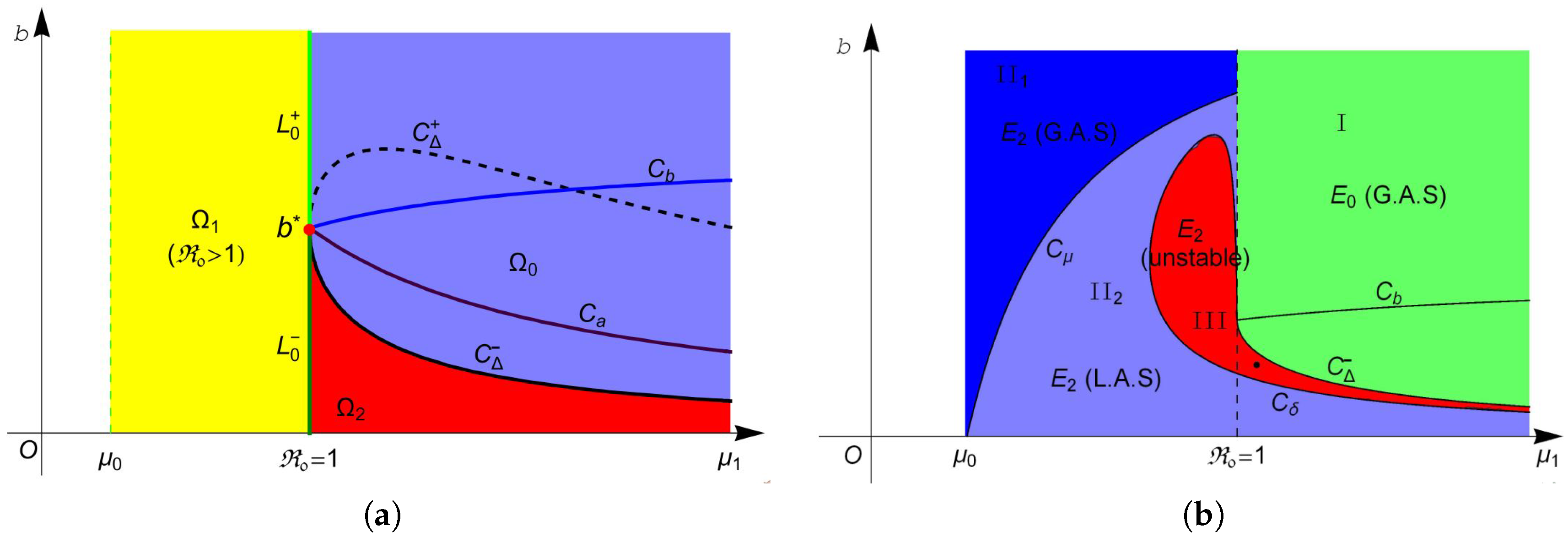
One can easily verify that hyperbola $C_a$ and line $L_0$ intersects at point $b^{*}=(\frac{\beta A}{d}-d-ϵ,\frac{d^2({\mu }_1-{\mu }_0)}{\beta A(\beta +\alpha d)})$, and $f_a({\mu }_1)$ is a decreasing convex function of ${\mu }_1$ with a horizontal asymptote $b=0$.

If ${\Delta }_0({\mu }_1,b)=0$, we obtain the curves $C_{\Delta }^{\pm }$ by solving b in term of ${\mu }_1$, where

$$C_{\Delta }^{\pm }:b=\frac{\beta A({\mu }_1-{\mu }_0)+{\delta }_0(d{\delta }_1-\beta A)\pm 2\sqrt{\beta ({\mu }_1-{\mu }_0){\delta }_0(d{\delta }_1-\beta A)}}{(\beta +\alpha d){\delta }_1^2}\triangleq f_{\Delta }^{\pm }({\mu }_1).$$

A straightforward calculation leads to $f_{\Delta }^{\pm }(\frac{\beta A}{d}-d-ϵ)=\frac{d^2({\mu }_1-{\mu }_0)}{\beta A(\beta +\alpha d)}$ and $f_{\Delta }^{\prime \pm }(\frac{\beta A}{d}-d-ϵ)=\pm \infty$, which suggests that $C_{\Delta }^{\pm }$ is tangent to the curve $L_0$ at the point $b^{*}$. Furthermore, for any ${\mu }_1\in (\frac{\beta A}{d}-d-ϵ,+\infty )$, we have

$$f_{\Delta }^{-}({\mu }_1)<f_a({\mu }_1)<f_{\Delta }^{+}({\mu }_1)$$

and

$$\frac{d{f}_{\Delta }^{-}({\mu }_1)}{d{\mu }_1}<0,\frac{d^2{f}_{\Delta }^{-}({\mu }_1)}{d{\mu }_1^2}>0,\underset{{\mu }_1\to +\infty }{lim}{f}_{\Delta }^{-}({\mu }_1)=0.$$

Therefore, the curve $C_{\Delta }^{-}$ under the curve $C_a$ is convex and decreasing with the asymptote $b=0$. $\delta ({\mu }_1,b)=0$ determines a curve $C_{\delta }$

$$C_{\delta }:\frac{-a_1+\sqrt{{\Delta }_0}}{2a_0}{m}_1+m_2\triangleq f_{\delta }({\mu }_1,b),$$

where $m_1,m_2$ are given in (23). Furthermore, we define

$$\begin{array}{c}{\displaystyle C_b:b=\frac{d({\mu }_1-{\mu }_0)}{(\beta +\alpha d)(d+ϵ+{\mu }_1)},C_{\mu }:b=\frac{{\mu }_1-{\mu }_0-2d}{\beta +\alpha d+\alpha {\delta }_1},}\hfill \end{array}$$

which will be used later.

Based on the above discussions and Theorem 1, let

$$\begin{array}{c}{\Omega }_0=\left\{({\mu }_1,b)|b>f_{\Delta }^{-}({\mu }_1),{\mu }_1>\beta A/d-d-ϵ\right\},\hfill \\ {\Omega }_1=\left\{({\mu }_1,b)|b>0,{\mu }_0<{\mu }_1<\beta A/d-d-ϵ\right\},\hfill \\ {\Omega }_2=\left\{({\mu }_1,b)|0<b<f_{\Delta }^{-}({\mu }_1),{\mu }_1>\beta A/d-d-ϵ\right\}.\hfill \end{array}$$

Then, system (4) has no endemic equilibrium in region ${\Omega }_0$, one endemic equilibrium $E_2$ in region ${\Omega }_1$ and two equilibria $E_1$ and $E_2$ in region ${\Omega }_2$. The two equilibria in ${\Omega }_2$ coalesce into one equilibrium $E^{*}$ on curve $C_{\Delta }^{-}$. For more intuitive observation, one can see Figure 1a.

Figure 1. (a) the bifurcation curve in the $({\mu }_1,b)$ plane; and (b) the stability curve of equilibria in the $({\mu }_1,b)$ plane.

The stability of these equilibria can be observed in Figure 1b. According to Theorem 2, the disease-free equilibrium $E_0$ always exists, and it is locally asymptotically stable (L.A.S) in region ${\Omega }_0\cup {\Omega }_2$ and unstable in region ${\Omega }_1$. Furthermore, Theorem 4 suggests that $E_0$ is globally asymptotically stable (G.A.S) in region I (green region in Figure 1b). From Theorem 3, we know that $E_1$ is always unstable whenever it exists, and $E_2$ is unstable in region II (red region in Figure 1b) and is L.A.S. in region II${}_1$ (light blue region in Figure 1b). 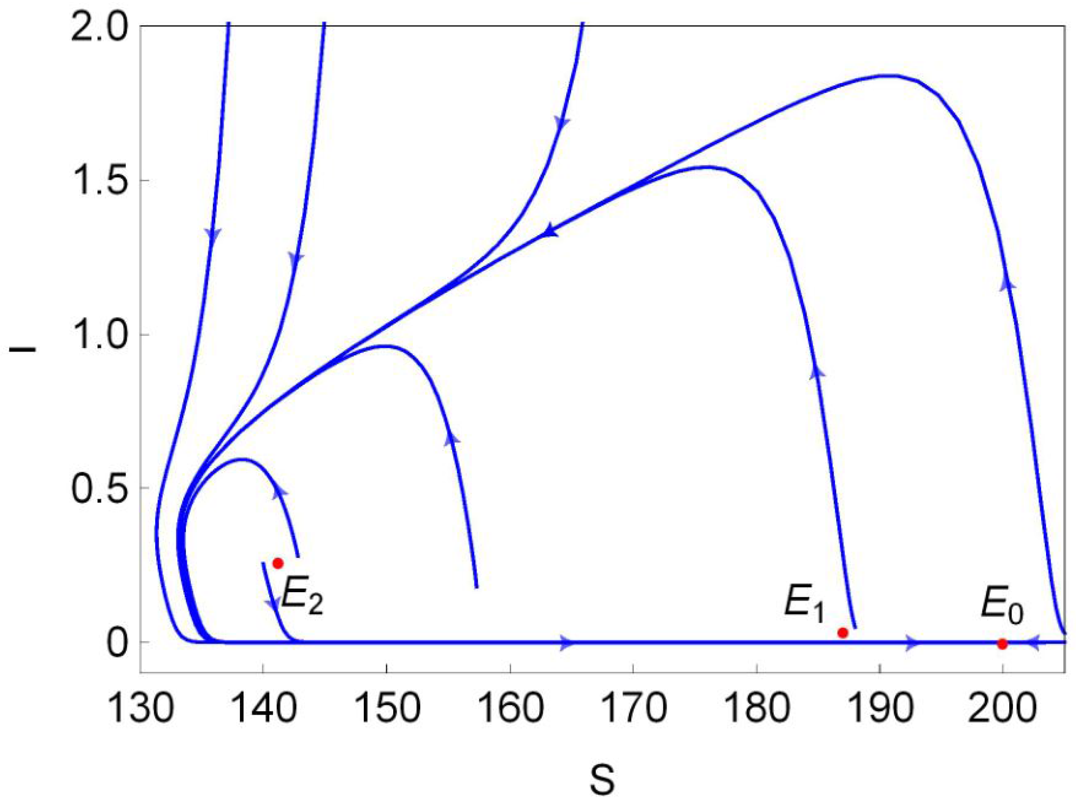Moreover, Theorem 4 implies that $E_2$ is G.A.S in region II${}_2$ (blue region in Figure 1b). Finally, we choose a point (marked in black dot in Figure 1b) in the region III and plot its phase portrait in Figure 2. It is clear that the disease-free equilibrium $E_0$ and two endemic equilibria $E_1$ and $E_2$ coexist, and $E_0$ is L.A.S, $E_1$ is a saddle and $E_2$ is unstable.

Figure 2. Phase portrait of system (4) when $E_0$, $E_1$ and $E_2$ coexist. Here, $A=20,\beta =0.2,d=0.1,\alpha =1,ϵ$ = 1, $b=0.15$, ${\mu }_1=41$ and ${\mu }_0=10$.

According to Theorem 5, system (4) undergoes forward bifurcation on $L_0^{+}$, backward bifurcation on $L_0^{-}$, pitchfork bifurcation when transversally passing through the line $L_0$ at point $b^{*}$ and saddle-node (SN) bifurcation on the curve $C_{\Delta }^{-}$ when the two endemic equilibria coalesce into one endemic equilibrium $E^{*}$. Hopf bifurcation occurs on the curve $C_{\delta }$ as proved in Theorem 7. 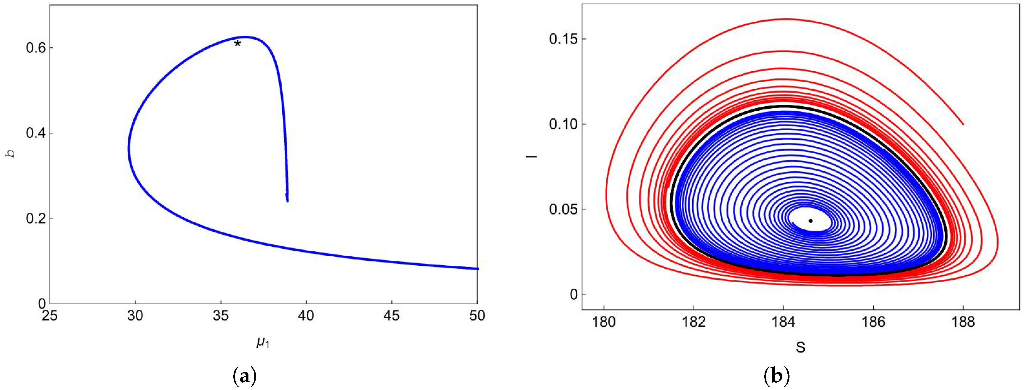Figure 3a shows the Hopf bifurcation curve in the ${\mu }_1-b$ plane. We choose one point $({\mu }_1,b)=(36,0.615)$ marked with a black asterisk below the blue curve in Figure 3a, and plot the phase portrait at this point in Figure 3b. We can observe from Figure 3b that the trajectory (blue curve) starting at $(184.2,0.042)$ spirals outward to the stable limit curve (black curve) and the trajectory (red curve) starting at $(188,0.1)$ spirals inward to the stable limit curve. At point $({\mu }_1,b)=(36,0.615)$, one can easily obtain that $E_1$ does not exist and $E_2$ exists, but it is unstable. Therefore, system (4) has a stable limit curve that enriches the unstable equilibrium $E_2$.

Figure 3. (a) Hopf bifurcation curve in ${\mu }_1-b$ plane. The black asterisk below the curve is the point we choose to plot the portrait in (b). Here, other parameters have the same values as in Figure 2.

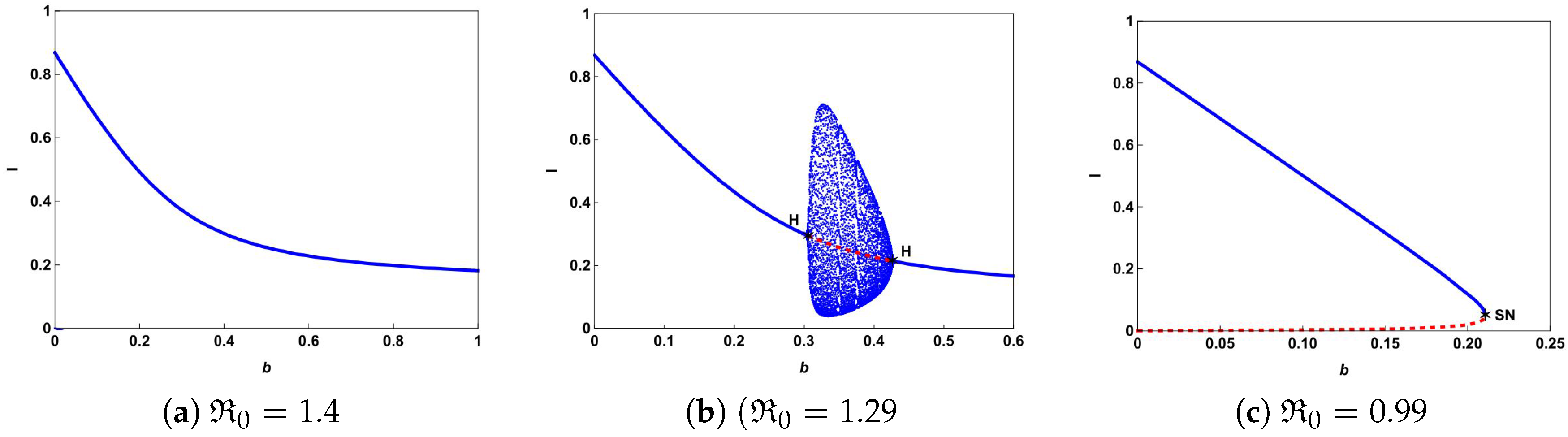
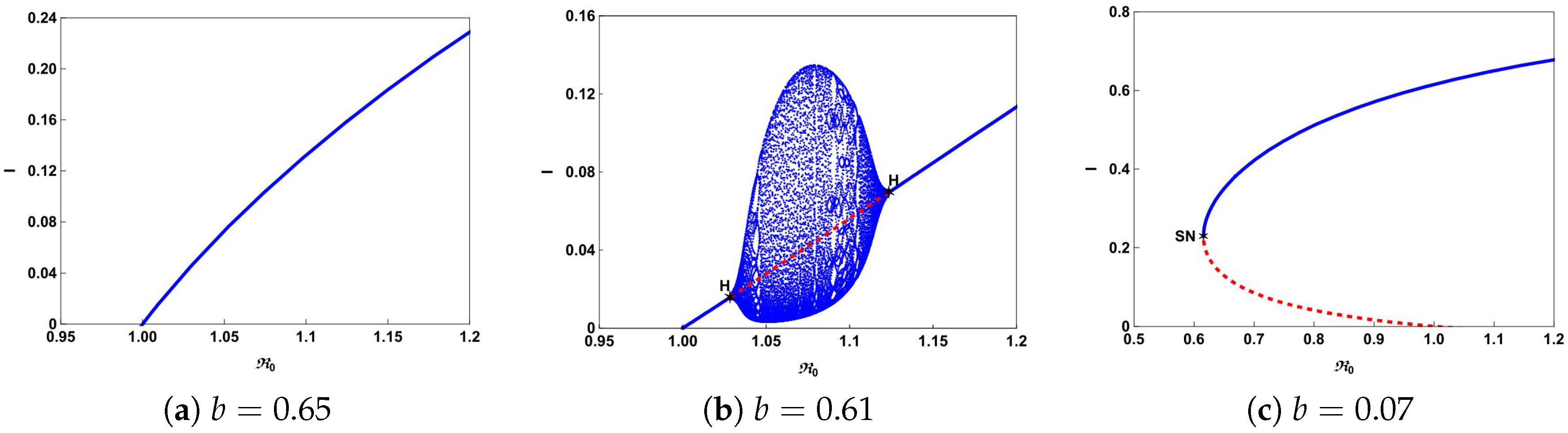
The typical bifurcation diagrams in ${\mathfrak{R}}_0-I$ plane can be seen in Figure 4. Figure 4a shows that there is a forward bifurcation at ${\mathfrak{R}}_0=1$ from disease-free equilibrium $E_0$ to a unique endemic equilibrium $E_2$ when ${\mathfrak{R}}_0>1$. If we decrease b from 0.65 to 0.61, system (4) not only undergoes forward bifurcation but also undergoes Hopf bifurcation as shown in Figure 4b. In this case, a stable limit cycle bifurcated from forward Hopf bifurcation and disappears from the backward Hopf bifurcation. If we further decrease b to 0.07, we can observe from Figure 4c that the backward bifurcation and saddle-node bifurcation occur. This illustrates that the number of hospital beds plays an important role in controlling an infectious disease.

Figure 4. Bifurcation diagrams of system (4) in ${\mathfrak{R}}_0-I$ plane with different b. The blue curves represent the stable fix points or limit cycles and the red dashed curves represent the unstable fix points.

To further explore the impact of the number of hospital beds, we also present the possible bifurcation diagrams in $b-I$ plane by fixing all the parameters except b. Figure 5 depicts some typical bifurcation diagrams in $b-I$ plane with different ${\mathfrak{R}}_0$. If ${\mathfrak{R}}_0>1$, one can see from Figure 5a,b that increasing the beds can reduce the number of infectious individuals but can not eliminate the disease. Especially in the case of ${\mathfrak{R}}_0=1.29$, Hopf bifurcation occurs and a stable limit cycle bifurcated from forward Hopf bifurcation disappears from backward bifurcation. If ${\mathfrak{R}}_0<1$, backward bifurcation and saddle-node bifurcation may occur and the disease dies out when the value of b is above the curve $C_{\Delta }^{-}$ based on Theorem 4 and Figure 1.

Figure 5. Bifurcation diagrams of system (4) in $b-I$ with different ${\mathfrak{R}}_0$.

Finally, we investigate the effect of the nonlinear incidence rate. For the nonlinear saturate incidence rate $\beta SI/(1+\alpha I)$, it is known that larger $\alpha$ reflects stronger inhibition effect caused by the infective individuals. Although the increasing of $\alpha$ cannot reduce the basic reproduction number ${\mathfrak{R}}_0$, it does affect the dynamical behaviors of the system. 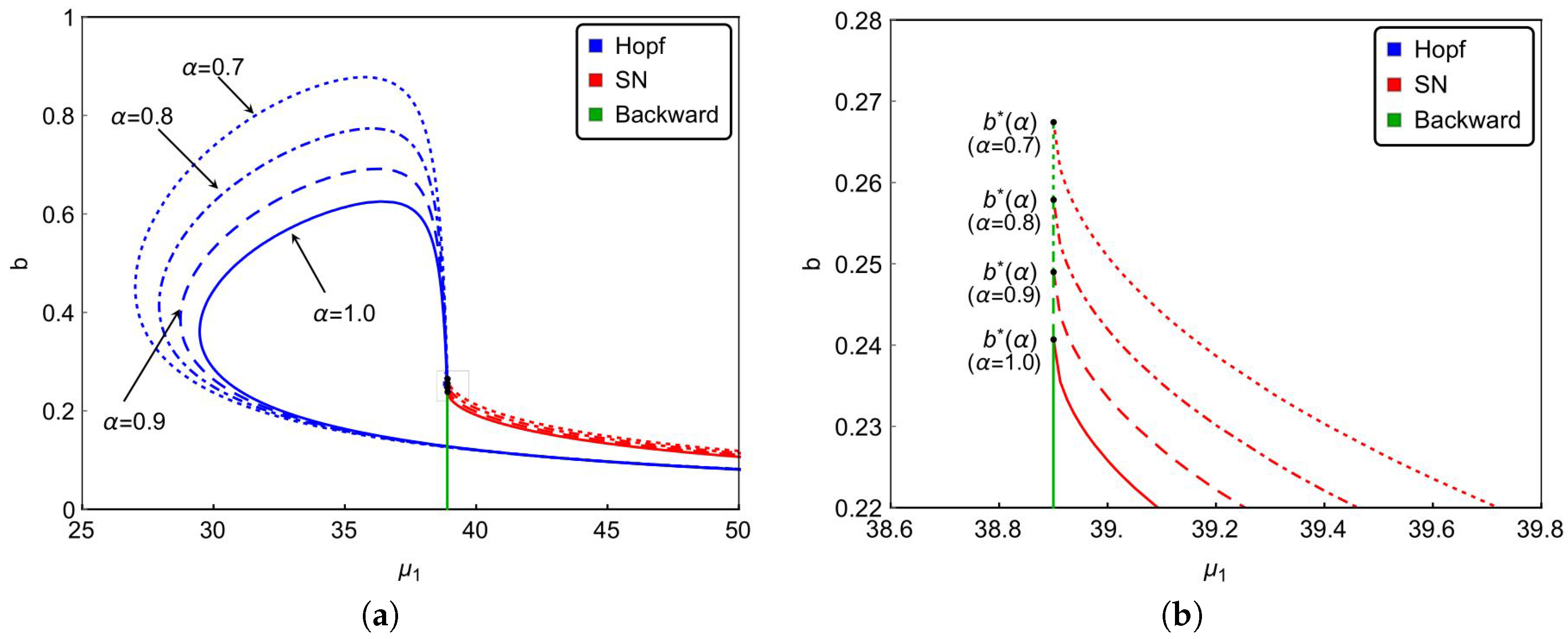Based on previous results, we can see from Figure 6a that backward bifurcation occurs on green lines, saddle-node bifurcation occurs on red curves and Hopf bifurcation happens on blue curves. Figure 6a and the magnified diagram Figure 6b also illustrate that the occurrence of backward bifurcation, saddle-node bifurcation and Hopf bifurcation shrink with increasing $\alpha$. That is to say, the strong inhibition effect will lower the complexity of the transmission of the infectious diseases. In other words, enhancing the public’s defensive “crowding effect” through education or medium is beneficial to control and prevent the spread of the infectious diseases. Furthermore, Figure 6 also implies that the stronger inhibition effect of the lower number of hospital beds will be needed to eliminate the diseases. It reveals that strengthened public defensive “crowding effect” can mitigate the demand for hospital beds in controlling the spread of the disease during an outbreak.

Figure 6. (a) impact of the nonlinear incidence rate on dynamical behaviors of system (3); (b) the magnified diagram of black box marked in figure (a). Besides $\alpha$, other parameters have the same values as in Figure 2.

5. Discussion

Due to the important biological significance of hospital beds, in this paper, we have investigated an SIR epidemic model to simulate the impact of a limited health care system in terms of the number of hospital beds. Theoretical analysis and numerical simulations illustrated that system (4) has at most three equilibria and possesses complex nonlinear dynamics. From Theorems 5–7 and Figure 4 and Figure 5, we have shown that system (4) can undergo backward bifurcation, saddle-node bifurcation and Hopf bifurcation due to the insufficient number of hospital beds.

If ${\mathfrak{R}}_0>1$, it follows from Theorem 3 and Figure 1b that $E_2$ is the unique endemic equilibrium, and it is stable if b is sufficiently large such that the values of b are all above the curve $C_{\delta }$. Since $I_2>0$ and $\frac{\partial I_2(b)}{\partial b}{|}_{b>0}<0$, then $I_2(b)$ is a monotone decreasing function of b and $I_2(b)$ trends to some positive constant as b to infinity. That is, increasing the number of hospital beds can only reduce the number of the infectious, but cannot eliminate the infectious disease (see Figure 5a,b). If ${\mathfrak{R}}_0<1$, it follows from Theorem 3 and Figure 1b that the disease can be eliminated when the value of b above the curve is $C_{\Delta }^{-}$. This means that the basic reproduction number is not the only evaluation standard for the control and elimination of the disease. It also depends on the resources of the health care system such as the number of hospital beds.

The bifurcation analysis is carried out through reducing the three dimension model (3) to the planar system (4). The typical bifurcation curves and diagrams are shown in Section 4, and all of the results reveal that system (3) possesses complex dynamics such as forward bifurcation, backward bifurcation, saddle-node bifurcation and Hopf bifurcation. Contrasting to the results for the classic SIR epidemic models, we also find that the nonlinearity of incidence rate and recovery rate are important factors that lead to very rich dynamics. Moreover, we find that the dynamical behavior of system (3) not only depends on ${\mathfrak{R}}_0$ but also relies on the number of hospital beds and the inhibition effect caused by the infective individuals. Therefore, the public health makers should consider the combined effects of the government intervention strategies (such as education and medium) and hospitalization conditions to make guidelines in controlling the spread of infectious diseases. Hopefully, in the future, we can explore more theoretical results to control and eliminate infectious diseases, especially in the outbreak of diseases.

References

- Anderson, R.M.; May, R.M. Infectious Diseases of Humans: Dynamics and Control; Oxford University Press: New York, NY, USA, 1991. [Google Scholar]
- Brauer, F.; Castillo-Chávez, C. Mathematical Models in Population Biology and Epidemiology; Springer: New York, NY, USA, 2001. [Google Scholar]
- Diekmann, O.; Heesterbeek, J.A.P. Mathematical Epidemiology of Infectious Diseases: Model Building, Analysis and Interpretation; John Wiley & Sons Ltd.: New York, NY, USA, 2000. [Google Scholar]
- Hethcote, H.W. The mathematics of infectious disease. SIAM Rev. 2000, 42, 599–653. [Google Scholar] [CrossRef]
- Liu, W.; Hetchote, H.W.; Levin, S. Influence of nonlinear incidence rates upon the behavior of SIRS epidemiological model. J. Math. Biol. 1986, 23, 187–204. [Google Scholar] [CrossRef] [PubMed]
- Ruan, S.; Wang, W. Dynamical behavior of an epidemic model with a nonlinear incidence rate. J. Differ. Equ. 2003, 188, 135–163. [Google Scholar] [CrossRef]
- Tang, Y.; Huang, D.; Ruan, S.; Zhang, W. Coexistence of limit cycles and homoclinic loops in a SIRS model with a nonlinear incidence rate. SIAM J. Appl. Math. 2008, 69, 621–639. [Google Scholar] [CrossRef]
- Capasso, V.; Serio, G. A generalization of the Kermack-McKendrick deterministic epidemic model. Math. Biosci. 1978, 42, 43–61. [Google Scholar]
- Hu, Z.; Ma, W.; Ruan, S. Analysis of SIR epidemic models with nonlinear incidence rate and treatment. Math. Biosci. 2012, 238, 12–20. [Google Scholar] [CrossRef] [PubMed]
- Liu, R.; Wu, J.; Zhu, H. Media/psychological impact on multiple outbreaks of emerging infectious diseases. Comput. Math. Methods Med. 2007, 8, 153–164. [Google Scholar] [CrossRef]
- Wang, W. Backward bifurcation of an epidemic model with treatment. Math. Biosci. 2006, 201, 58–71. [Google Scholar] [CrossRef] [PubMed]
- Zhou, L.; Fan, M. Dynamics of an SIR epidemic model with limited medical resources revisited. Nonlinear Anal. Real World Appl. 2012, 13, 312–324. [Google Scholar] [CrossRef]
- Shan, C.; Zhu, H. Bifurcations and complex dynamics of an SIR model with the impact of the number of hospital beds. J. Differ. Equ. 2014, 257, 1662–1688. [Google Scholar] [CrossRef]
- Wang, W.; Ruan, S. Simulating the SARS outbreak in Beijing with limited data. J. Theor. Biol. 2004, 227, 369–379. [Google Scholar] [CrossRef] [PubMed]
- World Health Statistics 2005–2014. Available online: http://www.who.int/gho/publications/world_health_statistics/en/ (accessed on 22 June 2017).
- Abdelrazec, A.; Bélair, J.; Shan, C.; Zhu, H. Modeling the spread and control of dengue with limited public health resources. Math. Biosci. 2016, 271, 136–145. [Google Scholar] [CrossRef] [PubMed]
- Casabán, M.-C.; Cortés, J.-C.; Navarro-Quiles, A.; Romero, J.-V.; Roselló, M.-D.; Villanueva, R.-J. A comprehensive probabilistic solution of random SIS-type epidemiological models using the random variable transformation technique. Commun. Nonlinear Sci. 2016, 32, 199–210. [Google Scholar] [CrossRef]
- Ji, C.; Jiang, D.; Shi, N. The behavior of an SIR epidemic model with stochastic perturbation. Stoch. Anal. Appl. 2012, 30, 755–773. [Google Scholar] [CrossRef]
- Van den Driessche, P.; Watmough, J. Reproduction numbers and sub-threshold endemic equilibria for compartmental models of disease transimission. Math. Biosci. 2002, 180, 29–48. [Google Scholar] [CrossRef]
- Wiggins, S. Introduction to Applied Nonlinear Dynamical Systems and Chaos, 2nd ed.; Texts in Applied Mathematics; Springer: New York, NY, USA, 2003; Volume 2. [Google Scholar]
- Guckenheimer, J.; Holmes, P.J. Nonlinear Oscillations, Dynamical Systems, and Bifurcation of Vector Fields; Springer: New York, NY, USA, 1983. [Google Scholar]
© 2017 by the authors. Licensee MDPI, Basel, Switzerland. This article is an open access article distributed under the terms and conditions of the Creative Commons Attribution (CC BY) license (http://creativecommons.org/licenses/by/4.0/).