Abstract
Here, we consider the following inverse problem: Determination of an increasing continuous function on an interval from the knowledge of the integrals where the are random variables taking values on and are given numbers. This is a linear integral equation with discrete data, which can be transformed into a generalized moment problem when is supposed to have a positive derivative, and it becomes a classical interpolation problem if the are deterministic. In some cases, e.g., in utility theory in economics, natural growth and convexity constraints are required on the function, which makes the inverse problem more interesting. Not only that, the data may be provided in intervals and/or measured up to an additive error. It is the purpose of this work to show how the standard method of maximum entropy, as well as the method of maximum entropy in the mean, provides an efficient method to deal with these problems.
1. Introduction
As stated above, in this work we are interested in applying maxentropic techniques to solve integral equations in which growth and convexity constraints may be imposed on the solution. In addition, we can suppose that the data may be given up to an interval and/or be contaminated with additive errors.
Since utility theory motivates and provides a natural setup for many of the questions that we are interested in, we shall recall some very basic definitions, and now and then use the name of utility for the function that we are determining by solving the system of integral equations.
Utility theory forms the basis of both the theoretical and applied analysis to understand the process of decision making under uncertainty (see Eeckhoudt et al. [1] and Luenberger [2] for an introduction to the subject, and also the paper by Herstein and Milnor [3], in which they show how to relate preferences to utility functions).
A utility function is an increasing, continuous function which is used by a decision maker to rank random payoffs modeled by random variable taking values in A decision maker who with utility function is confronted with the need to choose among a variety of risky ventures or bets with random payoff will prefer the bet that has the largest expected utility To model risk aversion or risk proneness, convexity constraints are imposed upon
An important concept which relates the determination of a utility function to an interpolation problem is that of the certainty equivalent. In its simplest form, it is the quantity which an investor is willing to accept instead of the outcome of a random bet, that is, it is the wealth that has the same utility as the expected utility of a random bet In other words, for a given it is the number such that:
In order to display the relationship of the different problems among themselves, we organize this section as follows. First, we shall explain how the integral equation can be regarded either as generalized moment problem or an interpolation problem, then explain how the problem is to be stated when the data is provided up to an interval or when there are measurement errors. After that we shall briefly review some of the methods that have been used to solve some of those problems, and close the section describing the remainder of the paper.
1.1. Problem Statements: The Certain Data Case
Generic problem statement
Determination of an increasing and continuous function having some specified convexity properties, such that the left hand side of:
is known for a finite collection of random variables taking values in , denote their cumulative distribution functions, and stands for the expected utility of each random bet
Problem 1 (The generalized moment problem).
An interesting twist on (1) is obtained if we suppose that is differentiable, except perhaps at a countable set of points and suppose that and are known. Then we can scale U in such a way that (using U again to denote the scaled function) and Then, a simple integration by parts shows that:
where is positive due to the fact that we are considering U to be increasing. Also Rewritten that way, (1) becomes a generalized moment problem consisting of determining the density from the knowledge of the generalized moments
When the certainty equivalents of the are known, we obtain a relationship between the generalized moment problem and an interpolation problem by setting:
where now is the indicator function of the interval and is a given collection of points. Therefore, for an appropriately scaled increasing and differentiable function, solving the integral equation system is related to a generalized moment problem and to an interpolation problem. Notice as well that if the in Equation (1) were certain, then (2) becomes the interpolation Problem (3).
Problem 2 (Interpolation problem).
A direct relationship between (1) and an interpolation problem comes up if we suppose that the certainty equivalent of the as well as their expected utilities are known. In this case (and at this stage we do not need differentiability assumptions on the function ) Problem (1) becomes: Determination of a continuous increasing function such that:
where the are supposed to be the results of the computation of the expected value in (1). So, for this choice of random bets, the interpolation Problems (3) and the moment Problem (1) are related, except that in the former case we search for U directly, whereas in the latter we search for We mention that the existence of the certainty equivalents is clear from the fact that U is continuous and increasing and that When considering the application to utility functions, the are supposed to be elicited from the investor or decision maker.
1.2. Problem Statements: The Uncertain Data Case
A first extension of (1) corresponds to the case in which the data is not a single number for each but an interval which contains the true number. The uncertainty may come from an uncertainty about the probability distribution of the or from the data collection process. To motivate from the point of view of utility theory, we may think that all that the decision maker is able to provide is a range for the utility of a given wealth.
Problem 3 (Expected values are uncertain).
Determination of an increasing and continuous function having some not yet specified smoothness or convexity properties, such that:
for a finite collection of random variables where the are given intervals.
Problem 4 (Interpolation with uncertain data).
When the are deterministic and concentrated at or when the certainty equivalents of the are known, we obtain an interpolation problem with uncertain data. The extended version of Problem 2 becomes: determination of a continuous, increasing function perhaps having some specified smoothness and convexity properties, such that:
the notation being as above. Again, observe that when the values and are known (or set equal to 0 and 1 by appropriate rescaling), and the function U is supposed to be differentiable, by transforming Problem (5) as in (2) it becomes a generalized moment problem with uncertain data.
1.3. Problem Statements: The Case of Errors in the Data
The interpretation of this setup is a bit different. In this case we suppose that we are given values for either the utility of some possible wealths or the expected utility of some random payoffs. However, it is known that the computation of the reported number involves approximations or round off errors. The statement of the problem to solve in this case, is similar to, yet different from the two cases considered above. Consider:
Problem 5 (Expected utility computed with errors).
Determination of an increasing and continuous function perhaps having some specified convexity properties, such that:
for a finite collection of random variables The numbers are known up to an additive error that has to be estimated as well. A model for the “measurement” error is available to the modeler.
Problem 6 (Utility function computed with errors).
Determination of a continuous and increasing function perhaps having some specified convexity properties, such that:
for a set of given numbers where, again, the are to be estimated as well. Also, a model for the “measurement” error is available to the modeler.
1.4. Comments about the Solutions to the Generalized Moment and Interpolation Problems
We begin by saying that solving Problem (3) by means of maxentropic methods is not new. The papers by Abbas [4,5,6] where it seems to have been applied for the first time, and later on Abbas (2006), Darooneh [7], Pires et al. [8] and Pires et al. [9], describe different maxentropic approaches to the problems and contain references to previous work on the specific applications to utility theory. Actually, the transformation of problems (1) into (2) was considered in Abbas’ papers. But none of these papers considers the case of data up to an interval or the case of errors in the data. In this regard we mention the work by Abbas [10]. Referring to the finite dimensional version of (1), he considers the possibility of prescribing ranges for the utility function or for the probability distributions to be determined.
There are many ways of solving interpolation problems like (4), from linear spline interpolation to polynomial interpolation. For interpolation methods in which convexity is a constraint, consider Mettke [11], Lai [12] and Visnawathan et al. [13]. Besides that, there is the parametric approach, which assumes that U has a known form, with shape and scale parameters that are to be fitted by lest squares. See Luenberger [2] for this approach.
We should mention that the direct maxentropic solution to Problem (3) leads to a piecewise constant which in turn leads to a piecewise linear reconstruction of
Let us mention that there is another interesting type of problem, which in some sense is a dynamic version of the problem that we consider here. Instead of prescribing the expected values of a few random variables, one may prescribe a curve solving some optimality criterion, and then obtain a differential equation for In utility theory, this corresponds to determining a utility function given an optimal investment and consumption policy of an agent during a certain time period. Consider for example, Dybvig and Rogers [14] or Cox, Hobson and Obłój [15] and the references cited therein. The application of the standard maxentropic methods to economics and finance is anything but new. Consider the papers by Buchen and Kelly [16], Stutzer [17], Gulko [18] and see the review by Zhong et al. [19] for much more.
Originally, the standard method of maximum entropy was proposed in Jaynes [20] to solve problems such as (3). This method admits extensions to deal with the cases of data in intervals or errors in the data (see for example Gomes-Gonçalves et al. [21]). However, the method also admits another extension to deal with problems like (1) in which the unknown is not a density, but a function which may have any sign and not necessarily integrate to Such extension seems to have been originally proposed in Navaza [22], the mathematics of which were developed by Dacunha-Castelle and Gamboa [23]. The method of maximum entropy in the mean has made its way into econometrics. See Golan et al. [24] for a review cf previous work and applications, Golan and Gzyl [25] for a unification of notation, and Gzyl and Velásquez [26] for detailed development. For applications to problems such as (1), (5), (7), see Gzyl and Mayoral [27,28]. To conclude the short digression about maximum entropy on the mean, we mention here that it is much more general and flexible than the standard method of maximum entropy, and contains a particular case (see Gzyl and ter Horst [29]). Such extension is a good tool for solving problems such as (3), (6), (8).
1.5. The Organization of the Paper
Having described the various versions of an integral equations problem to determine a function U that has to satisfy some collateral conditions, as well as two possible extensions of the problem, we mention here that the aim of this work is to present a method that solves all of these problems as variations on the theme of a single technique based on the method of maximum entropy.
The remainder of the paper is organized as follows: In Section 2 we shall see how to transform the integral equation problem for into an integral equation for This covers the case in which the original function is required to be convex or concave. This requirement determines a signature constraint imposed on As the integral equation (for ) has to be solved numerically, in a short Section 3 we show how to discretize the integral equation problem in order to apply the method of maximum entropy in the mean to solve this case.
In Section 4 we collect the basics results on the different variations and extensions of the maximum entropy method. We begin with the standard method of maximum entropy which is a stepping stone for the method of maximum entropy in the mean, end then explain this last method.
Section 5 is devoted to numerical examples built upon the examples considered by Abbas (2006) and Luenberger (1998). These were chosen as representative of the two different approaches (that is, regarding the interpolation problem as a generalized moment problem or an interpolation problem). To consider extensions, in each case we either add noise to the data or consider that the data is given up to some small interval about the original data. We modify the data that they provided to examine the different possible variations on the theme. We close with a few final comments.
2. Incorporation of Convexity Constraints
Suppose that is differentiable twice, with a bounded, measurable derivative. A simple integration by parts yields the identity:
This transforms the interpolation problem into an integral equation. At this point, we mention that even though the knowledge of the values and may be assumed in applications, the value of has to be estimated.
If the function U is required to be concave, a lower bound is easy to obtain. Since for is above the line joining to clearly However, at the end, either its value or a range for it, has to be supplied by the modeler. We mention as well that the uncertainty in the specification of the derivative introduces an uncertainty in the specification of the datum that we call m a few lines below, which leads us to a problem with data in intervals or a problem with errors in the data.
Observe as well that, if is required to be convex, then has to be positive, whereas if is to be concave, then must be negative. To be specific, with applications to utility theory in mind, we shall consider the risk- averse decision maker and require to be positive. To simplify the notation, shall write and recast Problem (3) as: finding a positive function such that:
where Note that the right hand side of this identity is positive. Coming back to the statement of Problem 1, note that under the same conditions on U mentioned above, substituting in (2) and using de fact that we obtain after exchanging integrals:
Again, note that when is certain, say for some then and Thus the interpolation problem with convexity constraints becomes an integral equation problem like:
in which the specification of the data depends not only on but on as well.
To make all these problems look formally alike, write and rewrite (9) as:
and when the data is uncertain, we would need to solve:
Clearly, all the problems described in Section 1 lead to our wanting to solve the same generalized moment problems like (12) and (13), with boundedness constraints imposed on the solution.
3. Discretization of the Problems
Since we want to solve the problems numerically, we must discretize the integral equations introduced in the previous sections. Let us describe the generic problem: Determine a continuous function (or ) that satisfies:
Notice that when for we are reduced to case of solving a standard generalized moment problem. Denote by with the left end points of a partition of into N sub-intervals. Define the vector to have components Define the matrix A by its components constructed from the datum as:
Define to be the data region and (or ) to be the constraint set, that is the set in which the solution to the discretized problem has to lie. With this notation, the discrete version of Problem (14) becomes:
which is a standard linear inverse problem with (non-linear) convex constraints. As said, the method of maximum entropy in the mean handles such problems in a systematic fashion.
4. The Maximum Entropy Methods
The results presented below are not new, and are included for completeness. It may be skipped by readers familiar with the methodology. The complete proofs of the statements about convex duality are provided in Borwein and Lewis [30] and in Gzyl and Velásquez [26].
This section is divided into three subsections. In the first one we review the standard method of maximum entropy (SME), then the second its extension (SMEE) to incorporate uncertain data. As we explained, these will be applied to the first two problems and to their extension when the data is uncertain or has errors. Then we review the method of maximum entropy in the mean (MEM) and its extension to the case of uncertain data. We shall apply this technique to the case in which one wants to determine the second derivative of U from the data about preferences.
4.1. The Standard Maximum Entropy Method (SME)
The standard maximum entropy method (SME) is the name of a variational procedure to solve the (inverse) problem consisting of finding a probability density (on ) in our case, satisfying the following integral constraints:
The notation follows that introduced during the generic statement of Problems 1 to 6. The material presented below is standard, and here we recall the results that we use for the numerical computations. We set and since we require to be a density function. It actually takes a standard computation to see that when the problem has a solution it is of the type:
in which the number of moments M appears explicitly. It is usually customary to write where is an -dimensional vector. Clearly, the generic form of the normalization factor is given by:
With this notation the generic form of the solution can be rewritten as:
The vector can is found minimizing the dual entropy:
where denotes the standard Euclidean scalar product and m is the -vector with components and obviously, the dependence of on m is through A simple calculation shows the first order condition for to be a minimizer of which is equivalent to saying that (19) satisfies (16).
4.2. The Standard Maximum Entropy for Data in Ranges (SMEE)
Here we present an extension of the method described above to solve the (inverse) problem consisting of finding a probability density (on in this case), satisfying the following integral constraints:
where the interval around the true but unknown depends on the undecided decision maker. For only we set since for we have to take care of the natural normalization requirement on
Let us put The idea behind the SMEE is to solve a SME problem for each , and then maximize over the entropy of these solutions. That eventually leads to the need of minimization of the following dual entropy function:
where:
is the Fenchel–Legendre dual of the indicator of the convex set (see Borwein and Lewis (2000) for these matters). To obtain this result, just notice that can be mapped onto by means of affine mapping, and:
As a first step towards describing the solution, we state the following result, the proof of which can be seen in Borwein and Lewis [30].
Lemma 1.
With the notations introduced above, set
Then is strictly convex in
If the minimum of is reached at a point in the interior of the set then maxentropic solution to the inverse problem (21) is given by:
Since the numerical minimization of is necessary for the determination of the optimal the following computation is worth keeping in mind. Observe that is defined except at where it is sub-differentiable (see Borwein and Lewis (2000)). Actually,
Keeping the above computations in mind, it is easy to verify that the first order condition for to be a minimizer yields.
4.3. The Method of Maximum Entropy in the Mean
In this section we come back to the problem of finding an increasing, continuous function with given boundary behavior and specified convexity constraints. Even though the method that we shall implement can take care of constraints like for given functions and we shall content ourselves with one of two possible cases: for some finite B or the case corresponding to the cases in which the second derivative of U is known to be bounded or not.
Recall that to solve the discrete version of Problem (15) we need to solve the linear system:
where will be either or and Let us explain how to solve it using MEM.
4.3.1. The Intuition Behind MEM
Maximum entropy in the mean is the name of a technique which allows us to transform an algebraic problem into a non-linear optimization problem of smaller dimension. The standard presentation of the method is explained in Gzyl and Velásquez [26]. Let us devote a few lines to explain the intuition behind it.
Instead of solving (15) we search for a probability P on where denotes the Borel algebra of subsets of such that solves (15), that is Here is the identity (or coordinate) map on To find P one proposes any interesting reference finite measure or probability Q, such that the closure of the convex hull of its support is and then one uses a maxentropic procedure to determine a positive density of P with respect to Q, such that:
It only remains to be added that it is by finding satisfying (24) that one solves a maximum entropy problem for each and then “best” density is determined as the one that maximizes the corresponding entropies.
4.3.2. MEM for the Problem with Preassigned Bounds
This part covers both the initial step for MEM with certain data as well as MEM for the problem with uncertain data. There are two cases to consider, depending on whether we want the unknown function to have preassigned bounds or not. The procedure is the same, but the constraint space is not.
Case 1:
This is certainly the simple possible case, but it contains all the ingredients for the most general case. As any point in can be written as a convex combination of 0 and we choose as reference measure on the measure:
where denotes the unit point mass (Dirac’s measure) at B in the −th direction. Since any may be written as:
the constraint Equation (24) become:
where is any point. To find the ’s we introduce the usual entropy:
The standard argument leads to the representation:
where the identification in the last step can be read from (25). The normalization factor is given by:
and finally, the are to be found minimizing the dual entropy function:
Case 2: No bounds preassigned
This time and the rest of the notation has the same meaning as in the first case. A possible candidate for reference measure is a product of Poisson measures (of parameter ). This is so because they are supported by the non-negative integers and any point in the line can be obtained by a convex combination of integers. So, we consider:
If we denote by the density of the unknown measure P with respect to the constraint equations look like:
Now we have to maximize:
subject to (27), plus the normalization condition. The standard argument leads to the representation:
This time the normalization factor is easily computed to be:
The vector is found, minimizing:
The representation mentioned in the right hand side of (28) appears when we apply the first order condition for to be a minimizer of
4.4. Maximum Entropy in the Mean for the Case with Uncertain Data
Let us now address the problem of determining the utility function with prescribed convexity properties, when the utility function of the decision maker is known up to a range of values. We know that this problem reduces to the problem of determining such that:
The rationale to solve this problem is similar to that used in the SME with uncertain data: Solve a MEM problem for each and then maximize over the entropies of the resulting maxentropic densities.
That leads to the need to determine the minimizer of the dual entropy:
over We thus obtain a maxentropic density of over such that the mean:
is the solution to To go beyond these generalities, we must specify and
4.4.1. MEM for the Problem with Uncertain Data and Preassigned Bound on the Second Derivative
We consider the same two cases as before, according to whether the second derivative is bounded or not, but in both cases it is required to be positive. In both cases the set up and the arguments are similar to those used in Section 4.2 for the SME method when the data is uncertain. The representation of the density and the normalization factor are the same. All that changes is the dual function to be minimized to determine the optimal which this time is:
where the specification of the domain is chosen according the un-decidedness of the decision maker.
Case 1:
In this case the normalization factor found above is:
Therefore, now we have to find the minimizer of:
Also, once the optimal is found, the maxenntropic solution to our problem is:
Note that the solution looks similar that of the case in which the data is certain, except that this time the dual entropy is different. Note as well that when the two solutions to the two problems become identical.
Case 2: Positive
As said, the setup described in Section 4.2 can be transported verbatim. The normalization factor for this case is:
and therefore, to determine the optimal the function to be minimized in this case is:
This time, once the minimizer has been found, the maxentropic solution to the problem of determining the solution to (15) is:
4.5. Case with Errors in the Data and Uncertainty in the Data
This case extends Problem 6, and it was motivated by the following considerations. Notice that in the statement of (9), on one hand, the value of may only be known up to an interval, and on the other, when transforming the problem into an integral equation for the second derivative of U, and error may be introduced in the estimate of
Thus we are led to extend the statement of (24) to:
in which is a vector whose components lie in intervals containing the data points The uncertainty in the values of the function U and the capture the uncertainty due to errors in the estimation of say. Stated this way, the problem clearly extends the statement of Problem 6, in which the decision maker may be certain about his choice, but he misestimates the
To solve this problem the intuition about MEM carries on to this case. All we have to add is that we also want to think of the as expected values with respect to an probability law that must also be determined.
So as not to introduce much more symbols, denote by where I is the identity matrix and To simplify our lives we introduce that is, we suppose that all errors have the same bound.
Now, (15) becomes:
Note that when reduces to a point, we are back in the case of Problem 6. Again, the first step of the routine consists of choosing a measure on to play the role of reference measure. We shall chose a product measure (think of the subscripts as “signal” and “noise”). The is as above and for the noise we choose:
The Laplace transform of this measure is:
To define we replace by The density that maximizes the entropy is, again, given by:
where is obtained maximizing the dual entropy:
Bringing in the expression for the last identity becomes:
Once the that minimizes (33) has been determined, the representation of the (discretized) second derivative is given by an expression similar to (30), namely:
Also, the estimated errors are given by:
5. Numerical Examples
We shall consider extended versions of the numerical problems treated by Abbas and by Luenberger. The extensions go beyond the examples in two ways: First, we include the possibility that the data is known up to a range, and second, we include convexity constraints upon the unknown.
5.1. Abbas’ Example with and without Uncertainty
In Abbas (2006), the author uses the data in Table 1 and Problem (1) to determine regarded as a probability density on The scaling that he uses comes in handy for that interpretation. The first row in Table 1 contains a few possible wealths and in the second row we display the utility of that wealth. In the last row we list possible ranges of utility for the undecided decision maker.

Table 1.
Extended Abbas’ data.
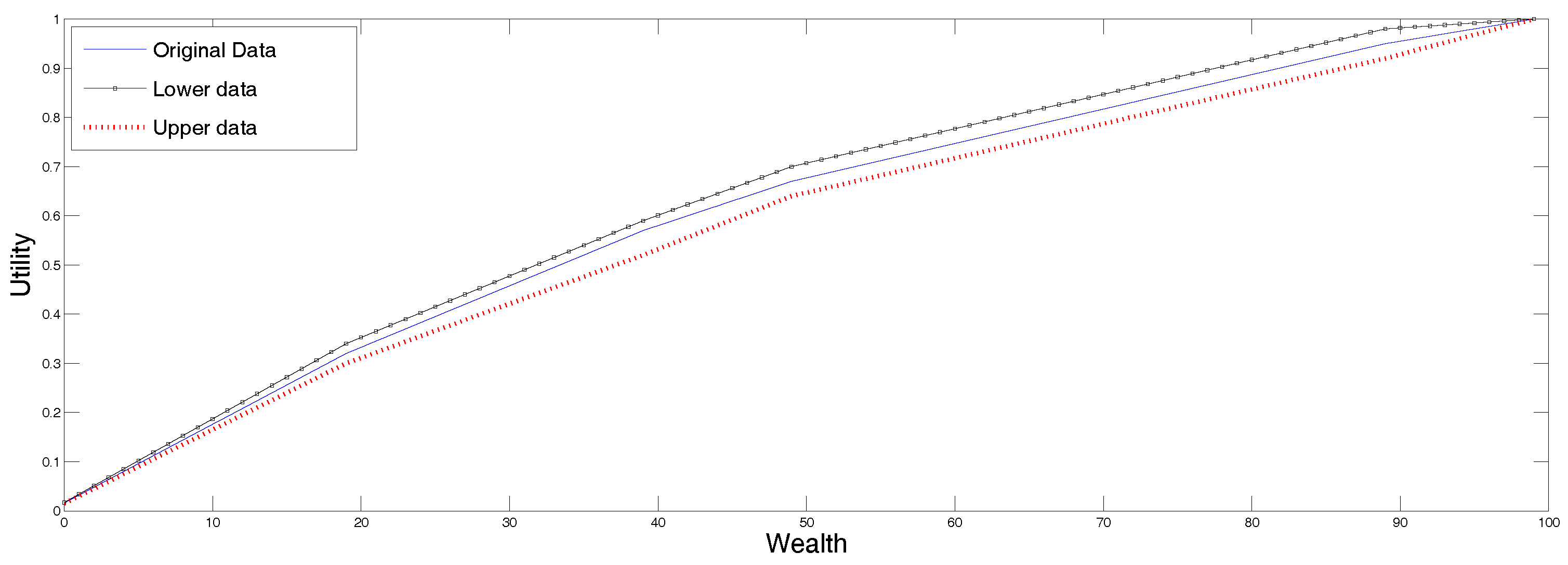
In Figure 1 we display following three possible reconstructions, all using the SME method. In the continuous line we present the reconstruction corresponding to the original data. The upper curve corresponds to the reconstruction using as inputs the upper ends points of the undecidability region, and the lower curve displays the utility corresponding to the lower end points of the undecidability region. The ordering of the utility functions is intuitively clear. This is because this approach uses the data in the third row in a trivial way, and since the utility function is increasing and interpolates a sequence of point values, the larger the values, the larger the interpolated function. Therefore, any other method using the interval data, must produce a result within those two graphs.
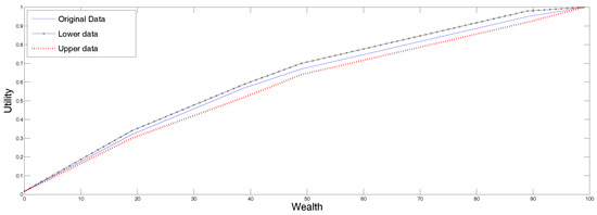
Figure 1.
Utility reconstruction from data in Table 1.
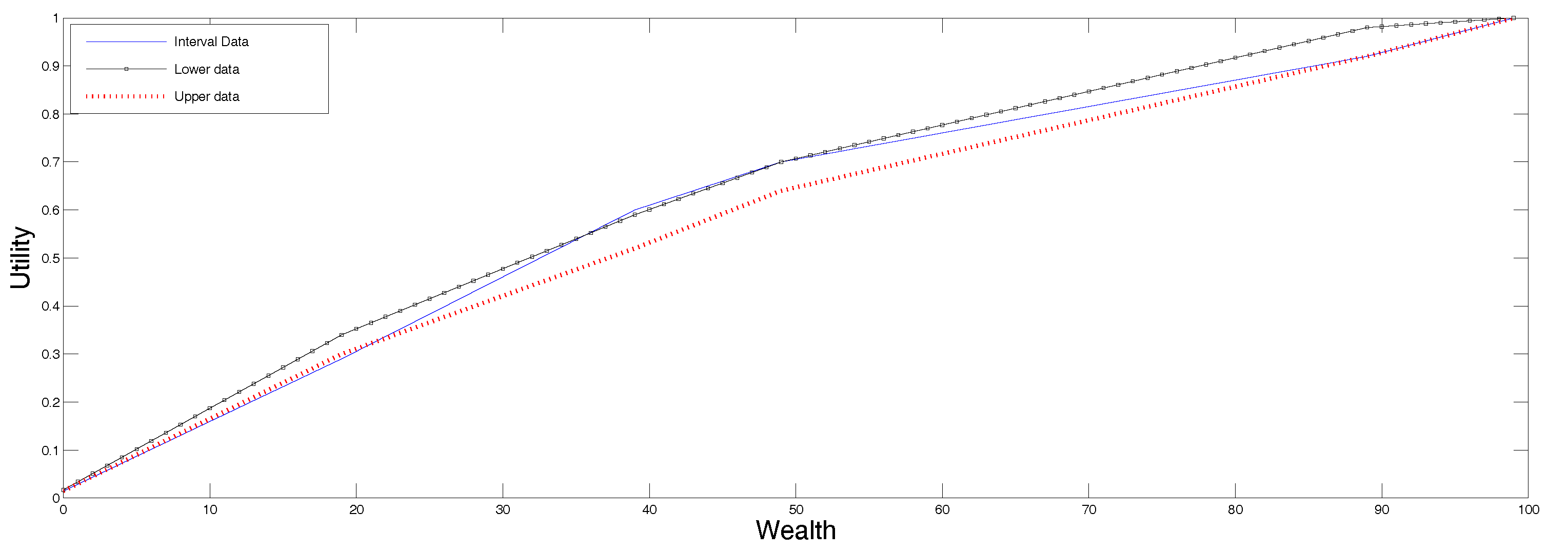
To continue with the example, in Figure 2 we present in continuous line, the reconstruction according to the SME procedure for data in ranges described in Section 4.2, and we plotted the two utility functions determined by the end points of the undecidability range for comparison. All these curves are in the same plot just to visualize them together, not for comparison purposes because they solve to different, albeit related problems. Note that now, the “true” utility falls within the range determined by the utilities corresponding to the upper and lower preference values.
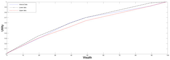
Figure 2.
Utility reconstructed from data in ranges in Table 1.
5.2. Luenberger’s Example with and without Uncertainty
This example is worked out in Luenberger [2] by means of a least squares minimization procedure applied to a power function that has the right convexity properties built in from the beginning. He chooses and recovers and which renders concave. The input data is presented in the original form in Table 2, and rescaled in Table 3.
Table 2.
Extended Luenberger’s example.
Table 3.
Standardized extended Luenberger’s table.
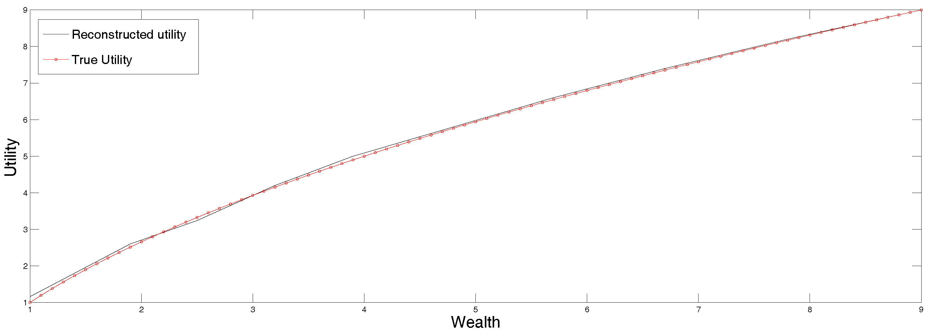
In Figure 3 we plot the original parametric curve (in dots), as well as the utility reconstructed by applying the standard maximum entropy method to the data in Table 3, the first row of which lists the certainty equivalents corresponding to the expected utilities listed in the second row. Clearly the agreement is quite good, and we did not have to guess the right parametric representation of the function.
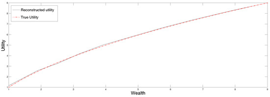
Figure 3.
Reconstructed utility from point data in Table 3.
In the third row of Table 2 and Table 3 we list some possible interval ranges of the utility function of an undecided decision maker (original and scaled down ranges). To show the usefulness of the maxentropic procedure when the data is given in ranges, we apply the maxentropic procedure for data in ranges explained in Section 4.2, to the data in the third row of Table 3, and display the utility function so obtained in Figure 4. Clearly, when the data is specified in ranges, it would be somewhat hard to apply a parametric fitting procedure. The maxentropic procedure produces an increasing and continuous function that stays within the specified utility range.
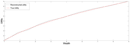
Figure 4.
Utility reconstructed from interval data of Table 3.
Now, to consider another variation on the theme, suppose that we want to make sure that the utility function has the right concavity (or convexity) properties. Certainly, a simple plot of the vales of the utility suggests that the utility must be concave. Thus, we might decide to consider the problem analyzed in Section 2, that is to reconstruct the second derivative of the utility function by means of the method of maximum entropy in the mean described in Section 4.3. Accordingly, we have to solve (9), where the vector m that is specified right below that equation to be used as input for the numerical analysis is given Table 4.
Table 4.
Modified Luenberger’s data.
Recall that the procedure of maximum entropy in the mean is used now to determine the second derivative of the utility function, from which the function itself is determined by simple integration.
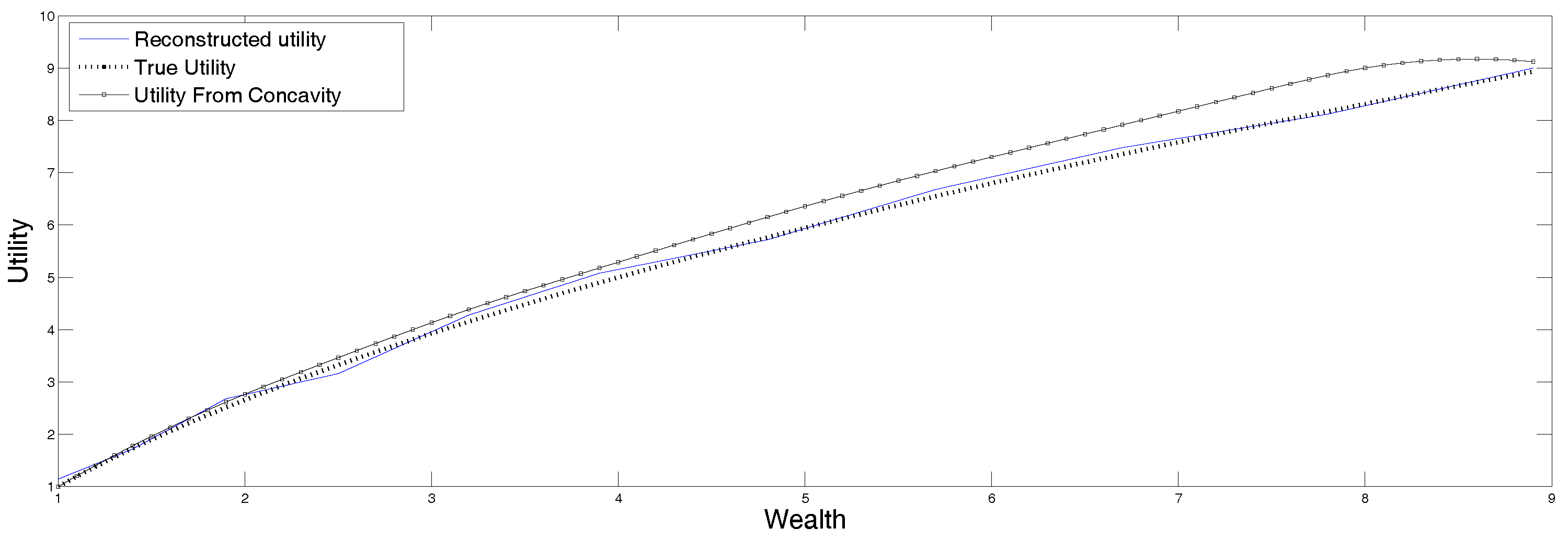
The reconstruction obtained from the data in Table 4 is displayed in Figure 5 along with the original function. Recall that the output of this procedure is the second derivative of the utility function, which is then integrated to recover the function itself. This reconstruction is very sensitive to the input data and the discretization procedure, that is why it is convenient to apply the version of MEM that allows for data in intervals as well as for errors in the data. The procedure was described in Section 4.5, and the result of applying it to the data listed in Table 5 is displayed in Figure 6 for two values of the parameter describing the size of the error.
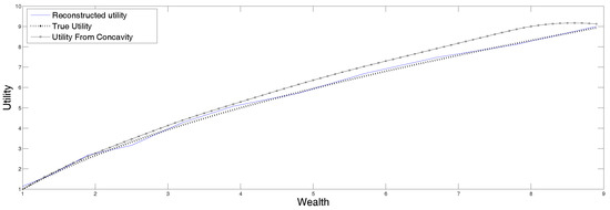
Figure 5.
Utility function from reconstructed second derivatives from data in Table 4.
Table 5.
Data for determining the function from reconstructed second derivative.
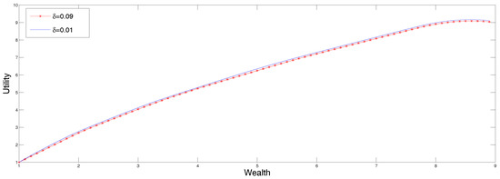
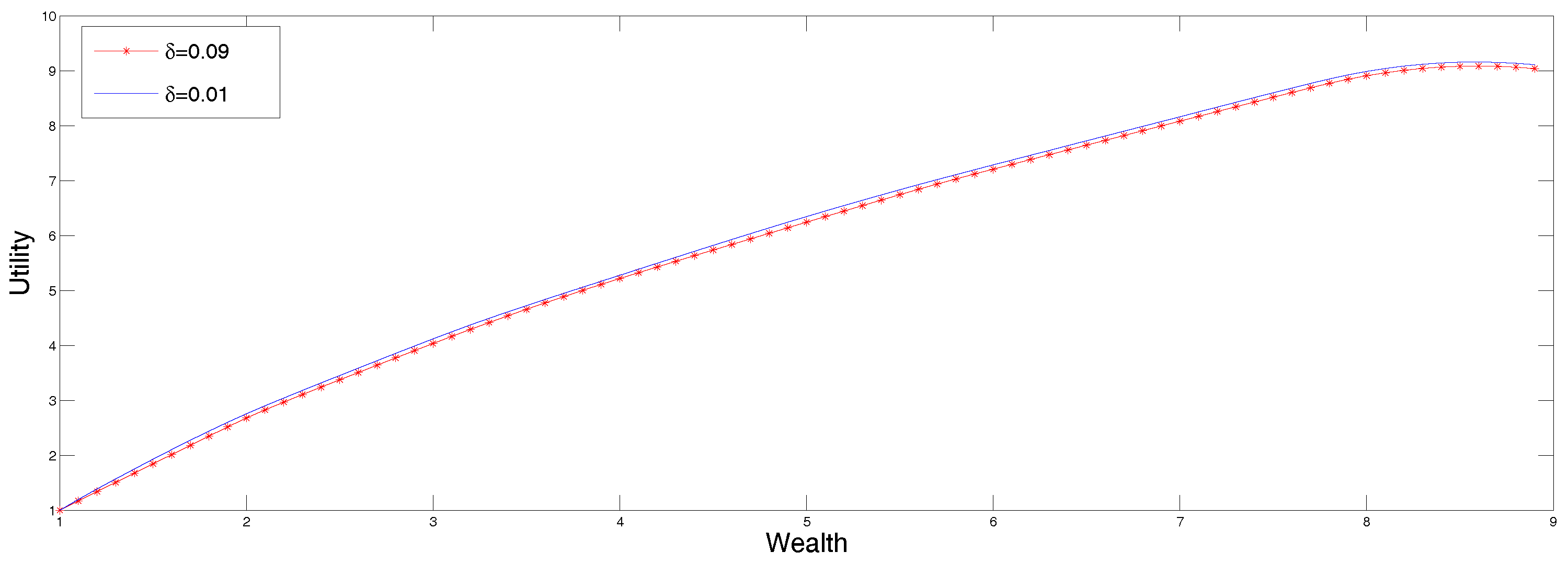
Figure 6.
Utility function from reconstructed second derivatives from data in Table 5.
The data in Table 5 corresponds to a decision maker that is slightly undecided. The two utility functions obtained from the reconstructed discretized second derivative according to the results presented in sections two and three. The displayed reconstructions correspond to and
In Figure 6 we present two utility functions obtained from the reconstructed discretized second derivative according to the results presented in Section 2 and Section 3. The displayed reconstructions correspond to and We mention that for values of the algorithm converges too slowly because the derivative of the dual entropy oscillates from one end of the reconstruction range to the other without converging to zero.
6. Concluding Remarks
To sum up and highlight the applications of utility theory, the problem of determining preferences from the expected value of a few random bets of from their certainty equivalents can be rephrased as an interpolation problem which can itself be transformed into a generalized moment problem. The moment problem can be extended to incorporate errors in the data and data in ranges. This would correspond to the case in which there are errors in the data of the utility function or that the utility is known up to a range. All of these problems can be solved by appropriate versions of the maximum entropy method.
Furthermore, when the risk preferences of the decision maker are known, the problem mentioned in the previous paragraph can be transformed into a problem consisting in solving a linear integral equation for a function with pre-specified signature. The method of the maximum entropy in the mean can be applied to solve that problem for us.
Acknowledgments
All sources of funding of the study should be disclosed. Please clearly indicate grants that you have received in support of your research work. Clearly state if you received funds for covering the costs to publish in open access.
Author Contributions
Both authors contributed equally to the paper. Both the authors have read and approed the final manuscript.
Conflicts of Interest
The authors declare no conflict of interest.
Abbreviations
The following abbreviations are used in this manuscript:
| SME | standard maximum entropy |
| MEM | maximum entropy in the mean |
| MDPI | Multidisciplinary Digital Publishing Institute |
| DOAJ | Directory of open access journals |
| TLA | Three letter acronym |
| LD | linear dichroism |
References
- Eeckhoudt, L.; Gollier, C.; Schlessinger, H. Economic and Financial Decisions under Risk; Princeton University Press: Princeton, NJ, USA, 2005. [Google Scholar]
- Luenberger, D. Investment Science; Oxford University Press: Oxford, UK, 1998. [Google Scholar]
- Herstein, I.; Milnor, J. An axiomatic approach to measurable utility. Econometrica 1953, 21, 291–297. [Google Scholar] [CrossRef]
- Abbas, A.E. An entropy approach for utility assignment in decision analysis. In Bayesian Inference and Maximum Entropy Methods in Science and Engineering; Williams, C.J., Ed.; Kluwer Academic: Dordrecht, The Netherlands, 2003; pp. 328–338. [Google Scholar]
- Abbas, A.E. Entropy methods for univariate distributions in decision analysis. In Bayesian Inference and Maximum Entropy Methods in Science and Engineering; Williams, C.J., Ed.; Kluwer Academic: Dordrecht, The Netherlands, 2003; pp. 329–349. [Google Scholar]
- Abbas, A. Maximum Entropy Distributions with Upper and Lower Bounds. In Bayesian Inference and Maximum Entropy Methods in Science and Engineering; Williams, C.J., Ed.; Kluwer Academic: Dordrecht, The Netherlands, 2005; pp. 25–42. [Google Scholar]
- Darooneh, A.H. Utility function from maximum entropy principle. Entropy 2006, 8, 18–24. [Google Scholar] [CrossRef]
- Dionisio, A.; Reis, A.H.; Coelho, L. Utility function estimation: The entropy approach. Phys. A 2008, 387, 3862–3867. [Google Scholar] [CrossRef]
- Pires, C.; Dionisio, A.; Coelho, L. Estimating utility functions using generalized maximum entropy. J. Appl. Stat. 2013, 40, 221–234. [Google Scholar] [CrossRef]
- Abbas, A.E. Maximum entropy utility. Oper. Res. 2006, 54, 277–290. [Google Scholar] [CrossRef]
- Mettke, H. Convex cubic Hermite-spline interpolation. J. Comp. Appl. Math. 1983, 9, 205–211. [Google Scholar] [CrossRef]
- Lai, M.J. Convex preserving scattered data interpolation using bivariate cubic splines. J. Comp. Appl. Math. 2000, 119, 249–258. [Google Scholar] [CrossRef]
- Visnawatahan, P.; Chand, A.K.B.; Agarwal, R.P. Preserving convexity through rational cubic spline fractal interpolation. J. Comp. Appl. Math. 2014, 263, 262–276. [Google Scholar] [CrossRef]
- Dybvig, P.H.; Rogers, L.C.G. Recovery of preferences from observed wealth in a single realization. Rev. Fin. Stud. 1997, 10, 151–174. [Google Scholar] [CrossRef]
- Cox, A.M.G.; Hobson, D.; Obłój, J. Utility theory front to back–inferring utility from agents choice’s. Int. J. Theor. Appl. Financ. 2014, 17, 1450018:1–1450018:14. [Google Scholar] [CrossRef]
- Buchen, P.W.; Kelly, M. The maximum entropy distribution of an asset inferred from option prices. J. Finan. Quant. Anal. 1996, 31, 143–159. [Google Scholar] [CrossRef]
- Stutzer, M. A simple non-parametric approach to derivative security valuation. J. Fin. 1996, 51, 1633–1652. [Google Scholar] [CrossRef]
- Gulko, L. The entropy theory of bond option pricing. Int. J. Theor. Appl. Fin. 1999, 5, 355–383. [Google Scholar] [CrossRef]
- Zhou, R.; Cai, R.; Tong, G. Applications of entropy in finance: A review. Entropy 2013, 15, 4909–4931. [Google Scholar] [CrossRef]
- Jaynes, E.T. Information theory and statistical mechanics. Phys. Rev. 1957, 106, 620–630. [Google Scholar] [CrossRef]
- Gomes-Gonçalvez, E.; Gzyl, H.; Mayoral, S. Density reconstructions with errors in the data. Entropy 2014, 16, 3257–3272. [Google Scholar] [CrossRef]
- Navaza, J. The use of non-local constraints in maximum entropy electron density reconstruction. Acta Crystallog. 1986, 42, 212–233. [Google Scholar] [CrossRef]
- Dacunha-Castelle, D.; Gamboa, F. Maximum d’entropie et probleme des moments. Ann. Inst. Henri Poincaré 1990, 26, 567–596. (In French) [Google Scholar]
- Golan, A.; Judge, G.G.; Miller, D. Maximum Entropy Econometrics: Robust Estimation with Limited Data; Wiley: New York, NY, USA, 1996. [Google Scholar]
- Golan, A.; Gzyl, H. A generalized maxentropic inversion procedure for noisy data. Appl. Math. Comp. 2002, 127, 249–260. [Google Scholar] [CrossRef]
- Gzyl, H.; Velásquez, Y. Linear Inverse Problems: The Maximum Entropy Connection; World Scientific Publishers: Singapore, 2011. [Google Scholar]
- Gzyl, H.; Mayoral, S. Determination of risk measures from market prices of risk. Insur. Math. Econom. 2008, 43, 437–443. [Google Scholar] [CrossRef]
- Gzyl, H.; Mayoral, S. A method for determining risk aversion from uncertain market prices of risk. Insur. Math. Econom. 2010, 47, 84–89. [Google Scholar] [CrossRef]
- Gzyl, H.; ter Horst, E. A relationship between the ordinary maximum entropy method and the method of maximum entropy in the mean. Entropy 2014, 16, 1123–1133. [Google Scholar] [CrossRef]
- Borwein, J.; Lewis, A. Convex Analysis and Non-Linear Optimization; CMS Books in Mathematics; Springer: New York, NY, USA, 2000. [Google Scholar]

© 2017 by the authors. Licensee MDPI, Basel, Switzerland. This article is an open access article distributed under the terms and conditions of the Creative Commons Attribution (CC BY) license (http://creativecommons.org/licenses/by/4.0/).