Abstract
Terms related to gradients of scalar fields are introduced as scalar products into the formulation of entropy. A Lagrange density is then formulated by adding constraints based on known conservation laws. Applying the Lagrange formalism to the resulting Lagrange density leads to the Poisson equation of gravitation and also includes terms which are related to the curvature of space. The formalism further leads to terms possibly explaining nonlinear extensions known from modified Newtonian dynamics approaches. The article concludes with a short discussion of the presented methodology and provides an outlook on other phenomena which might be dealt with using this new approach.
1. Introduction
Recent work on entropic gravity by Erik Verlinde [1,2] has initiated a recovery of earlier work by the author on the thermodynamics of diffuse interfaces [3] and stimulated a generalization of this approach. The approach depicted in the present article draws on a combination of the very forceful and fundamental concepts of entropy, of the phase-field method and of the Lagrange formalism. The capability of this approach to describe various aspects of gravity will ultimately be demonstrated.
The description of entropy has up to now been based on the use of scalars for the probabilities of the individual states :
The scope of the present article is to generalize the entropy formulation and to include terms related to vectors (with options for future extension to tensors) within a formulation:
Known conservation laws for energy E, mass M, charge Q, momentum , and spin , where each law is formulated as a function of are then added as constraints to the variational problem. Each constraint is associated with its own Lagrange multiplier (λ, g, ε,…) yielding, in total, a free energy density f:
The Lagrange multipliers and for momentum and spin , respectively, obviously have to be vectors in order to recover a scalar contribution to the overall scalar equation. Units and scales are implicitly introduced through the Lagrange multipliers. The Lagrange multiplier λ, for example, corresponds to = making the energy dimensionless (or, giving the dimension of kT to entropy/probability). The names of the Lagrange multipliers have been arbitrarily selected to be similar to the names of known fundamental constants, and have been assigned to the conservation law to which they are most probably related. Relations between these constants are expected to emerge from the Lagrange formalism being applied to above free energy density.
The Lagrange formalism is based on a free energy functional F being the volume integral of a free energy density f. Its variational derivative corresponds to:
Executing these derivatives provides the equations of motion of the system. The present paper will demonstrate the initial results obtained when applying the above scheme to mass conservation. However, the paper will not address any time-dependent phenomena, that is, no dependencies on will be considered in the Lagrange density.
2. Entropy
The proposed concept requires a formulation of entropy which comprises terms related to vectors (and in future also time derivatives). In order to specify vectors, a reference frame and/or a coordinate system has to be defined. In spite of introducing vectors (or tensors) into the terms of the equations, the overall entropy formulation and all the probabilities entering into the typical logarithmic terms have to remain scalars.
2.1. Scalar Entropy
Entropy has revealed its importance in numerous fields. Some of the most important discoveries are based on entropy such as, for instance, (i) the Boltzmann factor in energy levels of systems; (ii) the Gibbs energies of thermodynamic phases; (iii) the Shannon entropy in information systems; (iv) the Hawking entropy of black holes; (v) the Flory-Huggins polymerization entropy in polymers [4,5]; and (vi) the crystallization entropy in metals [4,6], to name only some of the major contributions.
All of these approaches for entropy are typically based on logarithmic terms such as (see e.g., [7]):
It seems important to note that entropy can be interpreted as tending to smear out any contrast between different states and/or different objects. The contrast between states/objects is reflected in gradients of an observable property allowing one to distinguish between these states/objects. Any object can be defined as a coherent region of space, which can be distinguished from other regions due to a contrast in at least one attribute/property. This attribute may even be the “name” of the object indicating that one—based on some criterion—has identified the region as belonging to the same object [8].
Gradients and interfaces, i.e., measures of contrast, are thus most important for describing physical objects and should be reflected in the formulation of the entropy. For example, a sphere is an object having the maximum entropy for a given volume. The next section thus describes an approach for introducing gradients into the entropy formulation, i.e., making the step from the “scalar” entropy based on scalar values , to the “gradient” entropy also comprising gradients .
2.2. Entropy Formulations Comprising Gradient Terms
The name “gradient entropy” is misleading because the value of the entropy, and also the probabilities entering into its formulation, remain scalars even if gradients are present in its formulation. The choice of another name might thus be meaningful in future. The “gradient entropy” described in a previous work [3] aimed at describing the growth of crystals using a phase-field approach (see Section 3). Its relevant content is briefly summarized in the following.
Classical thermodynamics is based on Gibbs formulation of the following variational problem [7]:
where are the Lagrange multipliers accounting for the constraints of energy and probability conservation. The solution of this variational problem yields the well-known relation for the probability of a specific state :
where Z is the partition function which is necessary to normalize the probabilities, and . It is interesting to note that, instead of the simple variation the full variational derivative also leads to the same result since there are no explicit dependencies on gradients in the—equivalent—formulation:
Replacing the logarithmic terms by scalar products of type drastically changes that situation. Under some simplifying assumptions—especially a Taylor expansion of the logarithmic terms—scalar products comprising gradients occur [3]:
The presence of such gradient terms has major consequences for the variational procedure as the operator now finds a target. To physically motivate this replacement of the logarithmic terms by scalar products, it is helpful to consider models of crystal growth as depicted below.
Interfaces in physical systems often have a finite extension of several monolayers and it, therefore, seems meaningful that the extension of thermodynamics, which includes sharp interfaces, to a more general thermodynamic description involves diffuse interfaces and/or gradients. Two discrete models describing the growth of a so called Kossel crystal, Figure 1a, will be described in more detail: (i) the Jackson model of faceted growth [6], Figure 1b; and (ii) the Temkin model for the growth of a diffuse interface [9], Figure 1c.
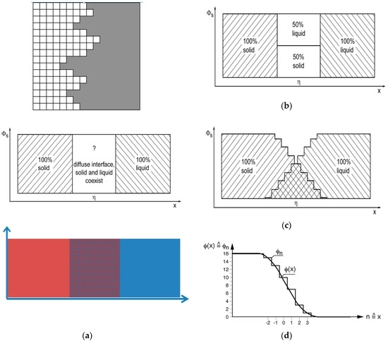
Figure 1.
(a) Kossel’s model of a growing crystal (figure adapted from [4]). Atoms attach to the interface in layers. The model assumes that the atoms may only adhere to the top of already solid atoms (‘solid on solid’). A smooth transition with a finite interface thickness can be identified when averaging the fraction of solid atoms parallel to the interface (see Figure 1d). (b) The Jackson model [6] assumes an interface which is restricted to a single layer separating the two bulk regions. The entropic term in the Jackson model reads: ΦlnΦ + (1−Φ)ln(1−Φ). (c) The Temkin model [9] assumes multiple steps separating the two bulk regions. The entropy of an intermediate layer n in this case is also defined by its adjacent layer n − 1. The entropic term in the Temkin model reduces to the Jackson model in the case of a single interface layer and reads: (* see footnote of Equation (10)). (d) The Schmitz model [3] is an extension of the Temkin model for small step widths and approximates the discrete formulation of Temkin by a continuous gradient and by turning the sum of the individual contributions of the discrete layers into an integral (see text): .
The Schmitz model [3], Figure 1d, extrapolates the discrete approach of Temkin into a continuum description, where the gradient may be identified by:
where, “” denotes the lattice spacing in the z-dimension. In contrast to the rest of the document the ∆*) in this equation and also in Figure 1c denotes a difference and not the Laplacian operator. Generalization to three dimensions then yields where represents a vector characterizing the metric imposed by the underlying crystal structure of the solid phase. The inclusion of such gradient type contributions due to diffuse interfaces—revealing a characteristic length scale defined by the vector —in the classical free energy/entropy formulation of thermodynamics is extremely interesting for the description of evolving structures, and introduces a length scale into thermodynamics.
In the case of multiple objects “i”, each of these objects will have its own order parameter , and its own interface which is characterized by as depicted in Section 3 on phase field models. Variational minimization of the resulting free energy functional for N objects comprising entropic terms of type:
recovers the phase-field equations of motion under specific, simplifying assumptions. One of these assumptions relates to a Taylor expansion of the terms which, for provides the following approximation:
The scalar character of the entropy has been maintained by using scalar products when inserting the gradient terms. The vector in this early model [3] corresponds to the lattice vector of the growing crystal which determines the distance between individual, discrete atomic layers of the Temkin model.
No such vector is a priori specified for a more generic formulation which is the objective of the present work. Thus, there is a need to specify a reference vector which plays the role of the crystal lattice vector in the early crystallization model [3]. This vector has to be introduced as part of a scalar entity and the use of a scalar product, thus, seems mandatory. An interesting option for the choice of is the use of the scalar-triple (or parallelepipedal) product, Figure 2, spanning a volume having a value v together with an oriented coordinate system consisting of the three base vectors :
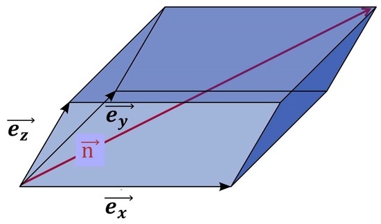
Figure 2.
Scalar triple product: The volume being spanned by these vectors is v. The diagonal vector of this coordinate system reads with its norm being in the case of an orthonormal system. This vector is also the normal vector to the tangential plane to that volume.
A periodic repetition of this elementary finite volume may ultimately fill the entire space and can be approximated by a continuous field . For the purpose of this paper, the norm of the vector and the volume of the parallelepiped v are considered as constants.
Terms including scalar products between the coordinate system defined by and gradients of the scalar fields then—in analogy with Equation (12)—read:
3. Phase-Field Models
The overall strategy of the methodology proposed in this article comprises compiling the free energy density from a combination of entropic terms (see previous section) and constraints given by conservation laws. The specification of multiple becomes mandatory for describing different objects and also for formulating the constraints of mass, energy and momentum conservation in terms of the variables :
The basis for dealing with this task is provided by the phase-field method which will be briefly reviewed in terms of its relevance for the scope of the present methodology.
Phase-field models have their origin in the description of phase transitions. Phase transitions play a vital role in many areas of physics at all scales including, for instance, magnetism, superconductivity, solidification, condensation, solid state transformations, very fundamental transitions like the Higgs-Kibble mechanism unifying electroweak interaction and, possibly, even the nucleation and growth of galaxies.
Theories of phase transitions have their origin in the early models of van der Waals (1893), Korteweg (1901), Ginzburg-Landau (1950), Cahn-Hilliard (1958), Allen-Cahn (1960), Halperin, Hohenberg and Ma (1977). While the early models did not include any spatial resolution, especially the Cahn-Hilliard equation which, for the first time, addressed demixing phenomena using a spatially-resolved approach. The order parameter entering into the equations was the—conserved—concentration of alloy elements. The Allen-Cahn equation then included the option of non-conserved order parameters for the first time. It seems essential to highlight that phase transitions are best described by non-conserved order parameters such as, for example, the fraction liquid of a system will change from 1 to 0 in a solidification process and is thus not a conserved quantity.
The first phase-field concept was proposed in an unpublished work by Langer [10] and was first publicly documented by Fix [11] and Caginalp [12]. The simulation of the evolution of complex 3D dendritic structures using phase-field models by Kobayashi [13] initiated extensive use of this methodology in materials sciences. The binary transitions/equilibria between two states were later extended to multi-phase equilibria in a multi-phase-field-model [14]. Higher order derivatives of the order parameter eventually lead to atomic resolution of rigid lattices in so called phase-field crystal models [15]. Currently, phase-field models have reached a high degree of maturity and found applications in describing complex microstructures in technical alloy systems [16]. Reviews on phase-field modelling are found, for instance, in [17,18].
The core of most phase-field models is the description of the evolution of the shape of an object in time. To describe the evolution of this shape it is necessary, as a first step, to mathematically describe the initial shape of the object, Figure 3:
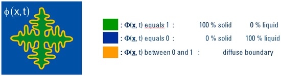
Figure 3.
Basic setting for the description of a complex shaped object by an order parameter. The order parameter field takes the value 1 wherever and whenever the object is present. A diffuse continuous interface marks the transition from the object to the “non-object”, as shown here for a solid object in a liquid.
This initial shape is, thus, expressed as a scalar field of an “order parameter”, which is alternatively named “feature indicator” or, most commonly, a “phase–field variable”. For the present objective, it is sufficient to restrict further discussion to rigid objects. Neither the evolution of their shape nor their motion in vacuum space will be addressed here. The most basic use of a phase-field model is to just draw on the definition of the “phase-field”-variable. The phase field description of a static object—here a sphere—placed in a vacuum is schematically depicted in Figure 4.
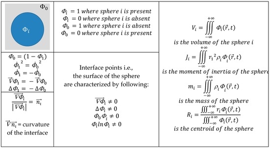
Figure 4.
Some important mathematical relations related to the phase-field description of a massive sphere.
The mass of a sphere i then is given as:
It should be noted that the integral extends over the entire space and not only covers the domain of the sphere. Here, the phase-field variable —which is 0 outside the sphere i–acts as a type of stencil selecting the domain of the sphere from infinite space. The conservation for a total mass of a system of N objects/spheres is then given by:
where the index I = 0 refers to the vacuum. Specifying the total mass as the integral of an average mass density:
allows one to formulate the constraint for mass conservation as follows:
If only a maximum of two objects coexist at the same point, e.g., at the interface between vacuum and a massive object with index i, it is possible to rewrite the function as yielding:
This assumption holds everywhere and at all times, as long as the massive objects are immersed in a vacuum and do not have any mutual contact. The mass density of the vacuum will become important in view of the cosmological constant entering into the scheme in this way (see Section 5).
4. Lagrange Formalism
Similar to entropy, the Lagrange formalism also plays a significant role in many areas of physics. In addition to the derivation of the Boltzmann factor depicted above, the Lagrange formalism is a major foundation for quantum mechanics and, in particular, has been used to derive relations between symmetries and conservation laws. The Noether theorems, which were derived using the Lagrange formalism, showed that invariance of physical laws subject to a translation implies the conservation of momentum and invariance subject to translation in time implies the conservation of energy. A further striking observation is that major physical laws all contain a Laplacian operator (that is, are a Poisson-type equation) somehow suggesting a common ground of all these models, which comprise all different length scales like gravitation, electrostatics, thermal conductivity, diffusion, flow, phase-field, Schrödinger equations, density functional equations and many others. Some operators present in the Lagrange scheme have the property of generating Laplacian operators.
The basic concept of the Lagrange formalism is based on a functional being a scalar function F of a variable which, itself, is a function of space and time and being an integral of a density function f.
The density function f is a function of a number of variables especially comprising :
The fundamental Lagrange formalism allows for extensions to further variables, to higher order derivatives and also to tensor fields. The present article will only consider first order derivatives. Setting the variation of F to zero with respect to one of the variables provides the corresponding Euler equation by setting the variational derivative of the function f to zero:
The results are the desired equations of motion for the different .
5. Derivation of the Gravitational Law
The entropy for the static field as formulated in Chapter 2 in Taylor approximation reads:
The scalar product for the square term here has been formally executed introducing a cos2 function of the angle between the vectors . When applying the Lagrange formalism, this cos2 function will eventually lead to a non-linear generalization of the Newton–Poisson equation as, for instance, that used in the modified Newtonian dynamic (MOND) approaches [19,20,21,22]. Further aspects of this generalization are detailed and discussed in Section 6. In the following, the function is first considered as a constant making the product . The overall entropy term only comprises terms related to and no terms related to . Thus, only the gradient related terms of the functional derivative become active in the Lagrange formalism:
Executing this derivative yields:
The Poisson equation can be immediately identified. The divergence of the normal vector of a surface is the measure of the curvature of that surface. The vector is the diagonal of the volume and perpendicular to the tangential plane to that volume. The divergence of this vector is, thus, a measure for the curvature κ of space.
The constraint for mass conservation—its specification being fully detailed in Equations (18) and (19)—is associated with the Lagrange multiplier g and only depends on . This constraint does not contain any terms related to :
Overall, the following equation for the field arises when adding this constraint term (26) to the term for the entropy Equation (25):
Using the special formulation for the constraint of mass conservation comprising also the density of the vacuum (Equation (19)), generates an additional term:
Calibrating the Lagrange multiplier g to 8πG with G being the gravitational constant yields:
By comparing with the cosmological constant Λ [23]:
allows one to rewrite Equation (29) as:
By neglecting the curvature κ of space (i.e., setting and setting this equation becomes identical with the Poisson equation of gravitation, i.e., with classical Newton’s law:
To summarize this, the application of the Lagrange scheme to the gradient-entropy terms as depicted in the present paper obeying the constraint of mass conservation has led to a strikingly direct derivation of:
- the Poisson equation of gravity (Newton’s law);
- a term related to curvature of space (which can probably be related to Einstein’s general theory of relativity);
- a term introducing the mass density of vacuum (which seems related to the cosmological constant); and
- terms related to a nonlinear generalization of the Newton–Poisson equation as used in modified Newtonian dynamic (MOND) approaches [19,20,21,22].
These MOND terms will be discussed in more detail in the following section.
6. Modified Newtonian Dynamics
Formulations and equations in Modified Newtonian Dynamics (MOND) approaches [19,20,21,22] are constructed based on experimental findings and are fitted to the experimental observations: especially to velocity distributions in galaxies. These approaches do not draw on dark matter as the basis for describing the observed behavior. In spite of successfully describing the experimental observations, the MOND formulations are involved in controversial discussions since they still lack a deeper theoretical framework for their derivation from fundamental principles. The present work indicates a possible approach towards a deeper understanding of the background of the empirical MOND equations.
This chapter aims to elucidate relations of the proposed approach to the modified Newtonian dynamics (MOND) already briefly indicated in Section 2. Recovering the equation for the gradient entropy from Chapter 2, also including the curvature related term, reads:
where the angle between the space diagonal and the gradient of the scalar field is denoted as . The variational derivative then looks as follows:
which, with:
leads to:
For small angles of , sin() ~ 0 and tan2(φ) ~ 0, the classical Newton-Poisson equation is recovered, while for angles of φ approaching , the MOND terms generate additional contributions. In both cases, the curvature related term persists. For comparison, the MOND Eulerian [20] reads:
where μ(x) is “….an as-yet unspecified function (known as the “interpolating function”), and a0 is a new fundamental constant (a0~10−8 cm s−2) which marks the transition between the Newtonian and deep-MOND regimes. Agreement with Newtonian mechanics requires μ(x) → 1 for x >> 1, and consistency with astronomical observations requires μ(x) → x for x << 1. Beyond these limits, the interpolating function is not specified by the theory, although it is possible to weakly constrain it empirically……” [20]. Examples for the MOND interpolation function are the “standard” [22] and the “simple” [24] interpolation functions:
On setting the term corresponds to the square of the “standard” interpolation function. Setting directly yields the “simple” interpolation function.
In spite of these similarities with the MOND type formulations, there are also obvious differences, such as (i) the persistence of the original Newton term; (ii) the negative sign of the MOND_I term; (iii) the new, additional term denoted as MOND_II; (iv) the term likely to be related to “Einstein” curvature, and (v) the “Λ term”, see Equation (31).
It seems most interesting to ultimately elaborate a relation and a physical interpretation for the angle φ between the gradient of the potential and the direction of the diagonal vector of the underlying coordinate system. A possible geometric interpretation in two dimensions is depicted in Figure 5:
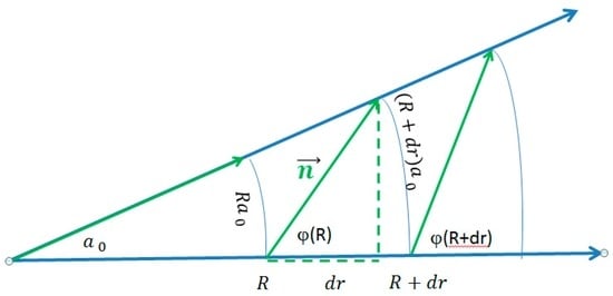
Figure 5.
The proposed explanation for a change in the direction of the normal vector of space leading to an angle φ which increases with increasing radius R (see text).
The area A(R) of a small segment between R and R + dr being bounded by the angle α0 reads:
Postulating that this area A of the parallelepiped having the diagonal to be constant when increasing the radius R by dr requires:
where is a proportionality constant having dimensions (L2). The tangent of the angle between the radial direction and the diagonal of the parallelepiped, can then be approximated as a function of R by:
where is a yet undefined constant probably related to the parameter in the MOND approaches, which indicates the transition between Newtonian and MOND regimes. In spite of being most interesting, it is beyond the scope of the present article to further elucidate the origin and interpretation of this angle and/or the value of .
In summary, it was possible to obtain the following equation for gravity when formally performing, to its full extent, the proposed scheme:
This equation comprises a combination of terms similar—at least in a qualitative way—to those appearing in a number of other theories of gravitation. In its simplest approximation, i.e., for:
this equation—derived from a mere entropic approach—clearly recovers the classical Newtonian law. All other terms remain subject to future discussions.
7. Summary and Future Perspectives
The approach for the description of gravity modeled in the present article is based on: (i) an entropy formulation comprising scalar products of gradients of a scalar field with (ii) the diagonal vector of a volume element; (iii) a field description of objects being based on this scalar field; and (iv) a formulation of the constraint for mass conservation in terms of this scalar field. Performing (v) the Lagrange formalism onto the resulting formulations in a strikingly direct derivation has led to:
- the Poisson equation of gravity (Newton’s law);
- a term related to the curvature of space (which probably can be related to Einstein’s general theory of relativity);
- a term introducing the mass density of vacuum (which seems related to the cosmological constant);
- terms related to a nonlinear generalization of the Newton–Poisson equation as used in modified Newtonian dynamic (MOND) approaches.
The resulting formulation suggests a co-existence with respect to a superposition of different types of models being currently intensely discussed. A deeper investigation and interpretation of the presented approach by the respective communities thus seems worth some effort. It should be noted that the present paper has only touched on a subset of an overall scheme, which may be extended in several directions as depicted in Table 1.

Table 1.
Basic scheme to derive equations of motion using a Lagrange formalism acting on different entropy formulations being constrained by different conservation laws.
The mass constraint, in particular, investigated in the present article can, and should, be replaced by the energy-momentum tensor in a relativistic formulation. A number of further, open questions remain to be addressed, such as (i) the origin and interpretation of the angle ϕ in the formulations, (ii) the origin and interpretation of the length scale (L2) introduced by the scalar products, (iii) a careful comparison with other theories, and (iv) a comparison with experimental observations.
The appealing simplicity of the approach provides an interesting, new and alternative view on things and perhaps provides an even a better understanding of phenomena in the future. This appears to make the approach deserving of further research.
Acknowledgments
The ideas being documented in the present article have emerged over several years in parallel to ongoing projects being funded by various institutions. However, the efforts toward compiling these ideas did not receive any dedicated funding. Covering the costs for open source publication by my employer ACCESS e.V. is gratefully acknowledged. Thanks are due to the MICRESS® group at ACCESS e.V. for numerous discussions and constructive criticism. Special thanks are due to Bernd Böttger, Gottfried Laschet, and Markus Apel for commenting on the final manuscript and to Ulrike Hecht for drawing my attention to the MOND at just the right time.
Conflicts of Interest
The author declares no conflict of interest. The founding sponsors had no role in the design of the study; in the collection, analyses, or interpretation of data; in the writing of the manuscript, and in the decision to publish the results.
References
- Verlinde, E.P. On the Origin of Gravity and the Laws of Newton. J. High Energy Phys. 2011, 29. [Google Scholar] [CrossRef]
- Verlinde, E.P. Emergent Gravity and the Dark Universe. arXiv 2016. [Google Scholar]
- Schmitz, G.J. Thermodynamics of diffuse interfaces. In Interface and Transport Dynamics; Emmerich, H., Nestler, B., Schreckenberg, M., Eds.; Springer Lecture Notes in Computational Science and Engineering; Springer: Berlin/Heidelberg, Germany, 2003; pp. 47–64. [Google Scholar]
- Woodruff, D. The Solid Liquid Interface; Cambridge University Press: Cambridge, UK, 1973. [Google Scholar]
- Flory, P.J. Principles of Polymer Chemistry; Cornell University Press: New York, NY, USA, 1953. [Google Scholar]
- Jackson, K.A. Liquid Metals and Solidification; ASM: Cleveland, OH, USA, 1958. [Google Scholar]
- Jaynes, E.T. Probability Theory: The Logic of Science, Chapter 11. Available online: http://omega.albany.edu:8008/JaynesBook.html) (accessed on 30 March 2017).
- Schmitz, G.J.; Böttger, B.; Apel, M.; Eiken, J.; Laschet, G.; Altenfeld, R.; Berger, R.; Boussinot, G.; Viardin, A. Towards a metadata scheme for the description of materials—The description of microstructures. Sci. Technol. Adv. Mater. 2016, 17, 410–430. [Google Scholar] [CrossRef] [PubMed]
- Temkin, D.E. Crystallization Processes; Sirota, N.N., Gorskii, F.K., Varikash, V.M., Eds.; English Translation; Consultants Bureau: New York, NY, USA, 1966. [Google Scholar]
- Langer, J. Manuscript on a concept of phase field models. 1978; unpublished work. [Google Scholar]
- Fix, G. Phase field models for free boundary problems. In Free Boundary Problems Vol. II; Fasano, A., Primicerio, M., Eds.; Piman: Boston, MA, USA, 1983. [Google Scholar]
- Caginalp, G.; Fife, P.C. Phase-field methods for interfacial boundaries. Phys. Rev. B 1986, 33, 7792–7794. [Google Scholar] [CrossRef]
- Kobayashi, R. Modeling and numerical simulations of dendritic crystal growth. Physica D 1993, 63, 410–423. [Google Scholar] [CrossRef]
- Steinbach, I.; Pezzolla, F.; Nestler, B.; Seeßelberg, M.; Prieler, R.; Schmitz, G.J.; Rezende, J.L.L. A phase field concept for multiphase systems. Physica D 1996, 94, 135–147. [Google Scholar] [CrossRef]
- Elder, K.R.; Katakowski, M.; Haataja, M.; Grant, M. Modeling Elasticity in Crystal Growth. Phys. Rev. Lett. 2002, 88, 245701. [Google Scholar] [CrossRef] [PubMed]
- Schmitz, G.J.; Böttger, B.; Eiken, J.; Apel, M.; Viardin, A.; Carré, A.; Laschet, G. Phase-field based simulation of microstructure evolution in technical alloy grades. Int. J. Adv. Eng. Sci. Appl. Math. 2010, 2, 126–129. [Google Scholar] [CrossRef]
- Provatas, N.; Elder, K. Phase-Field Methods in Materials Science and Engineering; Wiley VCH: Weinheim, Germany, 2010. [Google Scholar]
- Steinbach, I. Phase-field models in Materials Science–Topical Review: Modelling Simul. Mater. Sci. Eng. 2009, 17, 073001. [Google Scholar]
- Bekenstein, J.; Milgrom, M. Does the missing mass problem signal the breakdown of Newtonian gravity? Astrophys. J. 1984, 286, 7–14. [Google Scholar] [CrossRef]
- Modified Newtonian Dynamics. Available online: https://en.wikipedia.org/wiki/Modified_Newtonian_dynamics (accessed on 30 March 2017).
- Milgrom, M. The MOND. Available online: https://arxiv.org/pdf/1404.7661.pdf (accessed on 30 March 2017).
- Milgrom, M. A modification of the Newtonian dynamics as a possible alternative to the hidden mass hypothesis. Astrophys. J. 1983, 270, 365–370. [Google Scholar] [CrossRef]
- Die kosmologische Konstante. Available online: https://de.wikipedia.org/wiki/Kosmologische_Konstante (accessed on 30 March 2017).
- Famaey, B.; Binney, J. Modified Newtonian Dynamics in the Milky Way. Mon. Not. R. Astron. Soc. 2005, 363, 603–608. [Google Scholar] [CrossRef]
© 2017 by the author. Licensee MDPI, Basel, Switzerland. This article is an open access article distributed under the terms and conditions of the Creative Commons Attribution (CC BY) license (http://creativecommons.org/licenses/by/4.0/).