Complexity and Vulnerability Analysis of the C. Elegans Gap Junction Connectome

1. Introduction

It is increasingly clear that the specific connectivities of biological networks are far from random. In neuroscience, the overall behavior and dynamics of a neuronal network is dictated both by the properties of individual neurons, and by the specific complex structure of the network through which they are connected [1,2]. Understanding the behavior of such a neuronal network must therefore involve inferring its underlying structural properties and design principles. However, it is unclear a priori which structural features of a network are most important in doing so. Distinguishing these important features is one of the goals in quantifying the complexity of a network, as a measure of network complexity could allow us to determine which features of a network cause it to be complex, and to infer then the purpose of these complex structures.

As of yet, there exists no broadly accepted definition of network complexity which would allow for its unambiguous quantification, though many quantitative measures have been proposed and applied [3,4]. A necessary property of any such measure, however, is that it must distinguish complex, structured networks from networks which are either completely random or completely ordered. One such measure was developed by Sakhanenko and Galas [5] who defined a general complexity measure, based in the Kolmogorov complexity, which correctly vanishes in these limiting cases. Indeed, even this simple approach appears capable of indicating certain complex structures existing within the network [5,6].

If a network is determined via some measure to be highly complex, the question yet remains: what is the source of that complexity? That is, what are the substructures or features of the network which make it “complex”? Can these measures be applied in such a way so as to identify complexity-causing structures within the network, and can we attribute biophysiological meaning to these structures?

The nematode C. elegans is an ideal system in which to attempt to address such questions. It remains the only organism for which the full connectivity of its neuronal network (its “Connectome”) is known. The C. elegans Connectome consists of both directed synaptic connections and undirected gap junction connections among its 302 neurons [7]. These neurons can be broadly classified as sensory neurons (those receiving external sensory input), motorneurons (those synapsing onto muscle), or, otherwise, as interneurons (if lacking explicit sensory input or motor output) [7]. Despite not directly receiving external input or driving motor output, many interneurons play important computational roles in the network. For example, the “command” interneurons are individually crucial to the control of locomotion; for example, if the command interneuron pair AVAL/R is ablated, the ability of the worm to crawl backwards is severely diminished, whereas ablating the command interneuron pair AVBL/R diminishes the ability of the worm to crawl forwards [8].

Even with its relatively small nervous system, C. elegans is capable of a fairly broad range of behaviors. In addition to responding to a range of mechanical and chemical stimuli [8,9,10], the worm must navigate [11], mate [12,13], and lay eggs [14,15]. The network controls these various behaviors through shared pathways of overlapping subcircuits, all while the structure appears to approximately minimize the wiring cost between nodes [16]. Previous studies indicate that, as with other neuronal networks [17,18,19,20,21,22,23], the network partially accomplishes this trade-off through its “rich club” structure, having a highly-connected hub of “rich” neurons with high betweenness centrality [24]. The specifically-tuned complex structure of the network may ultimately encode behavioral responses to inputs. For example, simulations of Connectome dynamics which treat all neurons as identical units are capable, through their connectivity structure alone, of generating biophysiologically reasonable dynamical responses to specific inputs (e.g., in [25]).

It was recently demonstrated by Kim et al. [26] that vulnerability analysis is capable of identifying many important functional structures within the C. elegans connectome. The core idea of vulnerability analysis is that important links or nodes within the network can be identified by considering the amount by which different structural properties of the network change when said link/node is removed. Kim et al. computationally analyzed the effects of removing any one given node/edge from the Connectome on its clustering coefficient, global efficiency, and betweenness centrality, and found that such an approach identified biophysiologically relevant subcircuits.

In this paper, we study the complexity of the C. elegans gap junction Connectome based on our previously defined measure and find that it is vastly more complex than a random graph with the same degree distribution. Its complexity score is 16.5 standard deviations above the randomly-expected mean (see Methods Section 4.5 for specifics). We then extend the use of vulnerability analysis on the C. elegans connectome by considering how the complexity of the graph is altered if any given edge is deleted. A large fraction of the network’s complexity is seen to be caused by a relatively small set of connections involving the known “command” interneurons. We then extend the idea of vulnerability analysis by using a greedy algorithm to iteratively delete these “complexity-causing” connections. When these links are eliminated, the network becomes significantly less complex than a random graph. Furthermore, the deleted structure is seen to have a clear biophysical interpretation: our algorithm implicates a set of edges involving neurons from the synaptic network’s “rich club” as being the source of the network’s excess complexity. Thus, this study supports a view of the Connectome as consisting of a low-complexity structure whose complexity is dramatically enhanced by the addition of unique connectivities of the network’s rich club.

2. Results

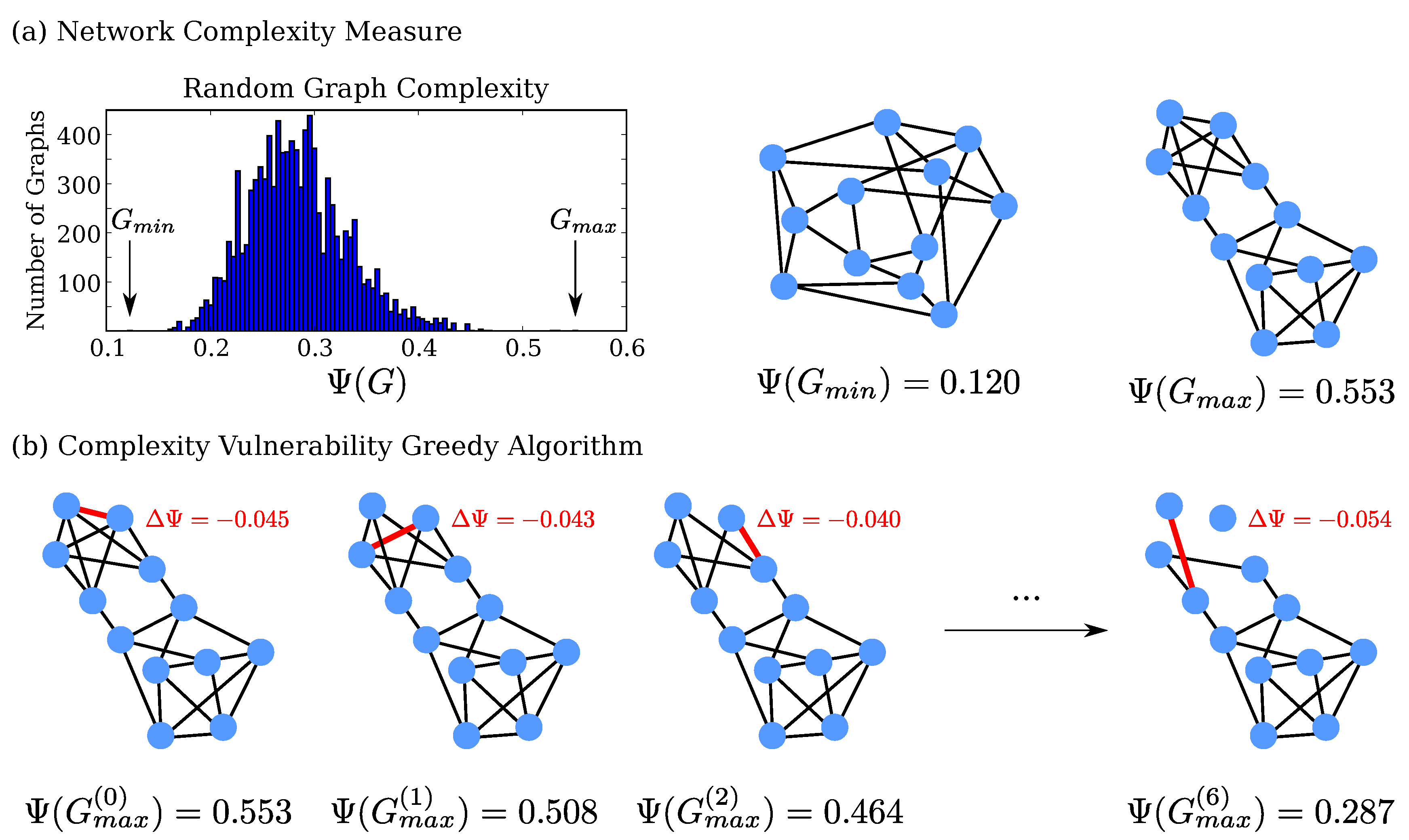
2.1. Investigation of Small, Random Networks

We begin our exploration of complexity/vulnerability analysis by considering graphs small enough to be easily visualized. We generated 10,000 random Erdős–Rényi networks, all of which had exactly 12 nodes each of degree four. This node count and degree were chosen heuristically such that the network would be small, but still large enough to allow for a very large number of possible connection schemes and complex structures. We investigate the complexity of these graphs by calculating the measure $\Psi (G)$, the aforementioned complexity measure developed in [5]. As detailed further in the Methods section, this measure is calculated as:

$$\Psi (G)=\frac{1}{N(N-1)}{\displaystyle \sum _i\sum _{j\ne i}}\max (K_i,K_j)m_{ij}(1-m_{ij}),$$

(1)

where the graph G consists of N nodes, $K_i$ is a measure of the complexity of the individual node i, and $m_{ij}$ is the mutual information between the connection patterns of nodes i and j. By construction, the summand vanishes when either $m_{ij}=0$ (as in random graphs) or $m_{ij}=1$ (when i and j are completely redundant). Complex networks reside between these two limiting cases.

Calculating $\Psi (G)$ for each of the small random graphs gives the distribution shown in Figure 1a. The very lowest and very highest values found were $\Psi (G_{\min })=0.120$ and $\Psi (G_{\max })=0.553$, respectively. The graphs corresponding to these extreme values are shown in Figure 1a.

In Figure 1b, we illustrate our greedy edge-elimination procedure, starting with the high-complexity graph $G_{\max }$. At each step, we individually delete every edge and calculate what the complexity of the graph would be without said edge. The edge causing the largest drop in Ψ (i.e., the highest magnitude of $\Delta \Psi$) is then chosen for deletion, giving the partially-deleted graph $G_{\max }^{(1)}$. This procedure is then iterated, recalculating each edge’s $\Delta \Psi$ within the partially deleted graph (i.e., $\Delta \Psi$ is re-calculated for all edges at each step).

It is interesting that the greedy procedure eliminates almost all of the edges from the pentagram-shaped structure before deleting any edges from the rest of the network. This suggests that the iterative elimination procedure may best reduce the network complexity by initially “attacking” a distinct structure within the network, rather than multiple, or more widely distributed structures. This suggests that we can usefully search for the property that unites the edges chosen for early elimination, as it may carry some structural significance. Specifically, we should consider any biophysiological significance associated with these edges; we suspect that the identified complex structures may be biophysically relevant, as complex network structures are capable of encoding biophysically important network dynamics [2,27].

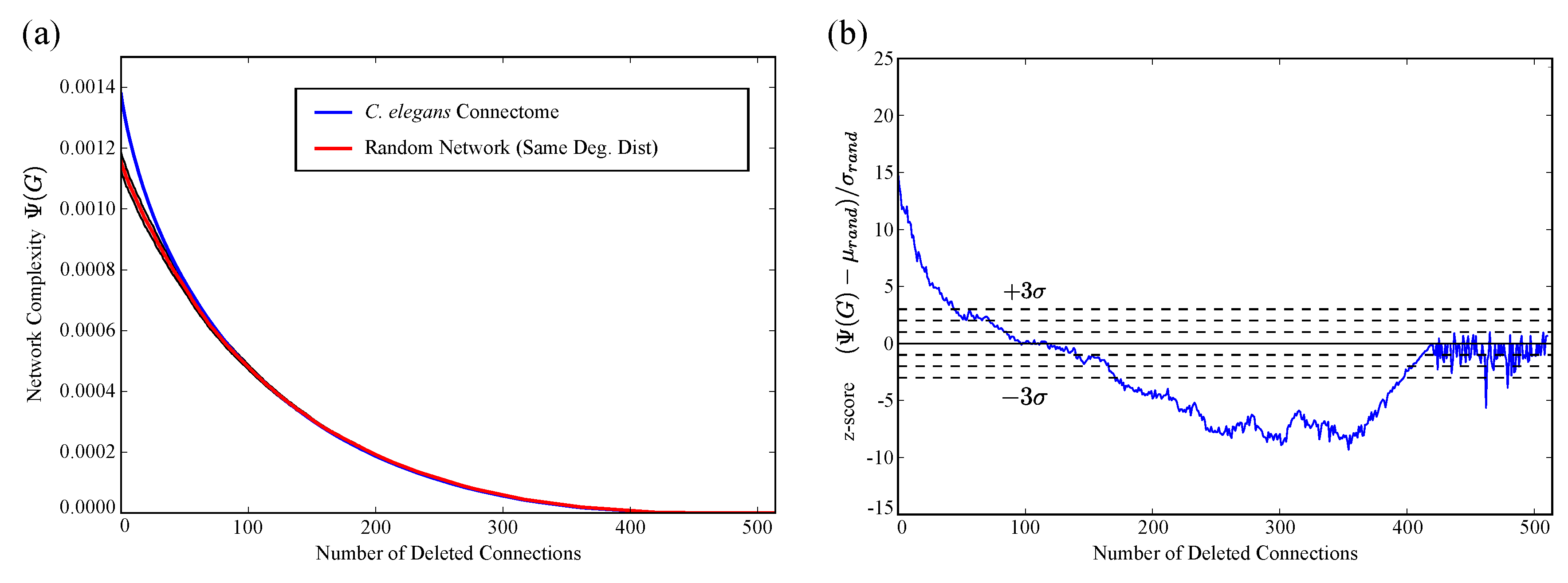
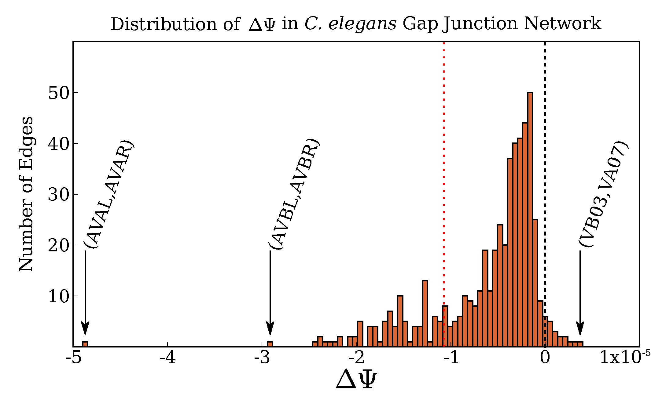
2.2. Application to C. Elegans Data

Using the C. elegans connectome data from Varshney et al. [7], we then proceed to apply the same edge-eliminating procedure to the C. elegans gap junction network. We focus here on the subnetwork of 253 somatic neurons which have both synaptic and gap junction connections. For this analysis, we ignore the weighting of each connection (i.e., number of gap junctions and gap junction connection strengths), simply labeling each pair of neurons as connected or unconnected. Thus, we represent the network as a binary, undirected graph with 253 nodes, connected by individual 514 edges.

Calculating Ψ for this network reveals that, by this measure, the C. elegans gap junction network is extraordinarily complex. We compare the actual gap junction network’s complexity to the complexity of 10,000 randomly-rewired networks, all of which have the exact same degree distribution (see Methods Section 4.5 for more information). Given its degree distribution, a random graph would have a complexity within an approximately normal distribution with a mean and standard deviation of $\Psi (G_{rand})=0.001173\pm 0.000015$. The neuron graph, however, has a complexity of $\Psi (G_{gap})=0.00143$, about 16.5 standard deviations above the random graph average. This distribution is plotted in comparison with the actual value in Figure 2.

Which edges are most responsible for this unusually high complexity? We use our edge deletion approach to explore this question. We begin by calculating $\Delta \Psi$ for every edge (i.e., the amount by which the network complexity would change were that edge deleted). The distribution of $\Delta \Psi$ values is shown in Figure 3. A few outliers are immediately apparent: the link between the command interneuron pair AVAL/AVAR, and the link between another command interneuron pair AVBL/AVBR. This suggests that the important biophysiological role of these neurons may be reflected in the relative complexity of their connection schemes. It is interesting that all edges to the left of the red dotted line implicate at least one interneuron.

We repeat the iterative, greedy edge-elimination procedure illustrated in Figure 1b, this time altering the C. elegans network. As it is intended to do, the procedure reduces the complexity of the network monotonically, eventually reducing the complexity to zero by deleting all edges. The complexity decay curve for the neuron graph is plotted in blue in Figure 4a. At each iteration, we generated 256 random graphs with the same modified degree distribution and plotted this distribution of random graph complexities in red.

This comparison is made clearer by converting the same data to z-scores (i.e., the number of standard deviations by which the C. elegans curve is away from the mean). This z-score curve is plotted in Figure 4b. As edges are progressively deleted, the complexity decays towards the randomly expected value, lying near the middle of the random range after about 100 deletions (about 25% of the edges). As edge deletion continues, however, the graph ultimately becomes much less complex than what one expects for a random graph. This suggests that the the graph consists of a low complexity component, connected with a smaller component connected to it that is responsible for the resulting excess complexity of the entire structure.

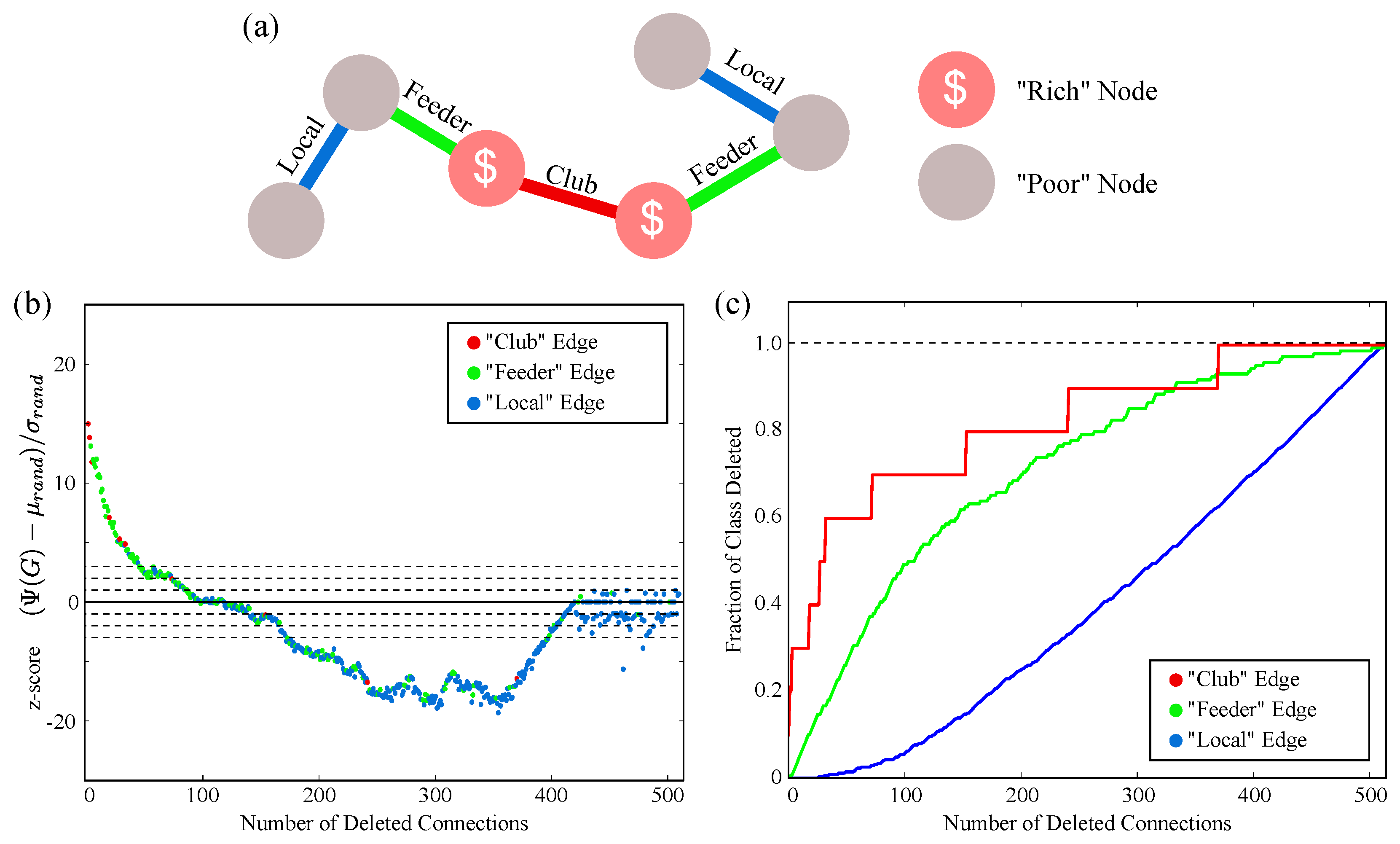
2.3. Complex Structure and the Rich Club

The discovery of a minority of edges that are particularly important to the complex structure of the network is reminiscent of the graph’s “rich club” property. Rich clubs within a graph are sets of high-degree nodes (the so-called “rich” nodes) which are highly interconnected. A rich node is more likely to connect with other rich nodes than one would expect at random, forming a highly-interconnected hub within the network that is important to the network’s function. This rich club structure appears in many complex networks [28] and helps to achieve a topologically desirable network (e.g., with high efficiency and centrality) for a relatively small wiring cost [16]. In neuroscience, a rich club architecture appears to be present in systems ranging from C. elegans to humans [17,18,19,20,21,22,23,24].

The C. elegans synaptic network was shown by Towlson et al. [24] to possess a rich club structure. We consider the set of neurons which they identified as the “rich club” due to their associated biological significance, though it should be noted that the gap junction network does not itself have the same rich club structure. Using the terminology of Towlson et al. [24], each edge in the graph can be classified as a “club” edge (if it connects two rich nodes), a “feeder” edge (if it connects a rich, high degree node to a poor node), or a “local” edge (if it connects two poor nodes). This is illustrated in Figure 5a. In Figure 5b, we label each edge in our deletion order according to these classes. This shows that the iterative procedure disproportionately targets club and feeder edges: out of the first 100 edge deletions, 19% are local, 74% are feeder, and 7% are club. By comparison, the intact network edges are about 69% local, 29% feeder, and 2% club. A ${\chi }^2$-test shows that the probability of randomly drawing as many feeder and club edges out of the network is less than $p<{10}^{-25}$; thus, the edge selection process heavily targets the rich club. This disproportionate targeting can be seen by looking at the percentage of each class that has been deleted at each iteration, as shown in Figure 5c.

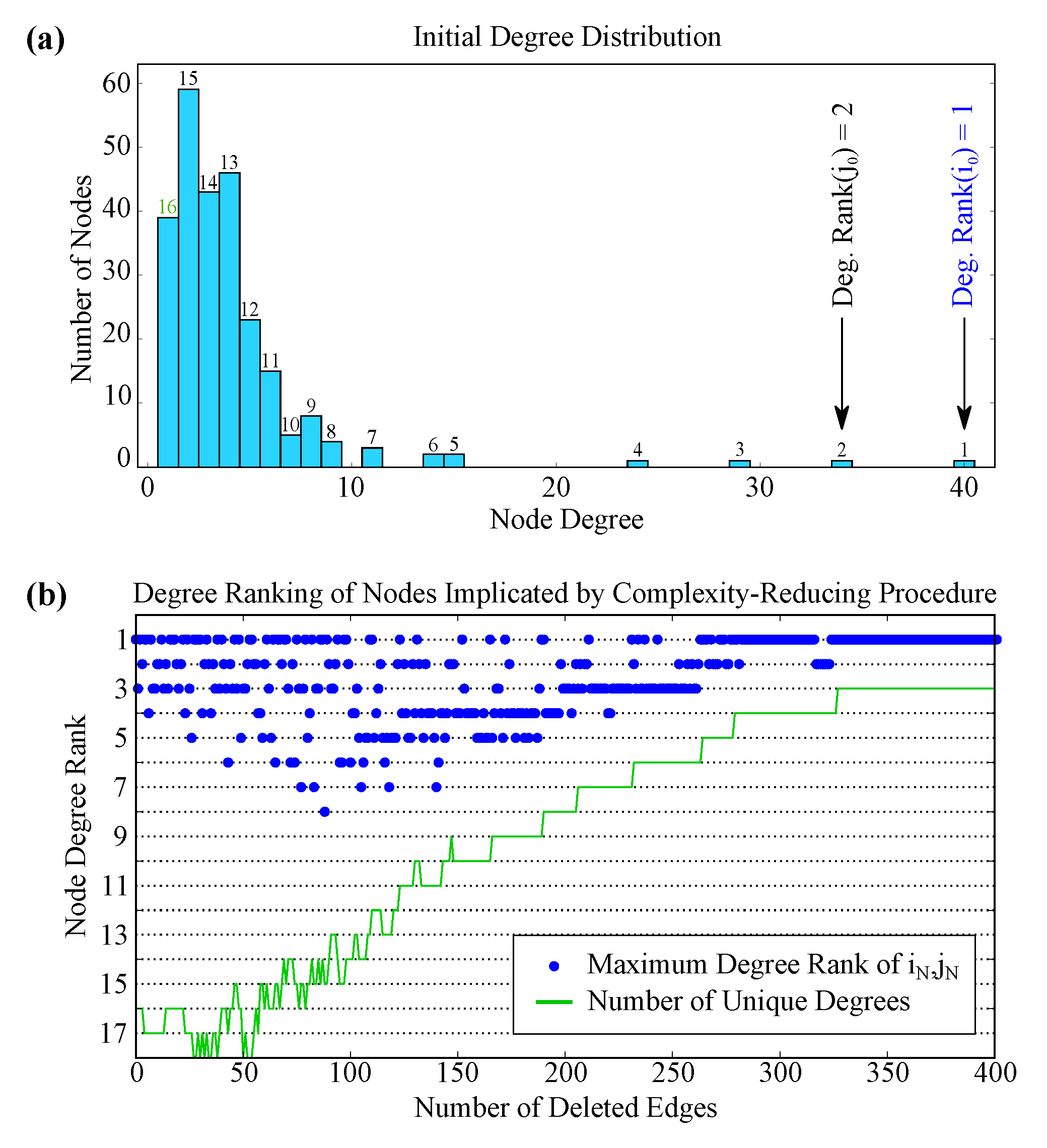
2.4. Complex Structure beyond Degree

The rich club is important to several complex topological properties of the network, but a node’s membership in the rich club is ultimately determined by its degree. The “rich club” nodes we consider are defined from their synaptic connectivity, and we are considering the gap junction network, but there is a positive correlation between a node’s gap junction degree and synaptic degree. It is therefore possible that this complexity-reduction procedure could yield a similar result (i.e., apparent targeting of the rich club nodes) if it were simply reducing the degrees of the highest-degree nodes. Figure 6a plots the initial degree distribution of the graph and shows that the first implicated edge $(i_0,j_0)$ is indeed between the first and second mostly highly-connected nodes. Could such a simple criterion explain these results, or is the procedure indeed targeting a more sophisticated structure?

Referring to Figure 1b, we suspect that the edge elimination order is not so trivial. After all, the procedure continued to target the pentagram-shaped structure even after those nodes had been trimmed to a very low degree. Indeed, we see similar results in the C. elegans network: Figure 6b shows how highly ranking the degree of the targeted nodes are at each step of the elimination procedure (i.e., whether or not the edge includes the 1st most highly connected node, the 2nd most highly connected node, and so on). Note that, at any given step, there are no more than 18 unique degrees (as there are many nodes sharing the same number of connections). For example, the second edge to be deleted is the edge between AVBR and AVBL, which have degrees 29 and 24, respectively. These are the 3rd and 4th highest degrees in the network at this point of the procedure, and so a blue marker is plotted at a node degree rank of 3. As can be seen in Figure 6b, many of the subsequent edge deletions do not implicate the most highly connected nodes. The highest-complexity edges are not simply determined by the degree of the implicated nodes.

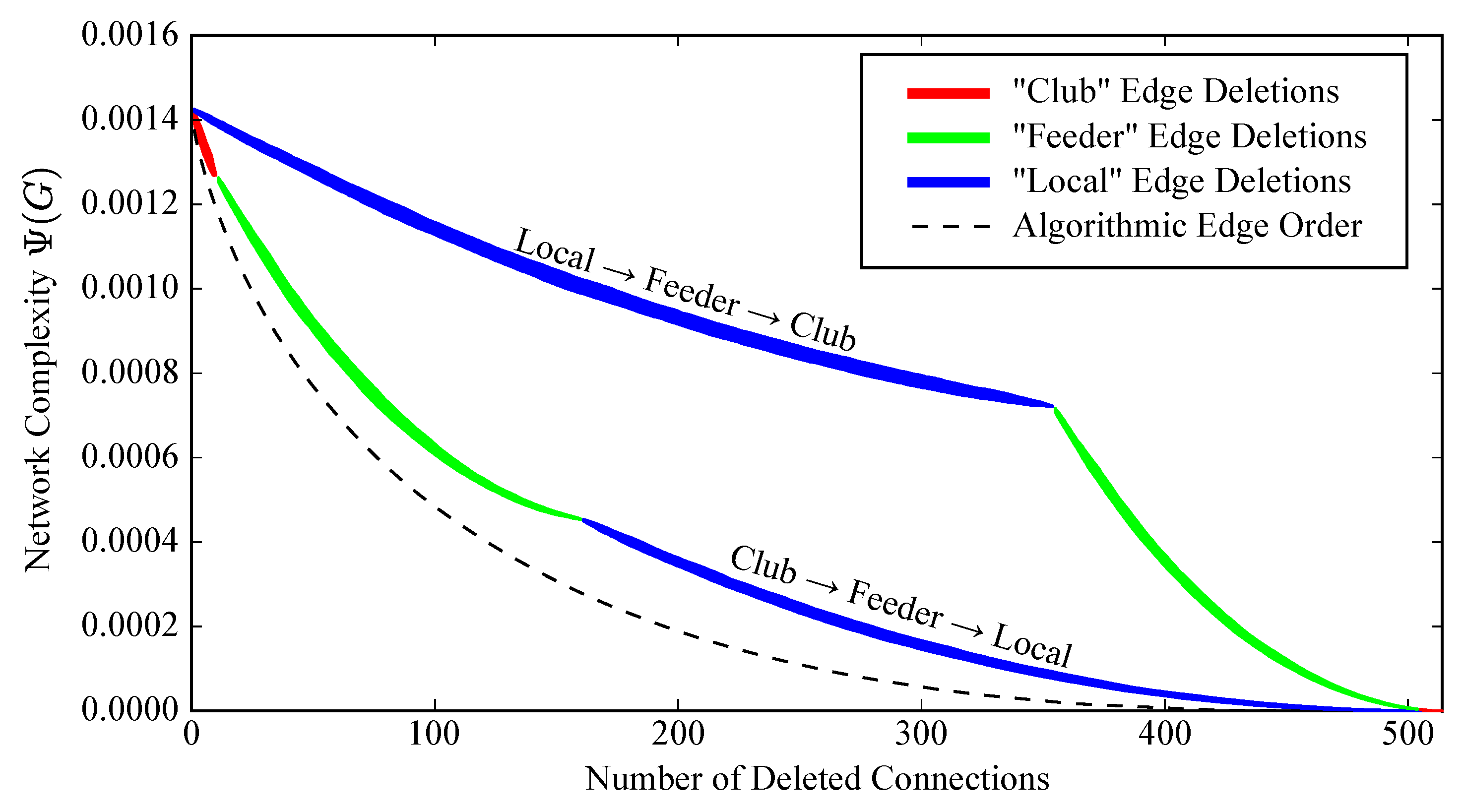
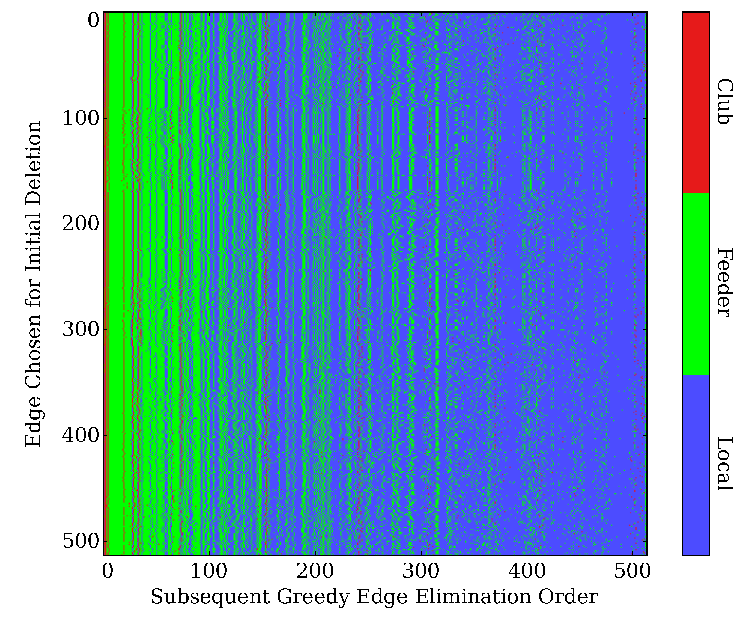
2.5. Robustness to Specific Elimination Order

How robust are these results to the specific order in which edges are eliminated? To address this, we conduct 50 trials in which we calculate the decay of $\Psi (G)$ when we delete all club edges in a random order, then delete all feeder edges in a random order, and then delete all local edges in a random order. The resulting distribution of complexity curves is shown in Figure 7. The random Club/Feeder/Local edge deletion orderings result in a smaller decrease in complexity than the algorithmically-determined ordering, which is unsurprising given the “greedy” nature of our edge-elimination procedure. However, the result is much more drastic when we conduct 50 trials in which we first delete the local edges, then the feeder edges, and then the club edges. This suggests that it is indeed appropriate to think of the network’s high complexity as being disproportionately caused by the club and feeder edges.

2.6. Robustness to Initial Edge Choice

We may similarly investigate the effect of choosing a different edge at the first deletion step. Consider again the example in Figure 1b, in which the iterative procedure initially targets nearly all of the edges within the upper pentagram-shaped structure. We interpreted this to mean that the pentagram-shaped structure was primarily responsible for the high complexity of the network. However, one could posit that the lower portion of the graph was similarly complex and that initially deleting an edge in the upper portion simply biased the iterative procedure towards targeting that portion of the graph. Does the initial edge deletion bias the procedure in this manner?

We directly investigated this possibility by repeating the analysis of Figure 5, but with an arbitrary edge chosen at the first deletion step (followed by the greedy iterative deletion procedure). This was repeated for all possible choices of initial edge deletions (i.e., for all 514 edges). When AVAL/AVAR is chosen initially (as in the full greedy procedure), the results are, of course, identical to the previous results. For all of the other 513 initializations, however, the greedy procedure chooses AVAL/AVAR as the very next edge to be deleted. Furthermore, the procedure continues to target club/feeder edges in largely the same manner. Figure 8 shows the order in which edges of each class are deleted for all possible initial edge choices. Despite minor variations in edge ordering, the order in which edges are targeted by the greedy procedure appears to be largely robust to the initial edge choice, and the disproportionate targeting of club/feeder edges does not depend upon this initialization.

3. Discussion

This study shows that the C. elegans neuron gap–junction network is vastly more complex than one would expect at random given its degree distribution. Expanding the concept of vulnerability analysis, we analyzed the complexity vulnerability of the graph and used an iterative procedure to successively eliminate edges based upon how much each deletion reduced graph complexity. After many edge deletions, we were left with a graph much less complex than an equivalent random graph. This suggests that the majority of the graph consists of a low complexity component that can be described fairly simply, and a subset of edges, which is responsible for the excess complexity of the network. This complexity-causing set of edges belongs disproportionately to the neurons which are members of the associated synaptic network’s previously-identified rich club.

The fact that the procedure reduces the graph to one with a remarkably low complexity raises interesting questions concerning the topology of graphs. Many graphs, particularly in biology and neuroscience and including the C. elegans neuronal network, are rather well-described by a collection of over-represented motifs [7,29,30,31]. A common view of neuronal networks, as consisting of a highly structured graph of repeated motifs with the repetitive structure violated by important hub neurons, is interesting to compare with the results in Figure 4. Is the iterative procedure simply stripping away these hub structures to leave a simple, highly-repetitive core? Given that this complexity measure disappears when the mutual information between nodes approaches 1, it is plausible that particularly motif-heavy graphs, consisting of sets of nodes having similar connectivity patterns/high mutual information, may be classified as having a particularly low complexity by this measure. The exact relationship between motif structures, symmetry and symmetry-breaking and their effects upon network complexity measures deserves a deeper theoretical investigation, which will be the subject of future work.

These results also suggest that future work should investigate the broader range of structural properties to which this complexity measure is sensitive. It is important to note that this procedure does not simply identify rich-club structure; recall that we consider the “rich club” set of neurons due to its previously-identified importance, but this set is defined from the synaptic network, not the gap junction network, which lacks such structure. What functionally relevant structures does this approach reveal, and what are the associated topological properties? For example, one could consider the change in average betweenness centrality as nodes are iteratively deleted. Initially, the network has an average betweenness which is a factor of about 1.29 higher than that of a random graph (with the same degree distribution). After 40 deletions, this factor is reduced to 1.22. This small reduction does not appear to explain the large reduction in relative complexity over the same range (as seen in Figure 4). Other preliminary work has been similarly inconclusive, suggesting that the relationship between complexity and other topological measures is nontrivial. The more general relationship between network complexity and various other global topological properties of the network is beyond the scope of this paper, but the subject of future work.

How would the identified structures differ if one uses a different quantification of network complexity? There is no universally recognized quantification of network complexity, and many such measures exist [3,4,32,33]. Furthermore, the Ψ measure is inherently dependent only on pairwise measures of connectivity in the sense that it is a sum over pairs of mutual information between nodes based on their connectivity. Measures that include higher numbers of nodes and their informational interdependence might reveal other features [23,32,33]. It should be possible to perform a similar deconstruction procedure using other measures, which may distinguish different features and could prove useful both as a tool for the exploration of the structure of networks and for illuminating the differences between the measures themselves.

Further development of network complexity quantification and exploration of different measures could incorporate information which we have ignored thus far in our analysis. Since we used an undirected network complexity measure, we focused upon the undirected gap junction network. However, the directed synaptic network is also vitally important, and the method can be modified to incorporate directed connections. Similarly, we consider the unweighted binary graph, ignoring edge-weighting data such as the number of gap junctions between each node. Future analysis could make use of such information, perhaps by using previously-developed extensions of this complexity measure to include multiple edge types [6].

In spite of these current limitations, this study strongly suggests that quantifying a network’s global complexity, performing vulnerability analysis using this complexity measure, and then iteratively eliminating edges based upon their vulnerability at each step is a useful direction for identifying physiologically important structures within complex graphs. Such methods are increasingly important as increasingly large and difficult-to-comprehend neuronal networks are measured by the burgeoning field of connectomics [34,35,36]. In a real network, the interaction between the structural features, the behavior and flexibility of the network function, the vulnerability to damage and the costs of wiring the networks are fundamental. The trade-offs can only be fully understood by careful quantitative analysis of the kind begun here. Given the potentially scale-invariant nature of neuroscience networks [24], the architectural principles we infer from these complex networks may yield broader design insights into the function and structure of nervous system networks.

4. Materials and Methods

4.1. Network Complexity $\Psi (G)$

The graph complexity measure $\Psi (G)$ is an information theoretic measure with a basis in the Kolmogorov complexity and was introduced and explored for undirected binary graphs by Sakhanenko and Galas [5]. Consider an undirected binary graph with N nodes, characterized by a symmetric adjacency matrix $A=\left\{a_{ij}\right\}$, where $a_{ij}=1$ if nodes i and j are connected, and $a_{ij}=0$ if they are not. The measure is based on a Shannon-like description of information, such that the fundamental properties of a node are its connection probabilities. We denote the connection probability of node i by:

$$p_i(1)=\frac{1}{N-1}{\displaystyle \sum _{j\ne i}}{a}_{ij}.$$

(2)

Similarly, the disconnection probability is given by:

$$p_i(0)=\frac{1}{N-1}{\displaystyle \sum _{j\ne i}}(1-a_{ij}).$$

(3)

The complexity of an individual node is then given by:

$$K_i={\displaystyle \sum _{a=0}^1}{p}_i(a){\log }_2(p_i(a)).$$

(4)

We can then calculate the mutual information between two nodes i an j:

$$m_{ij}={\displaystyle \sum _{a=0}^1\sum _{b=0}^1}{p}_{ij}(a,b){\log }_2\left(\frac{p_{ij}(a,b)}{p_i(a)p_j(b)}\right).$$

(5)

The graph complexity Ψ can then be calculated from the mutual informations and individual node complexities:

$$\Psi =\frac{1}{N(N-1)}{\displaystyle \sum _i\sum _{j\ne i}}\max (K_i,K_j)m_{ij}(1-m_{ij}).$$

(6)

Note that the summands will disappear when either $m_{ij}=0$ or $m_{ij}=1$. The former case is when the connectivity patterns of the two nodes contain no information about the other, as is the case of infinite random graphs. The latter case occurs when two nodes carry perfect information about the other, as is the case with completely connected or completely disconnected graphs. Thus, the graph complexity will disappear in both of these limiting cases.

4.2. $\Delta \Psi (G)$ and Iterative Edge Removal

Our greedy algorithm for complexity vulnerability analysis consists of iteratively deleting the graph edges whose deletions cause the largest reduction in graph complexity. That is, for an initial adjacency matrix $A^{(0)}$, we consider all one-edge deletions and recalculate the resulting Ψ, finding the edge $(i_1,j_1)$ which causes the largest reduction in Ψ when deleted. We refer to the new adjacency matrix, with the single edge deletion, as $A^{(1)}$. We then repeat this process with $A^{(1)}$ to identify $(i_2,j_2)$. This is repeated until all N edges are deleted, yielding an edge deletion order $e=\{(i_1,j_1),(i_2,j_2),(i_3,j_3),\dots ,(i_N,j_N)\}$.

For notational purposes, we define a matrix $\Delta (i,j)$ which is equal to one at entry $(i,j)$ and is zero for all other entries. That is,

$$\Delta {(i^{\prime },j^{\prime })}_{ij}=\left\{\begin{array}{cc}1,\hfill & \mathrm{if}(i,j)=(i^{\prime },j^{\prime }),\hfill \\ 0,\hfill & \mathrm{otherwise}.\hfill \end{array}\right.$$

(7)

This allows us to write the adjacency matrix with a single edge deletion at $(i^{\prime },j^{\prime })$ as $A-\Delta (i^{\prime },j^{\prime })$. We select the first edge to delete by calculating:

$$(i_0,j_0)=\underset{i,j}{\mathrm{argmin}}[\Psi (A^{(0)}-\Delta (i,j))].$$

(8)

That is, we choose the indices of the edge deletion resulting in the graph with the least complexity. We can write the resulting adjacency matrix as:

$$A^{(1)}=A^{(0)}-\Delta (i_0,j_0).$$

(9)

We write the corresponding change in complexity as:

$$\Delta {\Psi }^{(1)}=\Psi (A^{(1)})-\Psi (A^{(0)}).$$

(10)

This process is repeated iteratively until all edges are deleted. At the nth edge deletion we may write:

$$(i_n,j_n)=\underset{i,j}{\mathrm{argmin}}[\Psi (A^{(n)}-\Delta (i,j))],$$

(11)

$$A^{(n+1)}=A^{(n)}-\Delta (i_n,j_n).$$

(12)

4.3. Illustrative Example: 12 Nodes of Four Degrees

Using the Python package graph-tool [37], we generated 10,000 random Erdős–Rényi graphs, all consisting of 12 nodes which all have degree four. We calculated Ψ for all of these 10,000 graphs, giving the distribution seen in Figure 1a. We then applied the iterative edge-removal procedure from Section 4.2 to the random graph which had the highest value of Ψ. This gave the edge removal ordering as partially visualized in Figure 1b.

4.4. The C. Elegans Connectome

The C. elegans neuronal network consists of 302 neurons connected via both a directed synaptic network (with 6393 synapses) and undirected gap junction network (with 890 gap junctions) [7]. The bulk of these neurons, 282 out of 302, belong to the somatic nervous system. We use the connectivity data for the giant component of the somatic nervous system, consisting of 279 neurons, as provided by Varshney et al. [7], who consolidated and updated earlier connectome measurements [38,39,40].

Since this work focuses on the structure of undirected graphs, our analysis is of the gap junction network. All of the 279 neurons within the network are connected synaptically, but many lack gap junctions entirely. We eliminate the neurons that have no gap junction connections, leaving the 253 somatic neurons with both synaptic and gap junction connections. Many nodes share multiple connections, but we simplify our analysis by considering the unweighted network: $a_{ij}=1$ if nodes i and j have one or more gap junction connections, or $a_{ij}=0$ if they have no gap junction connections. Thus, our adjacency matrix $A^{(0)}$ consists of 253 nodes connected by 514 binary edges.

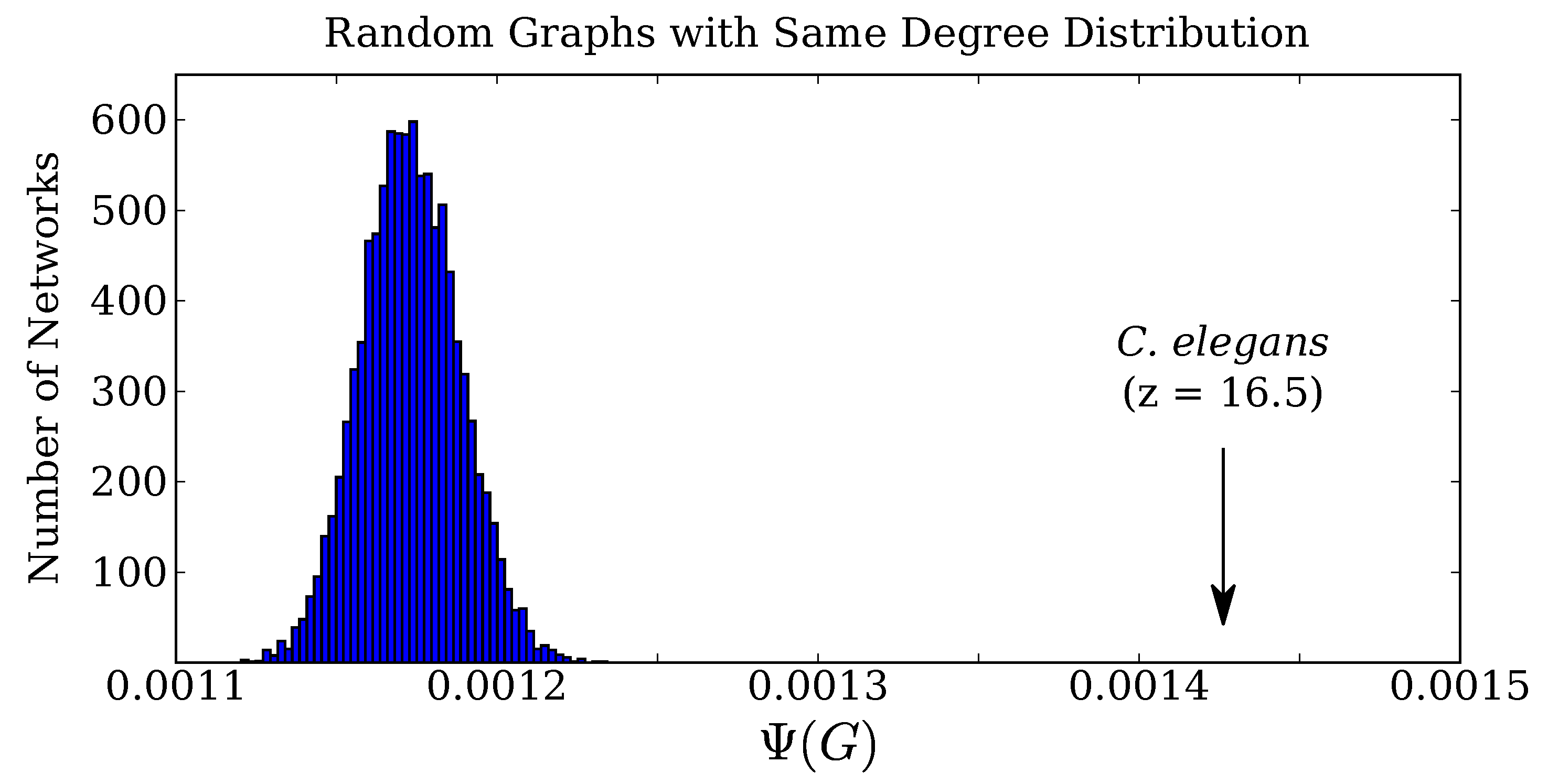
4.5. Comparison of C. elegans to Random Connectivity

To compare the complexity of the actual Connectome against what we might expect at random, we use the random_rewire function included within the Python package graph-tool [37], selecting the “uncorrelated” rewiring model. This procedure is described in the graph-tool documentation and can be summarized as follows: for each edge $(i,j)$, the algorithm randomly selects a second edge $(i^{\prime },j^{\prime })$. It then attempts to swap the target of each edge, such that the edges would then become $(i,j^{\prime })$ and $(i^{\prime },j)$. This swap is rejected if it would result in parallel edges or self-loops. This swapping procedure is repeated for all edges $(i,j)$ within the graph. This rewires a graph to randomize connections while preserving the exact degree sequence.

For the distribution of Figure 2, we generated 10,000 randomly-rewired graphs with the same degree distribution as the C. elegans gap junction network, yielding the displayed distribution with a mean and standard deviation of $\Psi (G_{rand})=0.001173\pm 0.000015$. As we iteratively eliminated edges, we wished to continue comparing the reduced complexity against what we would expect at random. At each step n, we therefore randomly rewired the partially deleted graph $A^{(n)}$ to generate 256 graphs with the same (partially deleted) degree distribution.

4.6. C. elegans Rich Club

The “rich club” is defined by the rich club coefficient $\Phi (k)$, which is defined by the connection probability between nodes of degree greater than k. For some degree k, define $N_{>k}$ as the number of nodes with degree greater than k, and $M_{>k}$ as the number of connections between said nodes. The rich club coefficient is then just the ratio between the actual number of connections $M_{>k}$ and the number of possible connections [24,28,41]:

$$\Phi (k)=\frac{2M_{>k}}{N_{>k}(N_{>k}-1).}$$

(13)

Towlson et al. [24] found that the C. elegans Connectome has a significant rich club coefficient for degrees $35\le k\le 73$, which implicates the following 11 nodes as belonging to the rich club: AVAL/R, AVBL/R, AVDL/R, AVEL/R, PVCL/R, and DVA. It is important to note that this is the set of neurons which we use as the “rich club” of the network, and we do not do any re-calculation of the rich club based on our particular graph; Towlson calculates the rich club set from a binary form of the synaptic network, whereas we consider a binary form of the gap junction network. We refer to this set of neurons due to its known biological significance.

References

- Sporns, O. The Non-Random Brain: Efficiency, Economy, and Complex Dynamics. Front. Comput. Neurosci. 2011, 5. [Google Scholar] [CrossRef] [PubMed]
- Gollo, L.L.; Zalesky, A.; Hutchison, R.M.; van den Heuvel, M.; Breakspear, M. Dwelling quietly in the rich club: Brain network determinants of slow cortical fluctuations. Philos. Trans. R. Soc. Lond. B Biol. Sci. 2015, 370. [Google Scholar] [CrossRef] [PubMed]
- Dehmer, M.; Barbarini, N.; Varmuza, K.; Graber, A. A Large Scale Analysis of Information-Theoretic Network Complexity Measures Using Chemical Structures. PLoS ONE 2009, 4, e8057. [Google Scholar] [CrossRef] [PubMed]
- Emmert-Streib, F.; Dehmer, M. Exploring Statistical and Population Aspects of Network Complexity. PLoS ONE 2012, 7, e34523. [Google Scholar] [CrossRef] [PubMed]
- Sakhanenko, N.A.; Galas, D.J. Complexity of Networks I: The SetComplexity of Binary Graphs. Complexity 2011, 17, 51–64. [Google Scholar] [CrossRef]
- Ignac, T.M.; Sakhanenko, N.A.; Galas, D.J. Complexity of Networks II: The Set Complexity of Edge-colored Graphs. Complexity 2012, 17, 23–36. [Google Scholar] [CrossRef]
- Varshney, L.R.; Chen, B.L.; Paniagua, E.; Hall, D.H.; Chklovskii, D.B. Structural Properties of the Caenorhabditis elegans Neuronal Network. PLoS Comput. Biol. 2011, 7, e1001066. [Google Scholar] [CrossRef] [PubMed]
- Chalfie, M.; Sulston, J.E.; White, J.G.; Southgate, E.; Thomson, J.N.; Brenner, S. The neural circuit for touch sensitivity in Caenorhabditis elegans. J. Neurosci. 1985, 5, 956–964. [Google Scholar] [PubMed]
- Sawin, E. Genetic and Cellular Analysis of Modulated Behaviors in Caenorhabditis elegans. Ph.D. Thesis, Massachusetts Institute of Technology, Cambridge, MA, USA, 1996. [Google Scholar]
- Sawin, E.R.; Ranganathan, R.; Horvitz, H.R. C. elegans locomotory rate is modulated by the environment through a dopaminergic pathway and by experience through a serotonergic pathway. Neuron 2000, 26, 619–631. [Google Scholar] [CrossRef]
- Gray, J.M.; Hill, J.J.; Bargmann, C.I. A circuit for navigation in Caenorhabditis elegans. Proc. Natl. Acad. Sci. USA 2005, 102, 3184–3191. [Google Scholar] [CrossRef] [PubMed]
- Liu, K.S.; Sternberg, P.W. Sensory regulation of male mating behavior in Caenorhabditis elegans. Neuron 1995, 14, 79–89. [Google Scholar] [CrossRef]
- Macosko, E.Z.; Pokala, N.; Feinberg, E.H.; Chalasani, S.H.; Butcher, R.A.; Clardy, J.; Bargmann, C.I. A hub-and-spoke circuit drives pheromone attraction and social behaviour in C. elegans. Nature 2009, 458, 1171–1175. [Google Scholar] [CrossRef] [PubMed]
- Bany, I.A.; Dong, M.Q.; Koelle, M.R. Genetic and cellular basis for acetylcholine inhibition of Caenorhabditis elegans egg-laying behavior. J. Neurosci. 2003, 23, 8060–8069. [Google Scholar] [PubMed]
- Hardaker, L.A.; Singer, E.; Kerr, R.; Zhou, G.; Schafer, W.R. Serotonin modulates locomotory behavior and coordinates egg-laying and movement in Caenorhabditis elegans. J. Neurobiol. 2001, 49, 303–313. [Google Scholar] [CrossRef] [PubMed]
- Bassett, D.S.; Greenfield, D.L.; Meyer-Lindenberg, A.; Weinberger, D.R.; Moore, S.W.; Bullmore, E.T. Efficient physical embedding of topologically complex information processing networks in brains and computer circuits. PLoS Comput. Biol. 2010, 6, e1000748. [Google Scholar] [CrossRef] [PubMed]
- Van den Heuvel, M.P.; Sporns, O. Rich-Club Organization of the Human Connectome. J. Neurosci. 2011, 31, 15775–15786. [Google Scholar] [CrossRef] [PubMed]
- Bullmore, E.; Sporns, O. The economy of brain network organization. Nat. Rev. Neurosci. 2012, 13, 336–349. [Google Scholar] [CrossRef] [PubMed]
- Harriger, L.; van den Heuvel, M.P.; Sporns, O. Rich club organization of macaque cerebral cortex and its role in network communication. PLoS ONE 2012, 7, e46497. [Google Scholar] [CrossRef] [PubMed]
- Ball, G.; Aljabar, P.; Zebari, S.; Tusor, N.; Arichi, T.; Merchant, N.; Robinson, E.C.; Ogundipe, E.; Rueckert, D.; Edwards, A.D.; et al. Rich-club organization of the newborn human brain. Proc. Natl. Acad. Sci. USA 2014, 111, 7456–7461. [Google Scholar] [CrossRef] [PubMed]
- Schroeter, M.S.; Charlesworth, P.; Kitzbichler, M.G.; Paulsen, O.; Bullmore, E.T. Emergence of rich-club topology and coordinated dynamics in development of hippocampal functional networks in vitro. J. Neurosci. 2015, 35, 5459–5470. [Google Scholar] [CrossRef] [PubMed]
- Nigam, S.; Shimono, M.; Ito, S.; Yeh, F.C.; Timme, N.; Myroshnychenko, M.; Lapish, C.C.; Tosi, Z.; Hottowy, P.; Smith, W.C.; et al. Rich-club organization in effective connectivity among cortical neurons. J. Neurosci. 2016, 36, 670–684. [Google Scholar] [CrossRef] [PubMed]
- Pedersen, M.; Omidvarnia, A. Further Insight into the Brain’s Rich-Club Architecture. J. Neurosci. 2016, 36, 5675–5676. [Google Scholar] [CrossRef] [PubMed]
- Towlson, E.K.; Vértes, P.E.; Ahnert, S.E.; Schafer, W.R.; Bullmore, E.T. The Rich Club of the C. elegans Neuronal Connectome. J. Neurosci. 2013, 33, 6380–6387. [Google Scholar] [CrossRef] [PubMed]
- Kunert, J.; Shlizerman, E.; Kutz, J.N. Low-dimensional functionality of complex network dynamics: Neurosensory integration in the Caenorhabditis elegans connectome. Phys. Rev. E 2014, 89, 052805. [Google Scholar] [CrossRef] [PubMed]
- Kim, S.; Kim, H.; Kralik, J.D.; Jeong, J. Vulnerability-Based Critical Neurons, Synapses, and Pathways in the Caenorhabditis elegans Connectome. PLoS Comput. Biol. 2016, 12, e1005084. [Google Scholar] [CrossRef] [PubMed]
- Hu, Y.; Brunton, S.L.; Cain, N.; Mihalas, S.; Kutz, J.N.; Shea-Brown, E. Feedback through graph motifs relates structure and function in complex networks. arXiv, 2016; arXiv:1605.09073. [Google Scholar]
- Colizza, F.; Flammini, A.; Serrano, M.; Vespignani, A. Detecting rich-club ordering in complex networks. Nat. Phys. 2006, 2, 110–115. [Google Scholar] [CrossRef]
- Milo, R.; Shen-Orr, S.; Itzkovitz, S.; Kashtan, N.; Chklovskii, D.; Alon, U. Network Motifs: Simple Building Blocks of Complex Networks. Science 2002, 298, 824–827. [Google Scholar] [CrossRef] [PubMed]
- Sporns, O.; Kötter, R. Motifs in Brain Networks. PLoS Biol. 2004, 2, e369. [Google Scholar] [CrossRef] [PubMed]
- Qian, J.; Hintze, A.; Adami, C. Colored Motifs Reveal Computational Building Blocks in the C. elegans Brain. PLoS ONE 2011, 6, e17013. [Google Scholar] [CrossRef] [PubMed]
- Galas, D.J.; Sakhanenko, N.A.; Skupin, A.; Ignac, T. Describing the Complexity of Systems: Multivariable “Set Complexity” and the Information Basis of Systems Biology. J. Comput. Biol. 2014, 21, 118–140. [Google Scholar] [CrossRef] [PubMed]
- Sakhanenko, N.; Galas, D. Biological Data Analysis as an Information Theory Problem: Multivariable Dependence Measures and the Shadows Algorithm. J. Comput. Biol. 2015, 22, 1005–1024. [Google Scholar] [CrossRef] [PubMed]
- Bohland, J.W.; Wu, C.; Barbas, H.; Bokil, H.; Bota, M.; Breiter, H.C.; Cline, H.T.; Doyle, J.C.; Freed, P.J.; Greenspan, R.J.; et al. A Proposal for a Coordinated Effort for the Determination of Brainwide Neuroanatomical Connectivity in Model Organisms at a Mesoscopic Scale. PLoS Comput. Biol. 2009, 5, e1000334. [Google Scholar] [CrossRef] [PubMed]
- Chiang, A.S.; Lin, C.Y.; Chuang, C.C.; Chang, H.M.; Hsieh, C.H.; Yeh, C.W.; Shih, C.T.; Wu, J.J.; Wang, G.T.; Chen, Y.C.; et al. Three-Dimensional Reconstruction of Brain-wide Wiring Networks in Drosophila at Single-Cell Resolution. Curr. Biol. 2011, 21, 1–11. [Google Scholar] [CrossRef] [PubMed]
- Oh, S.; Harris, J.; Ng, L.; Winslow, B.; Cain, N.; Mihalas, S.; Wang, Q.; Lau, C.; Kuan, L.; Henry, A.; et al. A mesoscale connectome of the mouse brain. Nature 2014, 508, 207–214. [Google Scholar] [CrossRef] [PubMed]
- Peixoto, T.P. The graph-tool python library. Figshare 2014. [Google Scholar] [CrossRef]
- White, J.G.; Southgate, E.; Thomson, J.N.; Brenner, S. The structure of the nervous system of the nematode Caenorhabditis elegans. Philos. Trans. R. Soc. Lond. B Biol. Sci. 1986, 314. [Google Scholar] [CrossRef]
- Hall, D.H.; Russell, R.L. The posterior nervous system of the nematode Caenorhabditis elegans: Serial reconstruction of identified neurons and complete pattern of synaptic interactions. J. Neurosci. 1991, 11, 1–22. [Google Scholar] [PubMed]
- Durbin, R. Studies on the Development and Organisation of the Nervous System of Caenorhabditis elegans. Ph.D. Thesis, University of Cambridge, Cambridge, UK, 1987. [Google Scholar]
- Zhou, S.; Mondragon, R. The rich-club phenomenon in the internet topology. IEEE Commun. Lett. 2004, 8, 180–182. [Google Scholar] [CrossRef]
© 2017 by the authors. Licensee MDPI, Basel, Switzerland. This article is an open access article distributed under the terms and conditions of the Creative Commons Attribution (CC BY) license ( http://creativecommons.org/licenses/by/4.0/).
Share and Cite
Kunert-Graf, J.M.; Sakhanenko, N.A.; Galas, D.J. Complexity and Vulnerability Analysis of the C. Elegans Gap Junction Connectome. Entropy 2017, 19, 104. https://doi.org/10.3390/e19030104
Kunert-Graf JM, Sakhanenko NA, Galas DJ. Complexity and Vulnerability Analysis of the C. Elegans Gap Junction Connectome. Entropy. 2017; 19(3):104. https://doi.org/10.3390/e19030104
Chicago/Turabian StyleKunert-Graf, James M., Nikita A. Sakhanenko, and David J. Galas. 2017. "Complexity and Vulnerability Analysis of the C. Elegans Gap Junction Connectome" Entropy 19, no. 3: 104. https://doi.org/10.3390/e19030104
APA StyleKunert-Graf, J. M., Sakhanenko, N. A., & Galas, D. J. (2017). Complexity and Vulnerability Analysis of the C. Elegans Gap Junction Connectome. Entropy, 19(3), 104. https://doi.org/10.3390/e19030104