Article

Automated Detection of Paroxysmal Atrial Fibrillation Using an Information-Based Similarity Approach

1
School of Biological Sciences & Medical Engineering, Southeast University, Nanjing 210000, China
2
Departments of Computer Science and Biology, Emory University, Atlanta, GA 30322, USA
3
Department of Industrial Engineering and Management, Yuan Ze University, Taoyuan 320, Taiwan
4
Industrial Management Department, National Taiwan University of Science and Technology, Taipei 100, Taiwan
5
Center for Dynamical Biomarkers, Beth Israel Deaconess Medical Center/Harvard Medical School, Boston, MA 02215, USA
*
Authors to whom correspondence should be addressed.
Entropy 2017, 19(12), 677; https://doi.org/10.3390/e19120677
Submission received: 10 October 2017 / Revised: 20 November 2017 / Accepted: 8 December 2017 / Published: 10 December 2017
(This article belongs to the Special Issue Information Theory Applied to Physiological Signals)

Abstract

:
Atrial fibrillation (AF) is an abnormal rhythm of the heart, which can increase heart-related complications. Paroxysmal AF episodes occur intermittently with varying duration. Human-based diagnosis of paroxysmal AF with a longer-term electrocardiogram recording is time-consuming. Here we present a fully automated ensemble model for AF episode detection based on RR-interval time series, applying a novel approach of information-based similarity analysis and ensemble scheme. By mapping RR-interval time series to binary symbolic sequences and comparing the rank-frequency patterns of m-bit words, the dissimilarity between AF and normal sinus rhythms (NSR) were quantified. To achieve high detection specificity and sensitivity, and low variance, a weighted variation of bagging with multiple AF and NSR templates was applied. By performing dissimilarity comparisons between unknown RR-interval time series and multiple templates, paroxysmal AF episodes were detected. Based on our results, optimal AF detection parameters are symbolic word length m = 9 and observation window n = 150, achieving 97.04% sensitivity, 97.96% specificity, and 97.78% overall accuracy. Sensitivity, specificity, and overall accuracy vary little despite changes in m and n parameters. This study provides quantitative information to enhance the categorization of AF and normal cardiac rhythms.

1. Introduction

Atrial fibrillation (AF), the most common sustained cardiac arrhythmia, is an abnormal heart rhythm characterized by rapid and irregular beating of the atria [1]. The disease is associated with an increased risk of heart failure, dementia, stroke and other heart-related complications [2]. Paroxysmal AF (PAF), also termed intermittent AF, is defined as an episode of AF that terminates spontaneously or with intervention in less than seven days [3]. The frequency of PAF is uncertain, because previous studies have suggested that a majority of these episodes are asymptomatic [4,5], including some that may last more than 48 h [4]. Experienced clinicians can identify AF patterns by visual inspection of the electrocardiogram (ECG) chart. However, due to the paroxysmal nature of the onset and termination of PAF in certain patients, human-based diagnosis of AF is usually time consuming when using a longer-term ECG recording such as a Holter or event recorder. Therefore, an automated, computerized AF detector may provide timely diagnosis and have substantial clinical utility.
It is challenging to implement diagnostic ECG waveform criteria for AF into a computerized algorithm, partly due to the difficulty of quantifying P-waves (and their absence) and that cardiac inter-beat intervals, i.e., RR intervals, follow no repetitive patterns. One feasible approach is to identify the presence of irregular ventricular rhythm during AF episodes based on analysis of RR intervals [6,7,8,9,10,11,12,13,14,15,16,17,18,19,20,21,22,23,24,25]. Moody and Mark [11] showed that the Markov process model for the AF detection is equivalent to determining the arithmetic mean of a series scores based on the RR interval sequence. Tateno and Glass applied standard density histograms of the RR and ∆RR intervals to detect the onset and termination of AF using standard coefficients of variation and the Kolmogorov–Smirnov test [12]. Kikillus, et al. [13] and Babaeizadeh, et al. [14] applied Markov modeling technique to identify AF. Lian, et al. [15] developed an AF detector with its basis centered on the Map of RR intervals versus change of RR intervals. Huang, et al. [16] utilized a histogram of ΔRRn and standard deviation analysis. Parvaresh, et al. [17] evaluated three classifiers for AF screening by using autoregressive modeling. Dash, et al. [18] proposed the randomness-variability-complexity approach. Lee, et al. [19] introduced the time-varying coherence approach. Petrenas, et al. [20] applied the low-complexity approach. Zhou, et al. [21,22] proposed the symbolic dynamics approach. Additionally, the entropy and heart rate dynamics approaches were also used in many studies [23,24,25,26]. Other studies of AF detections are based on the analysis of the probability density or autocorrelation function of the RR interval series during AF [27,28,29].
Studies have demonstrated that physiologic systems generate complex fluctuations in their output signals that reflect the underlying dynamics [30,31,32]. We have previously proposed a novel information-based similarity (IBS) index to detect and quantify the repetitive appearance of certain basic patterns that are embedded in the human heart rate time series using tools from physics and statistical linguistics [33,34,35,36]. Human cardiac dynamics are driven by the complex nonlinear interactions of two competing forces: Sympathetic stimulation increases and parasympathetic stimulation decreases heart rate. For this type of intrinsically noisy system, it may be useful to simplify the dynamics via mapping the output to binary sequences, where the increase and decrease of the inter-beat intervals are denoted by 1 and 0, respectively. The resulting binary sequence retains important features of the dynamics generated by the underlying control system, but is tractable enough to be analyzed as a symbolic sequence [33,34,35,36,37,38] Therefore, analysis of symbolic sequences derived from RR intervals may reveal hidden physiological properties of AF. We hypothesize that symbolic patterns mapped from fluctuations of the RR time series may contain important information representing the underlying dynamics, which can be used to discriminate AF and non-AF ventricular rhythms.
Therefore, here we present a study based on a public ECG database on PhysioNet (http://physionet.org) [39,40,41]. We aim to develop a computerized AF detector based on quantifying the dissimilarity of AF and normal RR-interval time series using an information-based approach. To achieve high detection specificity and sensitivity, and low variance, we designed an ensemble AF detection model. A weighted variation of bagging with multiple AF and normal sinus rhythm (NSR) templates was applied. With respect to the setting of parameters and selection of training data, this study provides quantitative information to enhance the categorization of AF and normal RR time series.

2. Materials and Methods

2.1. Data

The ECG signals used in this study were taken from PhysioNet MIT-BIH Atrial Fibrillation Database (AFDB: http://www.physionet.org/physiobank/database/afdb/) and MIT-BIH Normal Sinus Rhythm Database (NSRDB: https://www.physionet.org/physiobank/database/nsrdb/). The AF database consists of 25 ECG recordings (10 h in duration) of patients with Paroxysmal AF, whereas the NSR database consists of 18 long-term ECG recordings from healthy subjects who had no significant arrhythmias [39,40,41].
Figure 1 illustrates a typical tracing of RR interval time series for a PAF patient from the MIT-BIH AFDB Database. Visual inspection suggests that the cardiac rhythm changes dramatically with the AF onset, and the amplitude of the RR-interval fluctuations in AF episodes is substantially higher than that in non-AF periods.

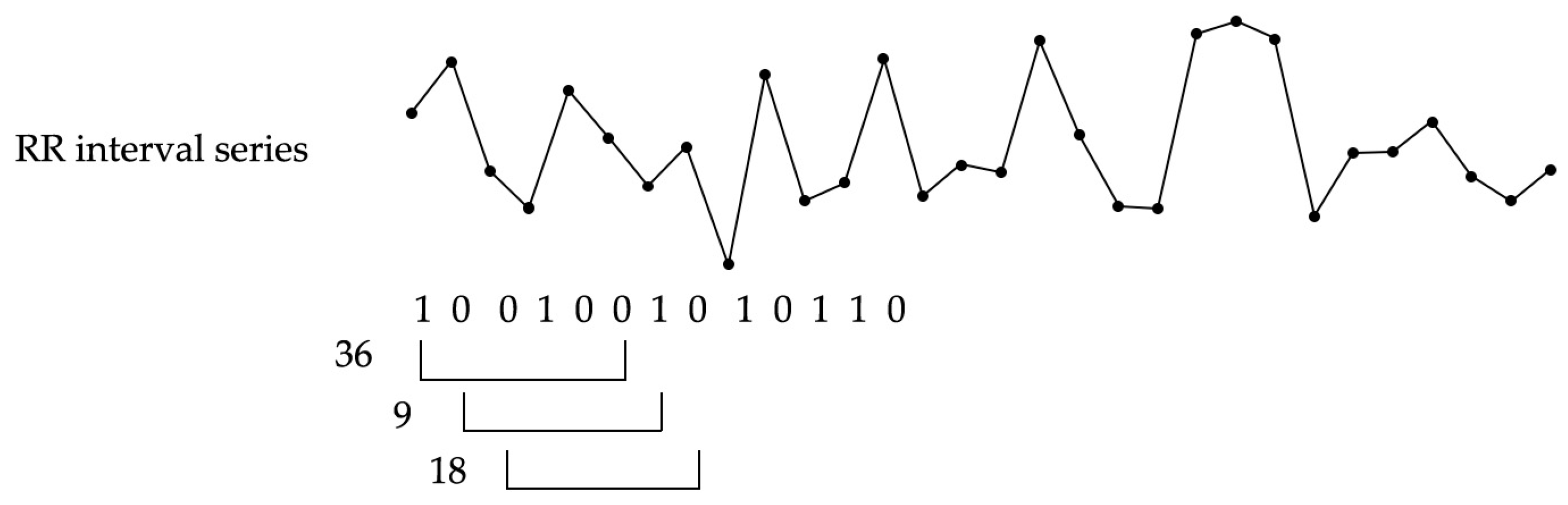
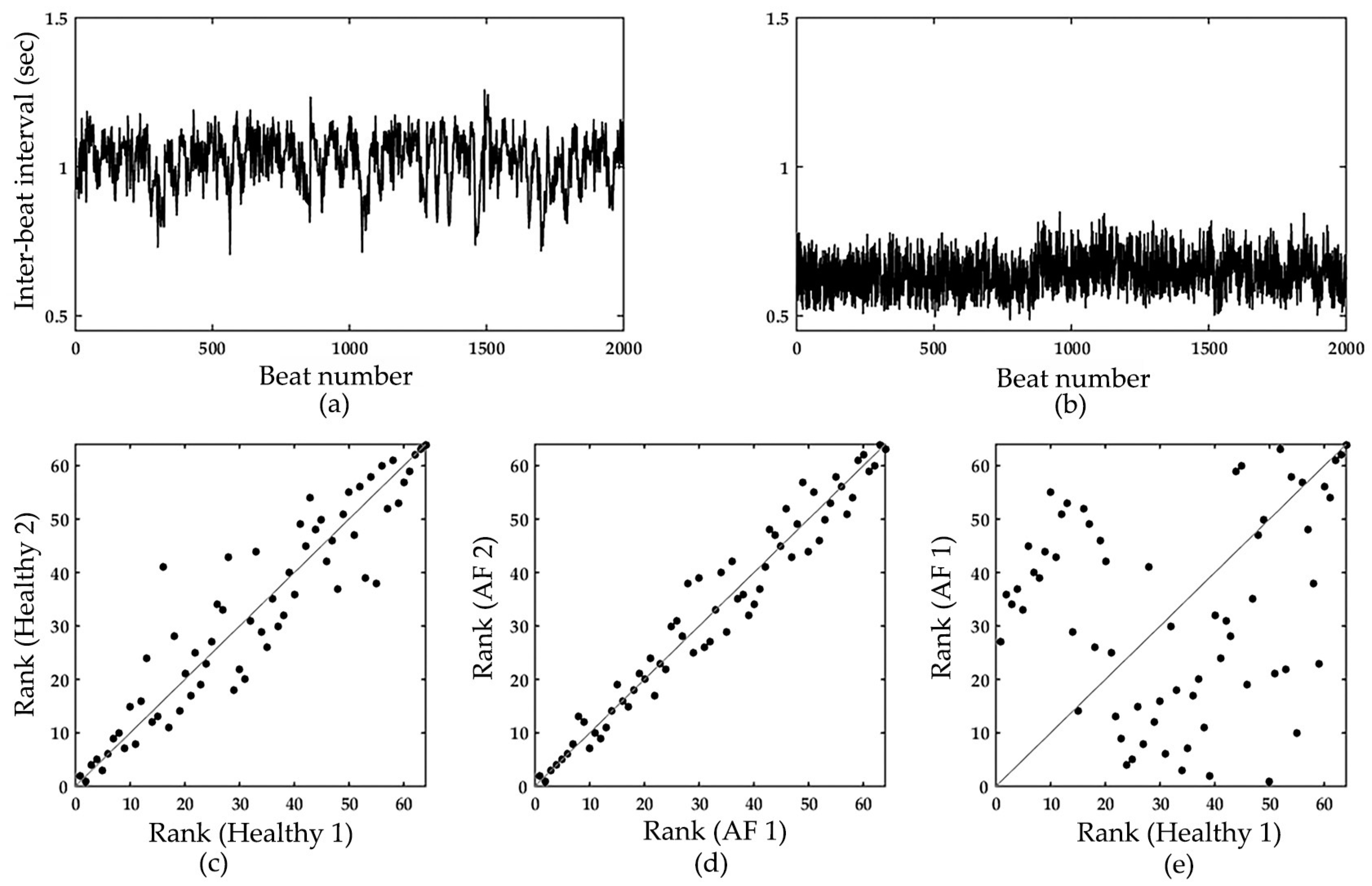
2.2. Information-Based Similarity Index

We have previously proposed an algorithm to measure the distance or dissimilarity between two symbolic sequences [33,34,35,36]. The algorithm is based on measuring differences in the occurrence of repetitive patterns between two symbolic sequences. In this study, the RR-interval time series was mapped to a binary symbolic sequence, where an increase in the RR-interval was represented by ‘1’ and no change or a decrease in the RR-interval was represented by ‘0’. We map m + 1 successive intervals to a binary sequence of length m, called an m-bit “word”. Each m-bit word, therefore, represents a unique pattern of fluctuations in a given RR-interval time series. By shifting one data point at a time, the algorithm produces a collection of m-bit words over the whole time series (total of 2m possible words). Therefore, it is plausible that the occurrence of these m-bit words reflects the underlying dynamics of the original RR time series. Different patterns of dynamics thus produce different distributions of these m-bit words.
Figure 2 illustrates this mapping procedure using 6-bit words (m = 6) from a part of the RR-interval time series. For m = 6, there are a total of 64 (=26) possible words. The first binary word (100100) shown in Figure 2 is equivalent to decimal number of 36 (1 × 25 + 1 × 22 = 36), so as (001001) and (010010) are termed 9 and 18 respectively.
These m-bit words are then sorted according to their frequency of occurrence. The rank-frequency of any given m-bit word may differ between the two sequences mapped from two RR interval time series. We then plot the rank order of each m-bit word in the first symbolic sequence against its rank order in the second symbolic sequence (Figure 3). Each data point on the graph represent a binary word with its rank on first symbolic sequence (horizontal axis) plotted against that on second symbolic sequence on vertical axis. The diagonal line of identity indicates equal rank order for both signal series. If two symbolic sequences are similar in their rank order, the data points will be located near this diagonal line (Figure 3c,d), comparisons between RR time series for either two AF patients or two healthy subjects). The average deviation of the plotted points from the dashed diagonal line is, therefore, a measure of the distance between two symbolic sequences. Greater distance indicates less similarity (Figure 3e, comparison between AF and normal RR time series), and, vice versa.
Let d r ( ψ 1 , ψ 2 ) denote a dissimilarity value between 0 and 1 of two symbolic sequences, s k denote an m-bit word, and L denote the number of unique m-bit words. Let R and p denote the word’s rank and probability, respectively. Let F denote the weight of the word, where F is computed using Shannon’s entropy and normalized with the normalization factor Z. The degree of dissimilarity between two symbolic sequences can be defined as [16,17,18]:
d r ( ψ 1 , ψ 2 ) = 1 L k = 1 L | R 1 ( s k ) R 2 ( s k ) | F ( s k )
F ( s k ) = [ p 1 ( s k ) log p 1 ( s k ) p 2 ( s k ) log p 2 ( s k ) ] / Z
Z = k = 1 L [ p 1 ( s k ) log p 1 ( s k ) p 2 ( s k ) log p 2 ( s k ) ]
The sum is divided by the value L to keep d r ( ψ 1 , ψ 2 ) in the range [0, 1]. A bigger dissimilarity value corresponds to a higher degree of dissimilarity. Therefore, if for an unknown RR-interval series, d N > d A F , where d N is the dissimilarity value between unknown series and normal RR series, and d A F is the dissimilarity value between unknown series and AF RR series, the unknown series is more similar to AF, and vice versa.

2.3. Ensemble Model of Automated AF Detector

2.3.1. Overall Algorithm of the Ensemble Model

The development of this proposed ensemble AF detector follows five key steps:
  • Retrieving sets of AF and NSR RR-interval series from PhysioNet ECG data;
  • randomly setting aside a percentage of AF and NSR sets as training data and the rest as testing data. In AF training data, only AF segments were picked according to annotations provided on the PhysioNet database. This procedure was repeated five times such that five datasets (i.e., datasets 1–5) with different training and testing data could be generated;
  • extracting RR-interval increment signatures (i.e., the rank-frequency of m-bit word) of the desired observation window length from training and testing data, respectively;
  • building templates to represent AF and NSR signature patterns;
  • designing an ensemble classifier, which is composed of various pairs of AF and NSR templates;
  • comparing the information-based dissimilarity index between an unknown RR-interval time series and the templates; and
  • tuning ensemble parameters to achieve our twin aims of high detection accuracy and low detection variance.

2.3.2. Weighted Dissimilarity Index

Since cardiac patterns can be quite variable between different subjects and even within the same subject, the single template approach of averaging multiple and lengthy ECG signals together could result in dilution of significant patterns and data. We thus propose creating multiple AF and NSR templates from shorter observation-window segments and incorporating the ensemble method to obtain better predictive performance for detecting AF. Furthermore, we propose using a weighted variation of bootstrap aggregating (bagging) to perform weighted voting when comparing an unknown RR-interval time series with AF and NSR templates.
In the current study, we randomly generated 10 AF templates and 15 NSR templates in each dataset. More NSR templates were created due to the greater variability of NSR beat patterns between healthy subjects. Each template was created from a set of observation-window segments extracted from the original RR time series of one subject. To assess accuracy, we tested AF RR time series that were not part of the training data. We analyzed these series and compared their diagnoses to the ground truth provided by annotations from the PhysioNet database. Among the 10 AF and 15 NSR templates, all possible template pair combinations were compared against each testing RR-interval time series segment for a total of 150 dissimilarity comparisons. Each pair of dissimilarities was normalized such that d ˜ A F + d ˜ N = 1 . Weighted sums of the dissimilarity values were then calculated for AF and NSR comparisons and averaged to produce a weighted average AF and NSR dissimilarity values, i.e., weighted dissimilarity index:
D N = 1 T i = 1 T d ˜ N ( i )
D A F = 1 T i = 1 T d ˜ A F ( i )
where d ˜ N and d ˜ A F represent the normalized values of d N and d A F , D N and D A F represent the weighted average of d ˜ N and d ˜ A F . T represents the total number of dissimilarity pair comparisons. In this study, T = 150.

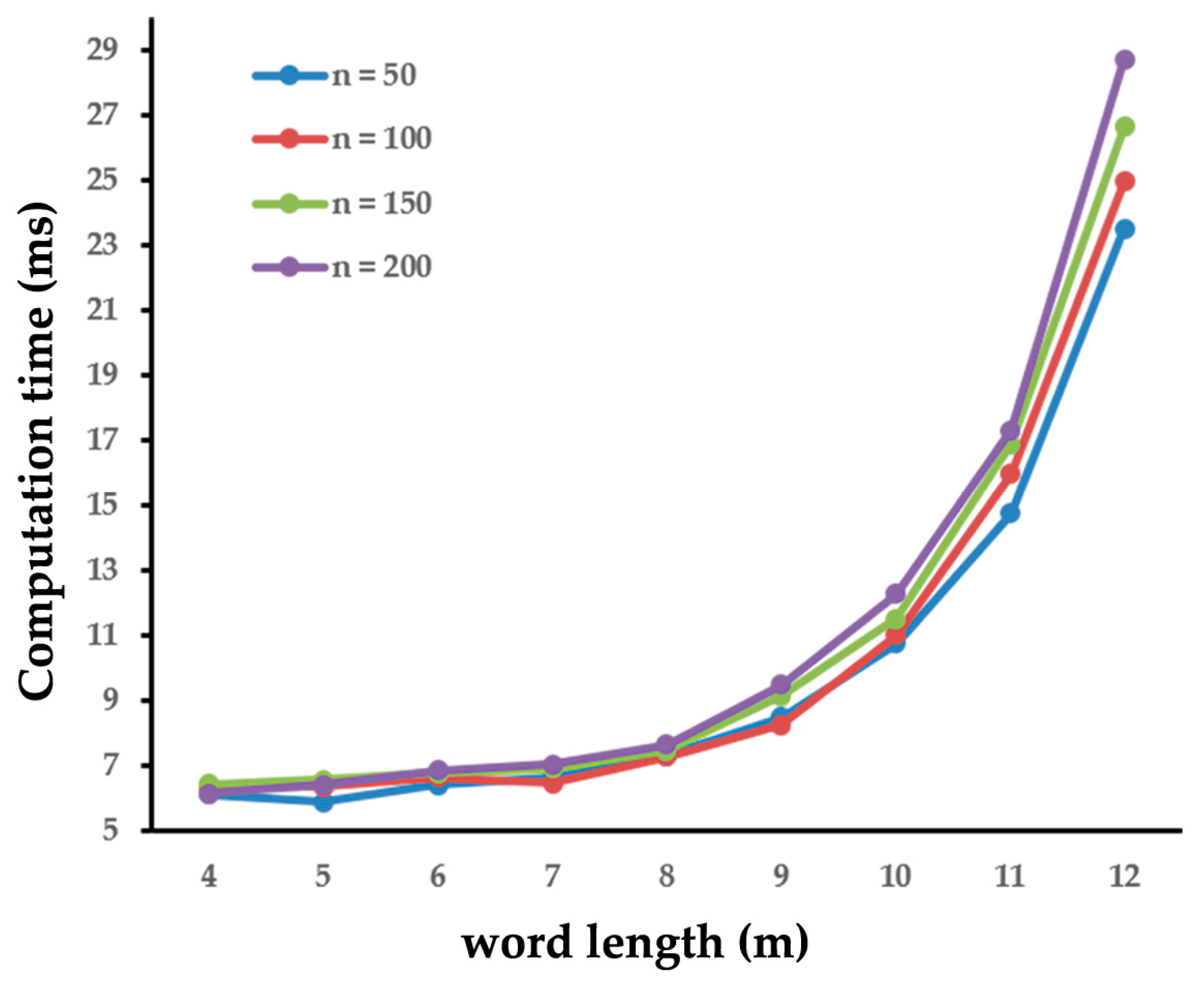
2.3.3. Parameter Tuning

In addition to the m and n parameters, we include a tuning parameter Δ to optimize our final results. The final step in our computation is to compare weighted averages of AF and NSR dissimilarity values, where the smaller dissimilarity index determines the predicted diagnosis of a given test segment. While AF detection accuracy remains high, with optimum accuracies between 98–100%, the NSR accuracy can fall as low as 70% to 80%. When observing the normalized dissimilarity values, many of the false positive diagnoses during NSR testing had very close AF and NSR dissimilarity values that were close to a 50/50 weighting (e.g., a 0.49 weighted AF dissimilarity index compared to a 0.51 NSR weighted dissimilarity index). Although the dissimilarities were close in value, our greater/less than comparison scheme caused many NSR segments to be falsely diagnosed as AF. Using a bias factor to adjust decision boundary is a well-established statistical method when training data may exhibit imbalanced distribution [42]. As a result, we implemented a tuning parameter Δ to shift the dissimilarity comparison boundary and yield more accurate results, where if DN > DAF + Δ, then the segment is AF. Otherwise, the segment is non-AF. For each m-bit word and observation window n combination, we tested Δ values between 0.00 and 0.19 to find the optimum sensitivity and specificity combination.
Thus, in our ensemble model, we use three parameters: the word length m, observation window n, and a bias parameter Δ. We experimented with m from 4 to 12, n from 50 to 200, and Δ of different values. We aimed to find the best parameter setting(s) and sensitivity of different parameter settings. To evaluate the predictive performance of our ensemble model, the sensitivity (SEN), specificity (SPE) and overall accuracy (ACC) were calculated, and repeated cross-validation were performed. SEN is defined as (True Positive)/(True Positive + False Negative), SPE is defined as (True Negative)/(True Negative + False Positive), and ACC is defined as (True Negative + True Positive)/(True Negative + True Positive + False Negative + False Positive).

3. Results

3.1. Overall Performance of the Ensemble Model

Our ensemble model achieved great performance. Table 1 summarizes the results of SEN, SPE and ACC of the prediction models with different cross-validation datasets. Optimal AF-detection parameters are m = 9 and observation window of 150, achieving 97.04% sensitivity, 97.96% specificity, and 97.78% overall accuracy. SEN, SPE, and overall ACC vary little despite changes in word length m, observation window n and cross-validation datasets (see Table 1). The performance of the ensemble model (m = 9, n = 150) at changing the tuning parameter Δ is shown in Table 2. The ensemble model had best performance with Δ = 0.08, achieving 96.30% sensitivity, 98.71% specificity and 98.41% accuracy.

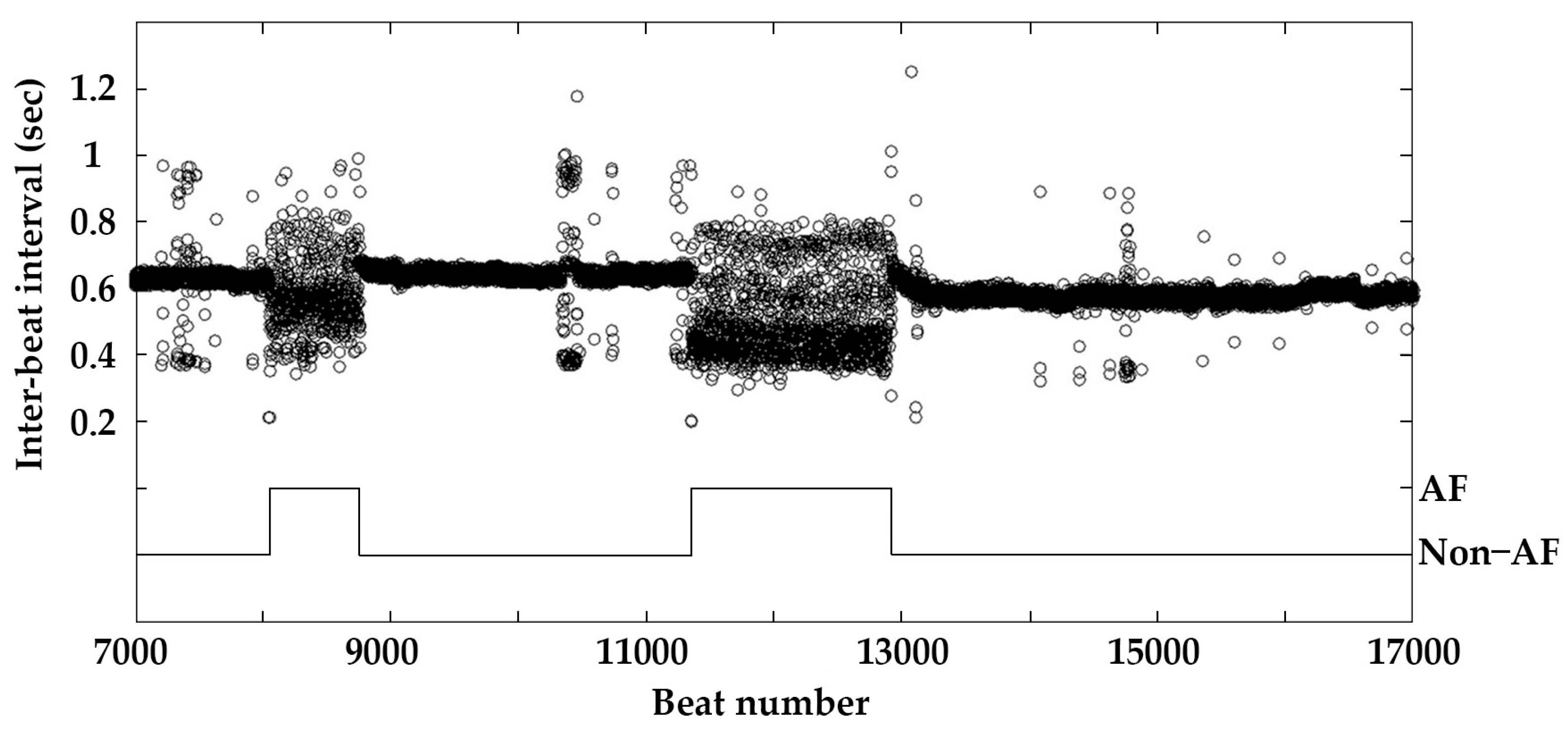
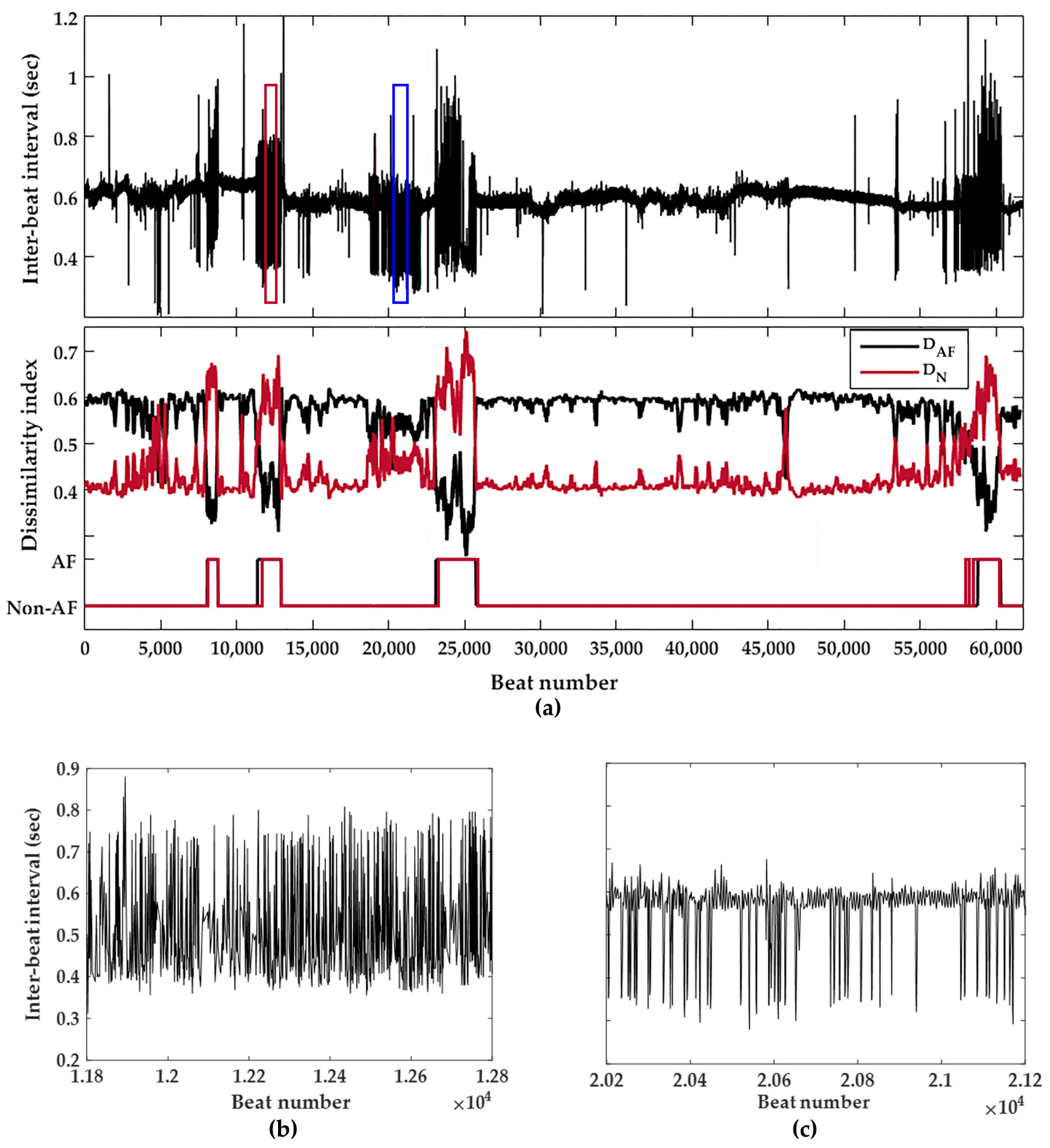
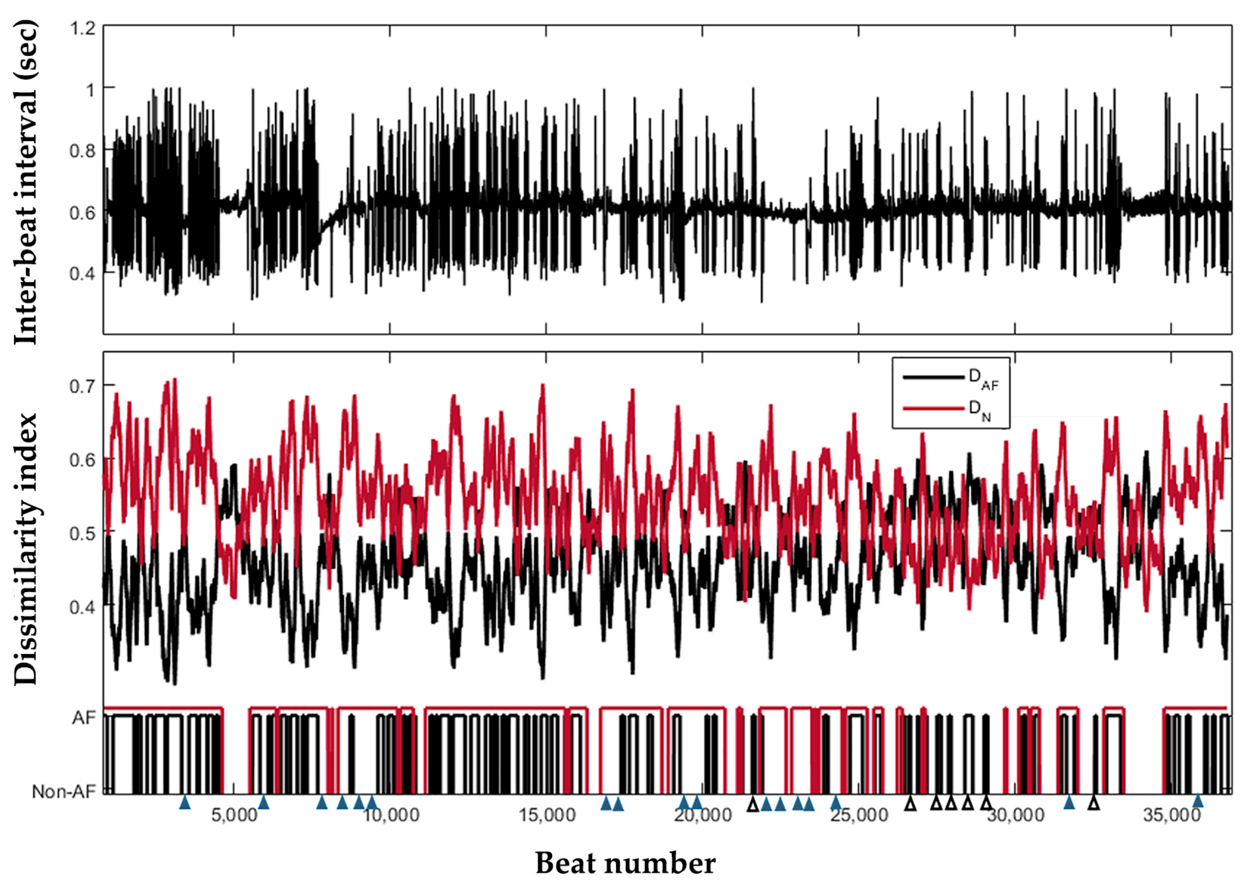
3.2. Continuous Behavior of the Detector

Here we present a graphic description of the testing results using the proposed ensemble detection model for the case of m = 9, the observation window n = 150, and Δ = 0.1 (see Figure 4). The representative testing data in Figure 4 was taken from PhysioNet MIT-BIH AFDB database, record number 04908. The upper panel in Figure 4a displays the testing data, i.e., 10-h raw RR-interval time series recorded from a PAF patient. The lower panel in Figure 4a displays the testing results: D A F (the black curve) represents the weighted average dissimilarity index between testing RR-interval time series and AF templates and D N (the red curve) represents weighted average dissimilarity index between testing RR-interval time series and NSR templates. D A F + 0.1 > D N indicates the dynamic patterns of the testing RR intervals are similar to normal beats, otherwise, the testing RR intervals are similar to AF beats. The black step line indicates the ground truth of the AF episodes (marked as AF or non-AF on y axis) as reported in the annotations of PhysioNet database, and the detection results of testing data are shown in the red step line, achieving 94.40% sensitivity, 99.59% specificity, and 97.01% overall accuracy. Moreover, we enlarge a representative AF segment (see the red rectangle in Figure 4a) to show the detailed fluctuations of AF episode (see Figure 4b). In addition to normal beats, our detection model can successfully distinguish AF episode from non-AF fluctuations, e.g., the segment of beat number 18,800–22,100 in testing RR-interval time series in Figure 4a, which might be caused by R peak detection failure or other problems in this segment. Compared with AF signal, the time series inside of the blue rectangle in Figure 4a was enlarged to show the signal details, see Figure 4c.
In case of sporadic AF episodes of very short duration (e.g., less than 30 s), performance of the proposed detection model is not satisfying. Here we take record 04043 from MIT-BIH AFDB database as representative example (see Figure 5). The testing RR-interval time series are shown in the upper panel. With m = 9, n = 150, and Δ = 0.05, the weighted average dissimilarity index D A F (the black curve) and D N (the red curve) are calculated and shown in the lower panel. D A F + 0.05 > D N indicates the testing RR intervals are similar to normal beats, otherwise, they are similar to AF beats. The black step line indicates the ground truth, and the red step line indicates detection results (AF or non-AF). The detection performance for this record is 89.55% sensitivity, 67.43% specificity and 72.05% accuracy. The solid and hollow triangles marked on the x axis show some examples of false positive and false negative brief segments.

4. Discussion

4.1. Main Findings

In this study, we present a fully automated ensemble model for AF episode detection based on RR-interval time series, applying a novel approach—information-based similarity index and ensemble scheme. By mapping RR time series to binary sequences and comparing the rank-frequency patterns of m-bit word, this study provides quantitative information to enhance the categorization of AF and normal cardiac rhythms. In addition, using a weighted variation of bagging with multiple AF and NSR templates, we can obtain results with low variance and high accuracy. By performing dissimilarity comparisons across multiple templates, we are able to account for RR-interval increment variations between different subjects. Based on our results, optimal AF-detection parameters are symbolic word length m = 9 and observation window n = 150, achieving 97.04% sensitivity, 97.96% specificity, and 97.78% overall accuracy. Sensitivity, specificity, and overall accuracy vary little despite changes in m and n parameters. Our findings indicate that the information-based similarity index is relatively reliable in distinguishing AF episode within considerably long time ECG recordings.

4.2. Advantages of Ensemble Model

AF and NSR patterns may not be consistent among different subjects. In addition, not only do different patients exhibit different patterns, but ECG fluctuates from the same subject throughout different activities, such as during wakefulness versus during sleep. This first observation leads us to design multiple templates for each target class to sufficiently represent AF and NSR patterns. Second, a final class detection, AF or NSR, should be a joint decision made by a committee (or an ensemble), with each member consisting of an AF and NSR template pair. The final decision is made through voting by the committee members. When a committee member strongly endorses one class over the other, that member’s vote should be weighted higher compared to the vote of a “lukewarm” committee member.
This observation motivated us to design a weighted voting scheme, which enforces high confidence votes but discounts low confidence votes. The empirical study shows that such an ensemble scheme reduces detection noise and hence leads to lower detection variance.

4.3. Comparison with Published Works

Many algorithms have been developed to detect AF based in RR interval variability [11,12,13,14,15,16,17,18,19,20,21,22,23,24,25]. Here, we compare the performance of the proposed detector with the existing algorithms published in the last 10 years, which used the same databases (i.e., the same records from MIT-BIH AFDB and the same reference annotations), and using the same evaluation metrics. Table 3 summarizes the comparison results. More complete investigations are available in [21,22,43] The proposed method achieve 97.04% sensitivity, 97.96% specificity, and 97.78% overall accuracy, which is better than most of the previous methods, except the method proposed by Zhou, et al. (97.37% sensitivity, 98.44% specificity, and 97.99% accuracy) [22], and the method proposed by Petrėnas, et al. (97.12% sensitivity and 98.28% specificity) [20].
Most of the detectors in Table 3 employ a window length of 127/128 beats, i.e., [15,16,18,19,21,22], however, detectors with a 128-beat window tend to miss brief clinical episodes. It is important to also consider the ability to detect brief AF episodes when evaluating detector performance. Table 3 also compared the shortest length of the detected AF episodes. The proposed method investigated the performance of the detector from 50 beats to 200 beats. With short detection window n = 50 beats, it achieving 89.58% sensitivity, 90.32% specificity, and 90.04% accuracy (see Table 1). The proposed detection process involves the estimation of probabilities, and a shorter window implies increased statistical uncertainty. Petrėnas, et al. [20], Lee et al. [19], Lake, et al. [23] and Lian et al. [15] reported on performance for shorter windows. Specially, Lake, et al. [23] worked on short window of 12 beats (91% sensitivity and 94% specificity). Petrėnas, et al. [20] used a even shorter window of only 8 beats.
Figure 6 shows the computation time according to word length m and observation window n, with Δ changing from 0.00 to 0.19 in each computation. Compared to the observation window, the word length has more influence to the computation time. The computation time is between 6.09 and 6.42 ms with m = 4, and between 23.51 and 28.72 ms with m = 12. With the optimal AF-detection parameters (m = 9, n = 150), the computation time is 9.12 ms (programs run in MATLAB R2015a on Intel(R) Core(TM) i7-6700k CPU @ 4.00GHz processor, Lenovo, Beijing, China). This shows that our algorithm can be realizable in real time for practical applications, and it is faster than many other algorithms: 20 ~ 30 ms with observation seg = 128, and 3 ~ 4 ms with seg = 12 in Lee et al. [19], 5.2 s with seg = 128 in Lake and Moorman [23], 200 ms with seg = 128 in Dash et al. [18], and 3 s with seg = 100 in Tateno and Glass [12].

4.4. Study Limitations and Future Work

The selection of the observation window places a lower boundary on the length of AF episode that can be detected. This approach is suitable for AF episodes that are prolonged, and the detection results reveal limited performance for sporadic AF episodes of very short duration (e.g., less than 30 s). From a diagnostic point of view, using multiple and complementary methods to detect AF episode may be helpful. Our new approach complements conventional approaches of AF detection, since our algorithm is based on a completely different concept from other approaches. This algorithm may also be easily adapted to other physiological and physical time series data, provided that a meaningful symbolic mapping rule can be defined.
We propose the implementation of a confidence-based voting scheme due to the disproportionate weighting that may be given to certain dissimilarity values. For example, if a dissimilarity computation for a given test segment in one case yields a 0.90 AF dissimilarity and a 0.95 NSR dissimilarity, the values suggest that the test segment is quite dissimilar from both templates. However, normalization of the dissimilarity values results in a normalized value of 0.47 AF dissimilarity and 0.53 NSR dissimilarity. In a second case where a test segment yields a 0.15 AF dissimilarity and a 0.10 NSR dissimilarity, the test segment is much more similar to each segment and thus its weighting may be more significant. However, the dissimilarity values would be normalized to approximately 0.60 AF and 0.40 NSR, which are not too different from that of the first case. In a future study, we aim to test whether dissimilarity values such as those in the first case should be regarded with less confidence than dissimilarity values of the second case.
In addition to confidence-based voting, to further improve and validate our results, we will also perform cross validation with different sets of training data from the AFDB and NSRDB to validate our current results.

Acknowledgments

This study was supported by “the Fundamental Research Funds for the Central Universities” of China (Grant No. 3207037101), and the Delta Environmental & Educational Foundation.

Author Contributions

Xingran Cui, Chung-Kang Peng and Albert C. Yang conceived and designed the study; Wen-Hung Yang and Bernard C. Jiang performed the experiments; Xingran Cui, Wen-Hung Yang, Emily Chang analyzed the data; Xingran Cui wrote the paper. All authors were involved with the editing of the publication, approval of the data, reported findings, and final version of the publication.

Conflicts of Interest

The authors declare no conflict of interest.

References

  1. Iwasaki, Y.-K.; Nishida, K.; Kato, T.; Nattel, S. Atrial Fibrillation Pathophysiology. Circulation 2011, 124, 2264–2274. [Google Scholar] [CrossRef] [PubMed]
  2. Munger, T.M.; Wu, L.Q.; Shen, W.K. Atrial fibrillation. J. Biomed. Res. 2014, 28, 1–17. [Google Scholar] [PubMed]
  3. January, C.T.; Wann, L.S.; Alpert, J.S.; Calkins, H.; Cigarroa, J.E.; Cleveland, J.C., Jr.; Conti, J.B.; Ellinor, P.T.; Ezekowitz, M.D.; Field, M.E.; et al. 2014 AHA/ACC/HRS guideline for the management of patients with atrial fibrillation: A report of the American College of Cardiology/American Heart Association Task Force on Practice Guidelines and the Heart Rhythm Society. J. Am. Coll. Cardiol. 2014, 64. [Google Scholar] [CrossRef]
  4. Israel, C.W.; Grönefeld, G.; Ehrlich, J.R.; Li, Y.G.; Hohnloser, S.H. Long-term risk of recurrent atrial fibrillation as documented by an implantable monitoring device: Implications for optimal patient care. J. Am. Coll. Cardiol. 2004, 43, 47–52. [Google Scholar] [CrossRef] [PubMed]
  5. Page, R.L.; Wilkinson, W.E.; Clair, W.K.; McCarthy, E.A.; Pritchett, E.L. Asymptomatic arrhythmias in patients with symptomatic paroxysmal atrial fibrillation and paroxysmal supraventricular tachycardia. Circulation 1994, 89, 224–227. [Google Scholar] [CrossRef] [PubMed]
  6. Andresen, D.; Bruggemann, T. Heart rate variability preceding onset of atrial fibrillation. J. Cardiovasc. Electrophysiol. 1998, 9, S26–S29. [Google Scholar] [PubMed]
  7. Glass, L.; Tateno, K. A method for detection of atrial fibrillation using the RR intervals. Comput. Cardiol. 2000, 27, 391–394. [Google Scholar]
  8. Langley, P.; Bourke, J.P.; Murray, A. Frequency analysis of atrial fibrillation. Comput. Cardiol. 2000, 27, 65–68. [Google Scholar]
  9. Stridh, M.; Sornmo, L. Spatiotemporal QRST cancellation techniques for analysis of atrial fibrillation. IEEE Trans. Biomed. Eng. 2001, 48, 105–111. [Google Scholar] [CrossRef] [PubMed]
  10. Fischer, R.; Klein, G.; Widiger, B.; Hoy, L.; Zywietz, C. Discrimination between atrial flutter and atrial fibrillation by computing a flutter index. Comput. Cardiol. 2005, 32, 81–84. [Google Scholar]
  11. Moody, G.; Mark, R. A new method for detecting atrial fibrillation using R-R intervals. Comput. Cardiol. 1983, 10, 227–230. [Google Scholar]
  12. Tateno, K.; Glass, L. Automatic detection of atrial fibrillation using the coefficient of variation and density histograms of RR and deltaRR intervals. Med. Biol. Eng. Comput. 2001, 39, 664–671. [Google Scholar] [CrossRef] [PubMed]
  13. Kikillus, N.; Hammer, G.; Lentz, N.; Stockwald, F.; Bolz, A. Three different algorithms for identifying patients suffering from atrial fibrillation during atrial fibrillation free phases of the ECG. In Proceedings of the Computers in Cardiology, Durham, NC, USA, 30 September–3 October 2007; Volume 34, pp. 801–804. [Google Scholar]
  14. Babaeizadeh, S.; Gregg, R.E.; Helfenbein, E.D.; Lindauer, J.M.; Zhou, S.H. Improvements in atrial fibrillation detection for real-time monitoring. J. Electrocardiol. 2009, 42, 522–526. [Google Scholar] [CrossRef] [PubMed]
  15. Lian, J.; Wang, L.; Muessig, D. A simple method to detect atrial fibrillation using RR intervals. Am. J. Cardiol. 2011, 107, 1494–1497. [Google Scholar] [CrossRef] [PubMed]
  16. Huang, C.; Ye, S.; Chen, H.; Li, D.; He, F.; Tu, Y. A novel method for detection of the transition between atrial fibrillation and sinus rhythm. IEEE Trans. Biomed. Eng. 2011, 58, 1113–1119. [Google Scholar] [CrossRef] [PubMed]
  17. Parvaresh, S.; Ayatollahi, A. Automatic atrial fibrillation detection using autoregressive modeling. In Proceedings of the 2011 International Conference on Biomedical Engineering and Technology, Kuala Lumpur, Malaysia, 4–5 June 2011; pp. 105–108. [Google Scholar]
  18. Dash, S.; Chon, K.; Lu, S.; Raeder, E. Automatic real time detection of atrial fibrillation. Ann. Biomed. Eng. 2009, 37, 1701–1709. [Google Scholar] [CrossRef] [PubMed]
  19. Lee, J.; Nam, Y.; McManus, D.D.; Chon, K.H. Time-Varying Coherence Function for Atrial Fibrillation Detection. IEEE Trans. Biomed. Eng. 2013, 60, 2783–2793. [Google Scholar] [PubMed]
  20. Petrenase, A.; Marozas, V.; Sönmo, L. Low-complexity detection of atrial fibrillation in continuous long term monitoring. Comput. Biol. Med. 2015, 60, 2783–2793. [Google Scholar] [CrossRef] [PubMed]
  21. Zhou, X.; Ding, H.; Ung, B.; Pickwell-MacPherson, E.; Zhang, Y. Automatic Online Detection of Atrial Fibrillation Based on Symbolic Dynamics and Shannon Entropy. Biomed. Eng. Online 2014, 13, 1–18. [Google Scholar] [CrossRef] [PubMed]
  22. Zhou, X.; Ding, H.; Wu, W.; Zhang, Y. A Real-Time Atrial Fibrillation Detection Algorithm Based on the Instantaneous State of Heart Rate. PLoS ONE 2015, 10, e0136544. [Google Scholar] [CrossRef] [PubMed]
  23. Lake, D.; Moorman, J. Accurate estimation of entropy in very short physiological time series: The problem of atrial fibrillation detection in implanted ventricular devices. Am. J. Physiol. Heart Circ. Physiol. 2011, 300, H319–H325. [Google Scholar] [CrossRef] [PubMed]
  24. Carrara, M.; Carozzi, L.; Moss, T.J.; de Pasquale, M.; Cerutti, S.; Lake, D.E.; Moorman, J.R.; Ferrario, M. Classification of cardiac rhythm using heart rate dynamical measures: Validation in MIT-BIH databases. J. Electrocardiol. 2015, 48, 943–946. [Google Scholar] [CrossRef] [PubMed]
  25. Carrara, M.; Carozzi, L.; Moss, T.J.; de Pasquale, M.; Cerutti, S.; Ferrario, M.; Lake, D.E.; Moorman, J.R. Heart rate dynamics distinguish among atrial fibrillation, normal sinus rhythm and sinus rhythm with frequent ectopy. Physiol. Meas. 2015, 36, 1873–1888. [Google Scholar] [CrossRef] [PubMed]
  26. Masè, M.; Disertori, M.; Marini, M.; Ravelli, F. Characterization of rate and regularity of ventricular response during atrial tachyarrhythmias. Insight on atrial and nodal determinants. Physiol. Meas. 2017, 38, 800–818. [Google Scholar] [CrossRef] [PubMed]
  27. Lian, J.; Mussig, D.; Lang, V. Computer modeling of ventricular rhythm during atrial fibrillation and ventricular pacing. IEEE Trans. Biomed. Eng. 2006, 53, 1512–1520. [Google Scholar] [CrossRef] [PubMed]
  28. Lerma, C.; Trine, K.M.; Guevara, M.; Glass, L. Stochastic aspects of cardiac arrhythmias. J. Stat. Phys. 2007, 128, 347–374. [Google Scholar] [CrossRef]
  29. Zeng, W.; Glass, L. Statistical properties of heartbeat intervals during atrial fibrillation. Phys. Rev. E Stat. Phys. Plasmas Fluids Relat. Interdiscip. Top. 1996, 54, 1779–1784. [Google Scholar] [CrossRef]
  30. Costa, M.; Goldberger, A.L.; Peng, C.-K. Multiscale entropy analysis of complex physiologic time series. Phys. Rev. Lett. 2002, 89, 068102. [Google Scholar] [CrossRef] [PubMed]
  31. Costa, M.; Goldberger, A.L.; Peng, C.-K. Multiscale entropy analysis of biological signals. Phys. Rev. E 2005, 71. [Google Scholar] [CrossRef] [PubMed]
  32. Peng, C.-K.; Costa, M.; Goldberger, A.L. Adaptive data analysis of complex fluctuations in physiologic time series. Adv. Adapt. Data Anal. 2009, 1, 61–70. [Google Scholar] [CrossRef] [PubMed]
  33. Yang, A.C.; Hseu, S.S.; Yien, H.W.; Goldberger, A.L.; Peng, C.K. Linguistic analysis of the human heartbeat using frequency and rank order statistics. Phys. Rev. Lett. 2003, 90, 108103. [Google Scholar] [CrossRef] [PubMed]
  34. Yang, A.C.; Goldberger, A.L.; Peng, C.K. Genomic classification using an information-based similarity index: application to the SARS coronavirus. J. Comput. Biol. 2005, 12, 1103–1116. [Google Scholar] [PubMed]
  35. Yang, A.C.; Peng, C.K.; Yien, H.W.; Goldberger, A.L. Information categorization approach to literary authorship disputes. Phys. A Stat. Mech. Appl. 2003, 329, 473–483. [Google Scholar] [CrossRef]
  36. Peng, C.K.; Yang, A.C.C.; Goldberger, A.L. Statistical physics approach to categorize biologic signals: From heart rate dynamics to DNA sequences. Chaos 2007, 17, 015115. [Google Scholar] [CrossRef] [PubMed]
  37. Christini, D.J.; Glass, L. Introduction: Mapping and control of complex cardiac arrhythmias. Chaos 2002, 12, 732–739. [Google Scholar] [CrossRef] [PubMed]
  38. Hall, K.; Christini, D.J.; Tremblay, M.; Collins, J.J.; Glass, L.; Billette, J. Dynamic control of cardiac alternans. Phys. Rev. Lett. 1997, 78, 4518–4521. [Google Scholar] [CrossRef]
  39. Goldberger, A.L.; Amaral, L.A.; Glass, L.; Hausdorff, J.M.; Ivanov, P.C.; Mark, R.G.; Mietus, J.E.; Moody, G.B.; Peng, C.-K.; Stanley, H.E. PhysioBank, PhysioToolkit, and PhysioNet: Components of a new research resource for complex physiologic signals. Circulation 2000, 101, E215–E220. [Google Scholar] [CrossRef] [PubMed]
  40. Moody, G.B.; Mark, R.G.; Goldberger, A.L. PhysioNet: A research resource for studies of complex physiologic and biomedical signals. Comput. Cardiol. 2000, 27, 179–182. [Google Scholar] [PubMed]
  41. Costa, M.; Moody, G.B.; Henry, I.; Goldberger, A.L. PhysioNet: An NIH research resource for complex signals. J. Electrocardiol. 2003, 36, 139–144. [Google Scholar] [CrossRef] [PubMed]
  42. Wu, G.; Chang, E.Y. KBA: Kernel Boundary Alignment Considering Imbalanced Data Distribution. IEEE Trans. Knowl. Data Eng. 2005, 17, P786–P795. [Google Scholar] [CrossRef]
  43. Larburu, N.; Lopetegi, T.; Romero, I. Comparative study of algorithms for Atrial Fibrillation detection. In Proceedings of the Conference on Computing in Cardiology, Hangzhou China, 18–21 September 2011; Volume 38, pp. 265–268. [Google Scholar]
  44. Couceiro, R.; Carvalho, P.; Henriques, J.; Antunes, M.; Harris, M.; Habetha, J. Detection of atrial fibrillation using model-based ECG analysis. In Proceedings of the 19th International Conference on Pattern Recognition, Tampa, FL, USA, 8–11 December 2008; pp. 1–5. [Google Scholar]
Figure 1. Representative inter-beat (RR) interval time series derived from an electrocardiographic recording of a patient with paroxysmal atrial fibrillation. The dark circles represent consecutive RR intervals and the solid line indicates the presence/absence of AF episodes as reported in the annotations of PhysioNet database. During an episode of atrial fibrillation, the line is set to “AF”; otherwise it is set to “Non-AF”, which means a rhythm that is not atrial fibrillation.
Entropy 19 00677 g001
Figure 2. Schematic illustration of the mapping procedure for 6-bit words (m = 6).
Entropy 19 00677 g002
Figure 3. Representative inter-beat time series for a healthy subject (a) and an AF patient (b); (c) Rank order comparison of the time series for two healthy subjects; (d) Rank order comparison of the time series for two AF patients; (e) Rank order comparison of the time series in (a,b). The results in (ce) are for the case m = 6.
Entropy 19 00677 g003
Figure 4. (a) Graphic illustration of detection results for a testing data (record 04908, m = 9, observation window n = 150, Δ = 0.1); (b) enlarged AF segment derived from (a); (c) Enlarged signal segment of neither AF nor normal beats to compare with (b).
Entropy 19 00677 g004
Figure 5. Graphic illustration of detection results for a testing data (record 04043, m = 9, n = 150, Δ = 0.05).
Entropy 19 00677 g005
Figure 6. Computation time according to m and n (the computation times are the average values of 100 trials).
Entropy 19 00677 g006
Table 1. Detection performances (%) of changing m and n parameters.
mRepeated Cross-ValidationObservation Window Size (n)
50100150200
SENSPEACCSENSPEACCSENSPEACCSENSPEACC
4Dataset 186.3486.4686.4493.0693.4993.4394.7494.1494.2196.6296.2896.32
Dataset 285.7187.0986.1591.1792.0091.6694.1293.6393.9095.0295.1195.08
Dataset 383.6086.0885.5990.6189.0589.9995.2896.0295.7190.3392.5091.87
Dataset 486.4986.0386.5592.6793.0292.8093.0693.2293.1992.4993.4493.06
Dataset 585.0984.6684.8691.9390.9591.2595.1996.7996.2093.8895.3894.91
Average85.4586.0685.9291.8991.7091.8394.4894.7694.6493.6794.5494.25
5Dataset 186.3485.1585.3493.0693.0693.0695.3294.7394.8196.6295.9296.01
Dataset 286.4587.8587.0989.8590.7090.1194.4994.0594.2091.3892.1292.03
Dataset 387.5786.5486.9792.3393.3792.9095.0296.1295.8695.7795.2695.50
Dataset 485.2384.8385.0192.2892.5592.4493.6694.5294.2096.1394.9495.36
Dataset 588.0088.5288.4393.5092.7193.2594.4794.7194.5595.3295.8895.72
Average86.7286.5886.5792.2092.4892.3594.5994.8394.7295.0494.8294.92
6Dataset 187.3988.1188.0093.2793.3193.3096.4995.1695.3296.1496.9996.88
Dataset 287.3386.4086.9495.4496.0495.8194.8195.2995.1594.6595.0894.89
Dataset 390.8891.9891.6094.1894.0594.0796.0696.5796.4496.7796.5196.60
Dataset 486.4785.9086.0791.4692.6992.5095.9096.4796.3995.0296.3396.19
Dataset 587.8987.6687.7291.0792.3392.2696.3295.9096.0294.9495.3895.26
Average87.9988.0188.0793.0893.6893.5995.9295.8895.8695.5096.0695.96
7Dataset 189.5989.4789.4994.6994.0394.1396.7895.6595.7997.1097.0697.07
Dataset 288.0487.2387.4091.5692.8692.4296.1396.6096.4194.4493.9594.10
Dataset 390.1491.2990.2595.2295.7095.5897.4698.3998.1895.4595.0295.13
Dataset 487.3787.0587.1094.3194.5794.5195.0895.2395.1795.4895.6695.62
Dataset 590.5190.2690.2993.0692.9192.9697.5898.4198.3394.8796.8196.67
Average89.1388.8688.9193.7794.0193.9296.6196.8696.7895.4795.7095.72
8Dataset 190.5489.6989.8395.5195.3695.3897.0897.1097.0897.1097.9297.82
Dataset 289.6489.2289.3095.0895.2795.2295.2099.0497.2797.1598.5898.40
Dataset 389.0190.8590.2496.4996.4496.4596.3797.1197.6695.4895.7095.61
Dataset 488.4690.8090.0395.6896.0295.9796.6898.0097.3895.2096.4996.33
Dataset 590.2591.0290.7996.9196.7796.8095.5196.7896.4296.6897.0096.92
Average89.5890.3290.0495.9395.9795.9696.1797.6197.1696.3297.1497.02
9Dataset 190.3589.289.3895.7195.1895.2698.2597.9698.0197.5897.8597.82
Dataset 292.0988.2589.0697.4797.1897.0197.3697.7997.7093.9295.0694.77
Dataset 389.5390.8790.3594.7297.0996.3996.3098.7198.4193.9997.0296.68
Dataset 487.6089.3389.0294.7698.1097.0696.9597.2897.1195.0596.4496.11
Dataset 586.4485.9886.6094.6596.2895.7996.3398.0597.6697.5997.9997.83
Average89.2088.7388.8895.4696.7796.3097.0497.9697.7895.6396.8796.64
10Dataset 189.1189.7389.6396.3395.1195.2997.9596.7796.9497.5897.9997.94
Dataset 289.4590.9290.8495.7395.8895.8494.6995.6695.2895.9597.9396.64
Dataset 388.1587.3288.0395.3394.2595.0296.2698.3197.8195.6492.5593.13
Dataset 485.0687.2886.3796.8596.2096.4696.6497.5397.1997.2695.0595.81
Dataset 586.4085.9186.3997.0198.3398.1796.9598.0397.7295.2896.3395.65
Average87.2787.8687.9196.2595.9596.1696.1497.3897.0096.0395.4795.31
11Dataset 188.7888.4588.6695.5194.7594.8697.6697.5397.5597.5897.7897.88
Dataset 284.5483.9784.1293.7793.9293.8997.8097.1297.2595.5596.7896.42
Dataset 385.3784.9084.7895.7694.8895.0598.1297.5797.6895.9295.4095.51
Dataset 487.7787.9387.8795.1594.7994.9098.0497.6097.8197.9997.2997.45
Dataset 589.7689.4589.5295.3095.9695.8895.8895.2695.3496.6495.9096.07
Average87.2486.9486.9995.1094.8694.9297.5097.0297.1396.7496.6396.67
12Dataset 187.9385.7886.6193.6794.5794.4496.7897.0496.9997.1096.9296.94
Dataset 286.1086.8286.6796.3695.3395.4595.4596.2396.0697.1397.6497.55
Dataset 384.1285.3785.0495.6695.0695.2195.9195.7795.8195.4895.3595.40
Dataset 484.8783.5283.6692.5093.0292.9196.8695.9896.3095.5296.0696.13
Dataset 585.0987.7087.2293.4894.3694.1597.1997.0797.1095.0496.1795.93
Average85.6285.8485.8494.3394.4794.4396.4496.4296.4596.0596.4396.39
Table 2. Performance of the ensemble model (m= 9, n= 150) at changing the tuning parameter Δ.
Tuning Parameter ΔDetection Performance (%)
SENSPEACC
0.0099.5196.3496.73
0.0199.3596.6797.00
0.0299.1997.0497.31
0.0398.7297.3697.53
0.0498.3297.7497.81
0.0597.7798.0598.02
0.0697.3198.2498.13
0.0796.8698.5998.38
0.0896.3098.7198.41
0.0995.4098.7698.34
0.1094.1198.8098.22
0.1192.9998.8498.12
0.1291.6098.8897.98
0.1390.3998.9297.86
0.1489.1098.9697.73
0.1587.8799.0597.66
0.1686.5499.2497.67
0.1783.0399.5997.54
0.1876.7599.7196.86
0.1970.9099.7696.18
Table 3. Comparison of detector performance on the MIT-BIH Atrial Fibrillation Database (AFDB).
MethodYearDatabaseLength of Detected Episodes (Beats)Best Performance (%)
ShortestBestSENSPEACC
Proposed method2017AFDB5015097.0497.9697.78
Zhou, et al. [22]2015AFDB12712797.3798.4497.99
Petrėnas, et al. [20]2015AFDB86097.1298.28-
Zhou, et al. [21]2014AFDB12712796.8998.2597.67
Lee, et al. [19]2013AFDB *1212898.2297.6797.91
Huang, et al. [16]2011AFDB12812896.198.1-
Lake, et al. [23]2011AFDB12129194-
Lian, et al. [15]2011AFDB3212895.995.4-
Parvaresh, et al. [17]2011AFDB *15 s15 s96.1493.20-
Dash, et al. [18]2009AFDB **12812894.495.1-
Babaeizadeh, et al. [14]2009AFDB *--92--
Couceiro, et al. [44]2008AFDB *1210093.896.09-
* Records “00735” and “03665” omitted; ** Records “04936” and “05091” omitted.

