Article

A General Symbolic Approach to Kolmogorov-Sinai Entropy

Institute of Mathematics, University of Lübeck, Ratzeburger Allee 160, 23562 Lübeck, Germany
*
Author to whom correspondence should be addressed.
Entropy 2017, 19(12), 675; https://doi.org/10.3390/e19120675
Submission received: 31 October 2017 / Revised: 4 December 2017 / Accepted: 5 December 2017 / Published: 9 December 2017
(This article belongs to the Special Issue Symbolic Entropy Analysis and Its Applications)

Abstract

:
It is popular to study a time-dependent nonlinear system by encoding outcomes of measurements into sequences of symbols following certain symbolization schemes. Mostly, symbolizations by threshold crossings or variants of it are applied, but also, the relatively new symbolic approach, which goes back to innovative works of Bandt and Pompe—ordinal symbolic dynamics—plays an increasing role. In this paper, we discuss both approaches novelly in one breath with respect to the theoretical determination of the Kolmogorov-Sinai entropy (KS entropy). For this purpose, we propose and investigate a unifying approach to formalize symbolizations. By doing so, we can emphasize the main advantage of the ordinal approach if no symbolization scheme can be found that characterizes KS entropy directly: the ordinal approach, as well as generalizations of it provide, under very natural conditions, a direct route to KS entropy by default.

1. Introduction

Using symbolizations to study observed data plays an important role in today’s time series analysis (see for instance the review papers of Daw et al. [1], Zanin et al. [2], Amigó et al. [3], and the examples in biology, medicine, artificial intelligence and data mining, just to mention a few, given therein). Thereby, it is assumed that time series, given by measurements of a real-world time-dependent system, store information about the complexity of the underlying system, which can be accessed by symbolic dynamics. In this paper, we assume further that measurements provide n-dimensional real-valued outcomes, that is a measuring process provides n time series.
Knowing the complexity is a key to classify systems and to predict future developments. A data analyst can for instance quantify complexity by empirical entropy measures, in particular by estimating the well-defined Kolmogorov-Sinai entropy (KS entropy). In order to estimate the KS entropy, however, a data analyst is always faced with the problem of choosing an adequate symbolization scheme.
Symbolizing a time series could be done in a “classical” manner for example by subdividing the data range into a finite number of intervals (see Section 2.1, often called the threshold crossing method in symbolic dynamics) or in an ordinal manner for example by considering the up and down behavior of subsequent measured values (see Section 2.2). The most ideal, however unrealistic, case is given if the analyst knows the underlying dynamics and picks a generating (under the dynamics) partition (see Section 1.1 and Section 1.4 for the mathematical formulation of the general problem, as well as for instance Crutchfield and Packard [4], Bollt et al. [5] and Kennel and Buhl [6]).
In the present paper, we show, by proposing a unifying approach to formalize symbolizations, that under relatively week assumptions, the search for a generating partition can be skipped if one chooses a symbolization scheme that regards a dependency between two measured values (see Section 2.2). In fact, following some rules by picking such a symbolization scheme, a generating sequence of finite partitions (see Section 1.1 and Section 1.4) is provided by default and needs no further attention (see Section 2.3 for an overview and Section 3 and Section 4.1, as well as the Appendix for the mathematics behind this). Moreover, the unifying approach allows one to consider “classical” and the relatively new ordinal symbolic dynamics [3] hand in hand and therefore to study respective assets and drawbacks.
In terms of the analyst, we propose a supplementing pool of complexity measures, which are in a certain sense approximations of the KS entropy and may be worth being compared in the finite setting of application (see Figure 7). Moreover, the relatively new ordinal approach could benefit from results achieved in “classical” symbolic dynamics, for instance to estimate a good symbolization scheme (see our ending remarks of the paper in Section 5 and for instance Steuer et al. [7], Letellier [8] and, published most recently, Li and Ray [9], as well as the references given therein). However, such topics exceed the scope of this paper.

1.1. Mathematical Formulation of the General Problem

Let us describe the central problems of determining KS entropy and give the main concepts of the paper without going into too much detail. The mathematical formulation is necessary at this point in order to state the results of the paper adequately.
We model a real-world time-dependent system by a state space Ω , that is states ω of the system are taken from the set Ω and events on the system from a σ -algebra A on Ω . We assume that the states are distributed according to a probability distribution μ on ( Ω , A ) . Moreover, considering states of the system at times in N 0 = { 0 , 1 , 2 , } , the dynamics of the system is described by a map T with the interpretation that the system is in state T ( ω ) at time t + 1 if it is in state ω at time t. For mathematical correctness, T is required to be measurable with respect to A . We assume that the distribution of the states does not change in time, meaning T is μ -invariant, which is defined by T 1 ( A ) A for all sets A A .
The KS entropy is based on entropy rates of finite partitions of the state space. Given a finite partition C = C ( 1 ) , C ( 2 ) , , C ( q ) A of Ω , the entropy rate h μ ( T , C ) , roughly speaking, measures the complexity of possible symbolic paths (see Section 4.1). A symbolic path is given by assigning to each state of the orbit:
ω , T ( ω ) , T 2 ( ω ) , T 3 ( ω ) ,
a symbol a when the state is contained in C ( a ) . Here, T t ( ω ) denotes the t-th iterate of ω under T. We emphasize that starting with a partition C = C ( 1 ) , C ( 2 ) , , C ( q ) is equivalent to a start where to each state in Ω a symbol in { 1 , 2 , , q } is assigned (in a measurable way). That is why we use the term symbolic approach.
In order to obtain a complexity measure that is independent of the discretization determined by a finite partition, one takes the supremum of the entropy rate h μ ( T , C ) over all finite partitions C A of Ω , that is the KS entropy h μ KS ( T ) of T:
h μ KS ( T ) : = sup C   finite   partition h μ ( T , C ) .
Since usually there are uncountably many finite partitions, the determination of KS entropy on the basis of the definition is not feasible, so one is interested in finding natural partitions “carrying” the KS entropy.
In the case of a generating partition C under T (see Section 4.1), KS entropy is already characterized by this partition, meaning that:
h μ KS ( T ) = h μ ( T , C )
(see, e.g., Walters [10], Theorem 4.18). Finding such suitable partitions, however, is impossible in most cases. A more realistic way of approaching KS entropy is to look for a generating and increasing, i.e., refining (see Section 4.1), sequence ( C d ) d N of finite partitions C d A of Ω , where:
h μ KS ( T ) = lim d h μ ( T , C d ) = sup d N h μ ( T , C d )
(see, e.g., Walters [10], Theorem 4.22).
In the present paper, we discuss this countable increasing route to KS entropy in a framework where all partitions considered are derived from a natural real-valued “measuring process” and a symbolization scheme determined by a finite partition of the two-dimensional Euclidean space. The discussion includes and generalizes ideas from “classical” symbolic dynamics and from ordinal symbolic dynamics related to permutation entropy and sheds some new light on the latter one.

1.2. Observables and the Measuring Process

The modeling is completed by assuming that an n-dimensional outcome (here, n N = { 1 , 2 , 3 , } ) of the system for each time is provided by observables X 1 , X 2 , , X n , which mathematically are random variables on the probability space ( Ω , A , μ ) with values in the real numbers R . It provides the link between the dynamical model and the given n-dimensional time series data.
Fixing some state ω Ω , we interpret the real numbers:
X i ( ω ) , X i ( T ( ω ) ) , X i T 2 ( ω ) , X i T 3 ( ω ) ,
as the values measured by X i at times 0 , 1 , 2 , 3 , when the given system is in state ω at the beginning.
Therefore, the random vector X = ( X i ) i = 1 n for the time-developing system provides random vectors:
X = ( X i ) i = 1 n , X T = ( X i T ) i = 1 n , X T 2 = X i T 2 i = 1 n , X T 3 = X i T 3 i = 1 n ,
forming the measuring process:
X T t t N 0 = X i T t i = 1 n t N 0
with the n time series X i T t ( ω ) t N 0 for i = 1 , 2 , , n as outcomes. Note that the symbolizations we consider in the following are given at the observational level, i.e., with respect to the values of X i ; this complies with symbolizing a time series in real-world data analysis.
Let us regard ( Ω , A , μ ) , T, n N and X = ( X i ) i = 1 n as fixed in the following.

1.3. Information Contents in the Language of Event Systems

It is a central question of the given paper whether a description of a system, for instance by a measurement or by a symbolization, provides the same information as another one. In information theory, this is a matter of the richness of the event systems associated with the descriptions, more precisely a relation between sub- σ -algebras F and F of A defined by (compare to Walters [10], Definition 4.5):
F μ F   if   for   each   F F   there   exists   some   F F   with   μ ( F F ) = 0 .
The inclusion F μ F means that for each event in F , there exists an event in F being distinct from the first one with probability zero and that is interpreted as meaning that F preserves all information contained in F .
The σ -algebra A on Ω consists of all events related to the given system, those events accessed by the given observables and the whole measuring process (3) form the sub- σ -algebras σ ( X ) and σ X T t t N of A , respectively. Mathematically, σ ( X ) is the smallest σ -algebra built from all preimages of Borel sets in R for:
X 1 , X 2 , , X n , ,
and σ X T t t N is the smallest σ -algebra built from all preimages of Borel sets in R for:
X 1 , X 2 , , X n , X 1 T , X 2 , T , X n T , X 1 T 2 , X 2 T 2 , X n T 2 , .
In these definitions, it is enough to take only intervals I instead of Borel sets. Here, ( X i T t ) 1 ( I ) describes the event that the value of the i-th measurement at time t is in I.
The sub- σ -algebra σ ( ( C d ) d N ) , which is the smallest σ -algebra built from all events contained in some of the partitions C d for d N , provides the events accessed by the corresponding symbolization (see Section 4.1). Our goal is to construct an increasing sequence ( C d ) d N of finite partitions, i.e., C d + 1 refines C d (see Section 4.1), which preserves the information given by the measuring process (3), i.e.,
σ X T t t N μ σ ( ( C d ) d N ) ,
or weaker by the observables themselves, i.e.,
σ ( X ) μ σ ( ( C d ) d N ) .
If (4) holds and the measuring process preserves the information of the original system, i.e., if:
A μ σ X T t t N ,
or if just (5) holds, but the observables preserve already the information of the original system, i.e., if:
A μ σ ( X ) ,
then:
A μ σ ( ( C d ) d N ) A ,
meaning that ( C d ) d N is generating (see Section 4.1 and compare to Walters [10]), which provides (2).
Conditions (6) and (7) are not as artificial as they appear at first glance:
  • There is a very natural set of observables satisfying (7), hence (6). If Ω is a Borel subset of R n , it is very plausible to assume that states and vectors of measured values are coinciding. This can be modeled by observables X i ; i = 1 , 2 , n with X i being the i-th coordinate projection, i.e., X i ( ω ) = x i for ω = ( x 1 , x 2 , , x n ) . Clearly, in this simplest variant of modeling measurements, observables basically are superfluous in the modeling.
  • In the case of only one observable, the separation of states is natural in a certain sense according to Takens’ theory (see Takens [11] and Gutman [12]).

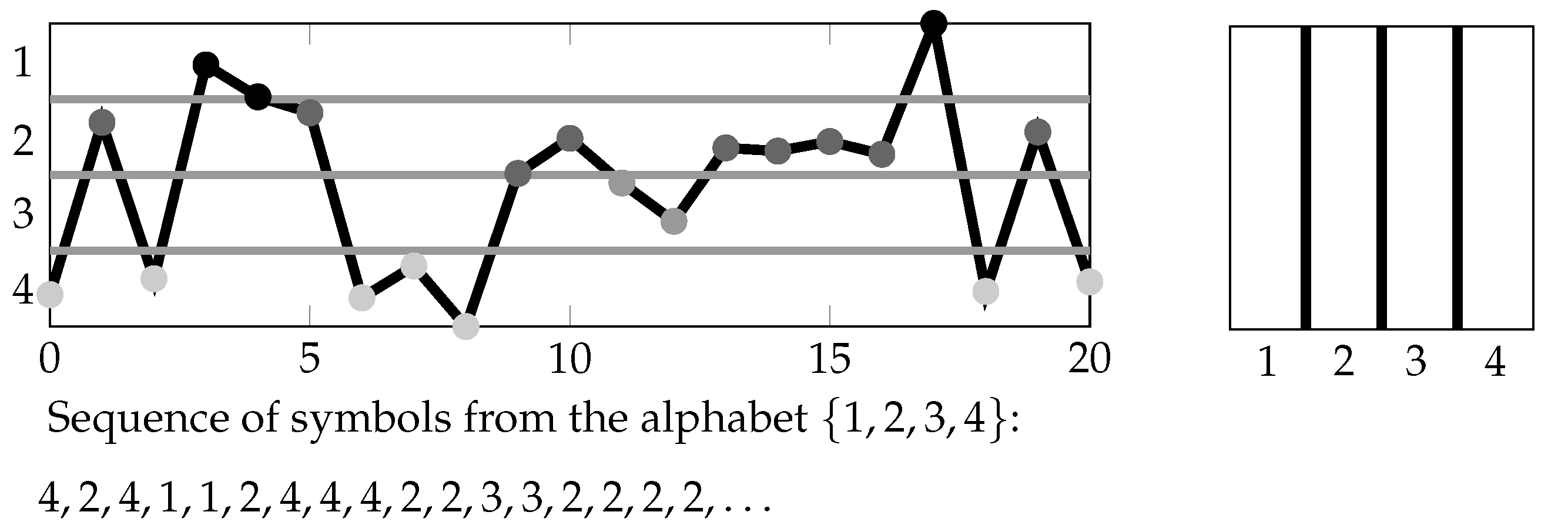
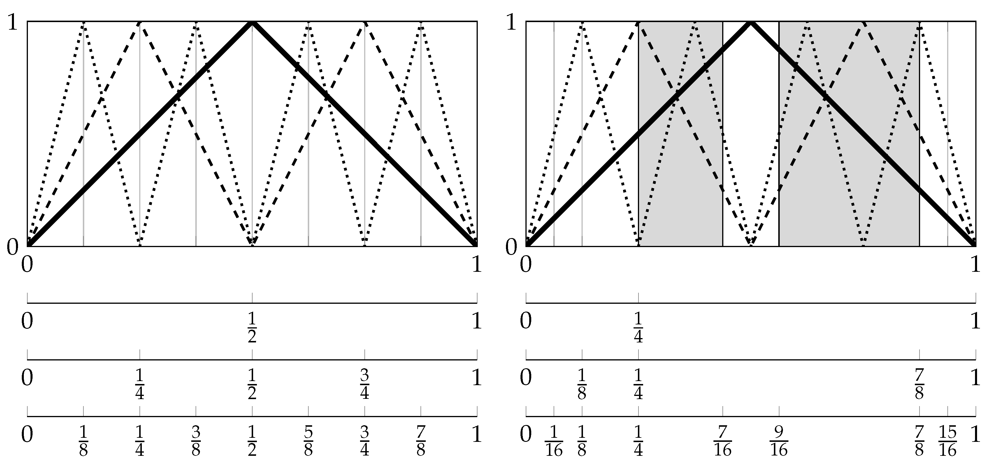
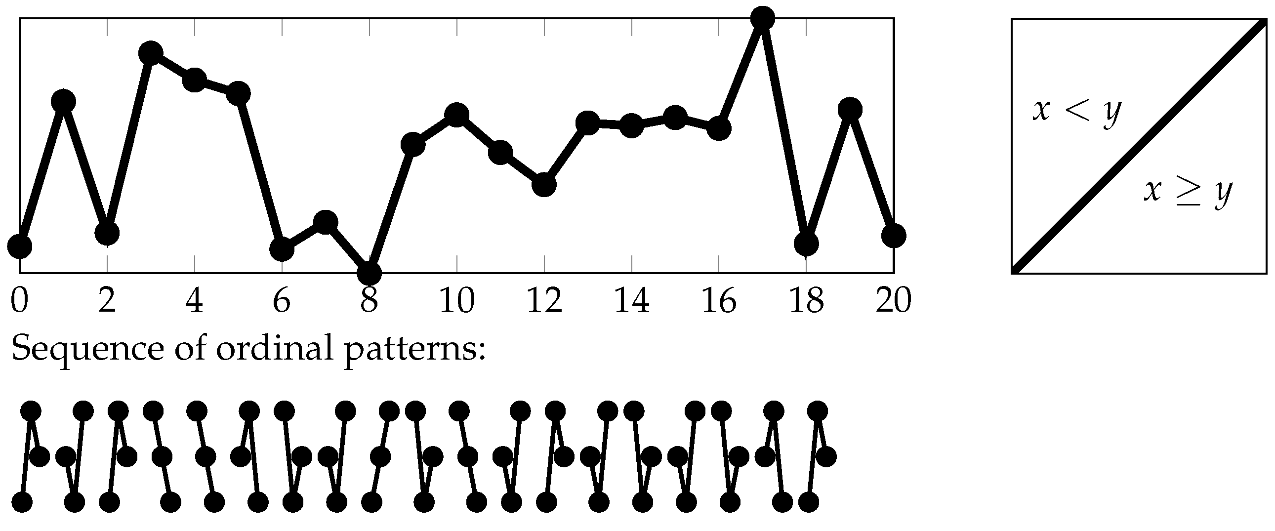
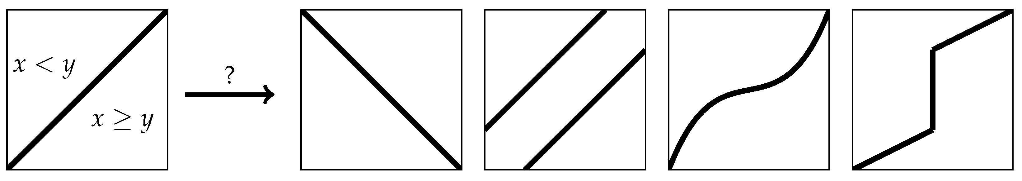
1.4. A “Two-Dimensional” Way of Symbolizations

The partitions C d with d N that we want to study in the following are formed on the basis of a finite partition R of the two-dimensional Euclidean space R 2 and finite sets E d N 0 × N 0 of time pairs:
C d = C R , E d ( T , X ) : = i = 1 n ( s , t ) E d X i T s , X i T t 1 ( R ) A ,
i.e., C d is the coarsest partition refining all partitions:
X i T s , X i T t 1 ( R ) = ω Ω X i ( T s ( ω ) ) , X i ( T t ( ω ) ) R R R
for ( s , t ) E d (see Section 4.1 for the definition of the join r = 1 m C r of finite partitions C r A of Ω ).
Here, R specifies the symbolization scheme for classifying the mutual position of measurements by X i at two times s and t (see Figure 1 and Figure 2, as well as the next section). We call R the basic symbolization scheme in the following. Note that we display the two-dimensional Euclidean space R 2 by a square for illustrative purposes.
Further, the choice of ( E d ) d N complies with Definition 1, in particular in order to realize that C d + 1 refines C d (see Section 4.1), C d is finite (see Definition 1(i)), and each time point that is relevant for the symbolization is accessed (see Definition 1(ii)).
Definition 1.
We call a sequence ( E d ) d N of sets E d with E 1 E 2 { ( s , t ) s , t N 0 , s < t } a timing if there exists a set { v 0 , v 1 , } N 0 with v 0 < v 1 < v 2 < such that:
(i) 
for each d N , it holds E d { v 0 , v 1 , , v d } 2 , and
(ii) 
for each s { v 0 , v 1 , , v d } , there exists some t { v 0 , v 1 , , v d } such that ( s , t ) E d or ( t , s ) E d .
A timing is for instance given by the sets:
E d = ( s , t ) s , t 0 , 1 , 2 , , d with s < t ; d N ,
or by (11) and (17) (see below). It is suggestive to call the timing defined by (9) full timing in the following.
Subsequently, we discuss the following two questions:
  • Why is the approach given natural and sufficiently general?
  • Under which conditions on the basic symbolization scheme R and the timing E d does the sequence ( C d ) d N = C R , E d ( T , X ) d N satisfy Statement (5) or even (4)?
Section 2 is devoted to the first question. In the first part of Section 3, we summarize our results to the second question and give some examples of basic symbolization schemes. Sufficient conditions that answer the second question including known results are presented for the interested reader in the second part of Section 3 and proven in Section 4 (see also the Appendix). We close this paper with some remarks about further theoretical and practical scientific issues (see Section 5).

2. Two Examples

At first glance, the above approach gives a rather exaggerated impression. The aim of the following examples is to convince the reader that sequences ( C d ) d N formed on the basis of basic symbolization schemes R and timings ( E d ) d N are natural and are unifying known symbolic approaches.

2.1. “Classical” Symbolic Dynamics

First, we discuss “classical” symbolic dynamics with a fixed partition (see for instance Daw et al. [1], Kurths et al. [13] and the references given therein). For convenience, we assume that the dynamics is living on the real line, i.e., Ω = R , and restrict ourselves to the simple case that R is subdivided into a finite number of intervals I 1 , I 2 , , I k (see for instance Figure 1).
The determination of the entropy rate of the partition C = { I 1 , I 2 , , I k } is based on the partitions:
( C ) t = { C ( a 1 , a 2 , , a t ) a 1 , a 2 , , a t { 1 , 2 , , k } }
increasing with t N , where:
C ( a 1 , a 2 , , a t ) = { ω Ω ω I a 1 , T ( ω ) I a 2 , , T t 1 ( ω ) I a t }
consists of those states ω Ω successively visiting I a 1 , I a 2 , , I a t , i.e., having the symbolic itinerary a 1 , a 2 , , a t . Compare to Section 4.1, in particular for the deliberate notation used in this subsection, and see Figure 3, where we illustrate the symbolization process underlying the determination of the entropy rate for t = 3 .
For all t N , it holds:
( C ) t = s = 0 t 1 ( T s ) 1 ( C ) .
In order to rewrite the “classical” approach into a form compatible with the proposed one, we need an artificial two-dimensional “blow-up” of the partitions ( C ) t ; t N , which is given by the partition:
R : = { I 1 × R , I 2 × R , , I k × R } ( see Figure   1 ) ,
of R 2 and the sets of time pairs:
E t : = { ( 0 , 1 ) , ( 1 , 2 ) , ( 2 , 3 ) , , ( t 1 , t ) } ; t N ,
that is:
( C ) t = s = 0 t 1 ( X T s ) 1 ( ( C ) 1 ) = ( s , u ) E t ( X T s , X T u ) 1 ( R ) = C R , E t ( T , X ) .
Here, we consider, motivated by our general procedure, the single observable X (meaning X = X in the general framework) with X ( ω ) = ω for all ω Ω , which fits the situation described at the end of Section 1.3.
This means in the other direction that the partitions C d = C R , E d ( T , X ) are coinciding with the partitions ( C ) d . In particular, it holds:
h μ ( T , C d ) = h μ ( T , ( C ) d )
for all d N , and since h μ ( T , ( C ) t ) = h μ ( T , C ) for all t N (see for instance Einsiedler and Schmidt [14], Satz 3.13), we obtain:
h μ ( T , C d ) = h μ ( T , C )
for all d N . This fact implying that the sequence ( C d ) d N = C R , E d ( T , X ) d N is generating iff C is generating under T (see the final remarks in Section 4.1) says that R as given by (10) has no generating potential when C fails to be generating under T. This is not surprising since R is no more than a two-dimensional “blow-up” of C . The second example shows the existence of good choices of R with generating properties under certain assumptions.
In Figure 4, we study (compare to Section 4.1) two different initial partitions, that is C = { [ 0 , 1 / 2 ) , [ 1 / 2 , 1 ) } and D = { [ 0 , 1 / 4 ) , [ 1 / 4 , 1 ) } , under the transformation T : ( [ 0 , 1 ) ) , defined by:
T ( ω ) = 2 ω if 0 ω < 1 2 , 2 2 ω if 1 2 ω < 1 ,
i.e., T is the full tent map on Ω : = [ 0 , 1 ) . The KS entropy is ln ( 2 ) (see for instance Bollt et al. [5] and the references given therein), and in fact, it holds:
H μ ( C ) = 1 2 H μ ( ( C ) 2 ) = 1 3 H μ ( ( C ) 3 ) = = 1 t H μ ( ( C ) t ) = = ln ( 2 ) ,
whereby:
H μ ( D ) = 1 4 ln ( 1 4 ) 3 4 ln ( 3 4 ) < ln ( 2 )
(see Section 4.1). Since 1 t H μ ( ( C ) t ) decreases to h μ ( T , C ) for any finite partition C A of Ω (see Walters [10], Chapter 4) and by Theorem 4.18 of [10] (see Equation (1)), we have by C a generating and by D a non-generating (misplaced) partition under T (see Bollt et al. [5] and Steuer et al. [7] for detailed information about possible consequences if a non-generating partition is used in time series analysis, as well as Figure 7).

2.2. Ordinal Symbolic Dynamics

Ordinal symbolic dynamics is a relatively new symbolic approach going back to Bandt and Pompe [15] and applied in various fields (see for instance Zanin et al. [2], Amigó et al. [3] and the references given therein). The idea of the symbolization scheme is to partition the state space according to ordinal patterns of orders d N . For fixed d and a random vector X = ( X i ) i = 1 n , two states ω 1 , ω 2 Ω belong to the same part of a partition if for each i = 1 , 2 , , n , the observable X i provides the same order relations on the orbits of length d + 1 of ω 1 and ω 2 :
For all s , t with 0 s < t d , it holds:
X i ( T s ( ω 1 ) ) X i ( T t ( ω 1 ) )   iff   X i ( T s ( ω 2 ) ) X i ( T t ( ω 2 ) ) .
One easily sees that the obtained partitions can be written in the form C d = C R , E d ( T , X ) with:
R = ( x , y ) R × R x y , ( x , y ) R × R x < y ( see Figure 2 )
and the full timing (see Equation (9)).
The sequence ( C d ) d N is obviously increasing. Antoniouk et al. [16] show the following statement for R as given by (13) and the full timing ( E d ) d N given by (9), here formulated in the language of our general approach:
If   T   is   ergodic   and   X   satisfies   ( 6 )   or   weaker   ( 7 ) ,   then ( C d ) d N = C R , E d ( T , X ) d N   is   generating ,   hence   h μ KS ( T ) = lim d h μ ( T , C d ) = sup d N h μ ( T , C d ) .
Unlike the “classical” approach, the basic symbolization scheme R , as given by (13), regards a kind of dependency between two measurements by X i . The statement (14) shows the substantial difference between “classical” and ordinal symbolic dynamics: by using R as given in (13), we obtain a generating sequence ( C d ) d N , regardless of whether C 1 = C is generating under T.

2.3. An Extension of Ordinal Symbolic Dynamics

In the rest of the paper, we discuss for which R and ( E d ) d N the statement (14) remains true; whereby, this section is dedicated to those readers who are mainly interested in the idea and results of our study. Since the corresponding considerations to validate our subsequent statement are fairly technical and due to even more general results, we refer here only to the statements and proofs in the later discussion (Section 3 and the Appendix). First of all, obviously, (14) remains true when R is substituted by a refinement of (13) (see Figure 5). Moreover, in the case that Ω is a Borel subset of R n and X i , i = 1 , 2 , , n is the i-th coordinate projection (see the closing remarks of Section 1.3), as well as μ ( A ) > 0 for all open subsets A of Ω , Statement (14) remains true if we modify R even more (see the closing remarks of Section 3.1):
Theorem 1.
Let Ω be a Borel subset of R n and X i ; i = 1 , 2 , , n be the i-th coordinate projection. Further, let R be a basic symbolization scheme defined by:
R = ( x , y ) R × R g ( x ) y , ( x , y ) R × R g ( x ) < y ,
or finer, where g : R is a one-to-one B ( R ) - B ( R ) measurable map with B ( R ) being the Borel σ-algebra on R (see for instance Figure 6). If μ ( A ) > 0 for all open subsets A of Ω, then for the full timing ( E d ) d N (see Equation (9)), Statement (14) is fulfilled.

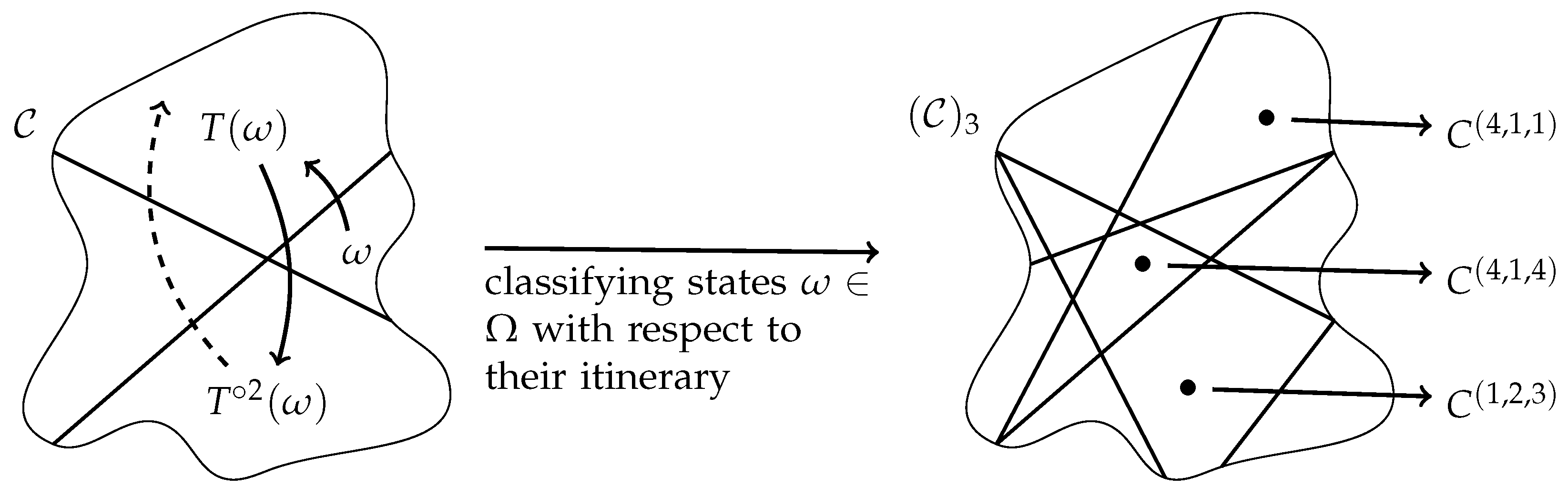
3. Main Mathematical Results

Antoniouk et al. [16] show that the search for a generating partition under T can be bypassed by choosing ordinal symbolic dynamics. It namely provides, in the ergodic case and if X satisfies (6) or weaker (7), a generating sequence of finite partitions by default, that is the generating property is valid regardless of the properties of the original system considered (see Statement (14) in Section 2.2).
The question arises if other symbolic approaches deliver similar results. In fact, by generalizing the ideas and results of Antoniouk et al. [16], we give sufficient conditions on R and ( E d ) d N for (14). This we present the interested reader in the next sections.

3.1. Preserving the Information of Observables

The following is quite technical, but shows under which conditions the information given by the observables is preserved if basic symbolization schemes R such as given by (15), or finer, are considered. Hence, if Theorem 2 holds and A μ σ ( X ) , then ( C d ) d N is generating.
Theorem 2.
Let T be ergodic, X = ( X i ) i = 1 n a random vector, R a basic symbolization scheme, ( E d ) d N a timing and ( C d ) d N a sequence of finite partitions constructed from R and ( E d ) d N (see Equation (8)). If further:
(i) 
g is admissible with respect to X i for all i = 1 , 2 , , n ,
(ii) 
F X i is admissible with respect to g X i for all i = 1 , 2 , , n and
(iii) 
g X i X i T t σ C R , E d ( T , X i ) d N for all i = 1 , 2 , , n and t N 0 ,
then:
σ ( X ) μ σ ( ( C d ) d N ) .
We call a function ϕ : R admissible with respect to a random variable Y on Ω if σ ( Y ) μ σ ( ϕ Y ) ; this is for example the case if ϕ is a one-to-one B ( R ) - B ( R ) measurable map (see the closing remarks of the Appendix on one-to-one maps and Lemma A3 for general conditions on ϕ such that ϕ is admissible). Requiring that F X i has to be admissible with respect to g X i means that g has to be constructed in such a way that:
σ ( g X i ) μ σ ( F X i g X i )
holds (compare to the proof of Lemma A3 and subsequent remarks). This assumption is redundant if Ω is a Borel subset of R n ; each X i ; i = 1 , 2 , , n is the i-th coordinate projection (see the closing remarks of Section 1.3); and μ ( A ) > 0 for all open subsets A of Ω , because then, F X i is one-to-one (see the closing remarks of the Appendix on one-to-one maps). Finally, note that symbolizations based on R as given by (15), or finer, have the property (iii) of Theorem 2 (in particular, compare (iii) of Theorem 2 to the structure of (15)). Summarizing, the assumptions of Theorem 2 are generalizations of the assumptions of Theorem 1, and thus, Theorem 1 follows by Theorem 2.

3.2. Preserving the Information of the Measuring Process

In this section, we state sufficient conditions such that the information given by the measuring process is preserved. Therefore, if these conditions are fulfilled and A μ σ X T t t N , then ( C d ) d N is generating. Define:
C R , E d ( T , Y ) : = i = 1 n ( s , t ) E d Y i T s , Y i T t 1 ( R ) A ,
where Y = ( Y i ) i = 1 n is an arbitrary random vector (compare to Equation (8)), and consider the special case Y = ( Y i ) i = 1 n = X T l = X i T l i = 1 n for some l N in the following.
Definition 2.
Let R be a basic symbolization scheme and ( E d ) d N be a timing. We call the tuple ( R , ( E d ) d N ) consistent if for all t > 1 and d N , it holds:
s = 0 t 1 C R , E d ( T , X T s ) s = 0 t 2 C R , E d + 1 ( T , X T s ) .
Compare to Keller et al. [17], who regard the ordinal approach: observe that, in the consistent case, by applying (16) repeatedly, one shows that:
s = 0 t 1 C R , E d ( T , X T s ) C R , E d + t 1 ( T , X )
for all t, d N . Consistency ensures that for all t N 0 , it holds:
σ C R , E d ( T , X T t ) d N σ ( ( C d ) d N ) .
In other words, if the information given by a measurement at a time t N is preserved by C R , E d ( T , X T t ) d N , then it also is preserved by ( C d ) d N (compare to the proof of Theorem 3).
Consistency depends on the interplay of the underlying system, the considered random vector X = ( X i ) i = 1 n , R and ( E d ) d N ; however, a skillful choice of the timing guarantees that ( R , ( E d ) d N ) is consistent independent of the system and X . This we discuss in Section 4.3. Note here that ( R , ( E d ) d N ) is always consistent if ( E d ) d N is the full timing (see Equation (9)); however, the tuple is not consistent in general if a timing given by:
E d = ( 0 , t ) t 0 , 1 , 2 , , d ; d N
is considered.
Theorem 3.
Let X = ( X i ) i = 1 n be a random vector, R a basic symbolization scheme, ( E d ) d N a timing and ( C d ) d N a sequence of finite partitions constructed by R and ( E d ) d N (see Equation (8)). If further:
(i) 
σ ( X ) μ σ ( ( C d ) d N ) and
(ii) 
( R , ( E d ) d N ) is consistent,
then:
σ X T t t N μ σ ( ( C d ) d N ) .
Recall that (i) of Theorem 3 particularly holds if Conditions (i)–(iii) of Theorem 2 are fulfilled.

4. Proofs

We begin by summarizing some basic notations and concepts. Thereafter, we prove Theorem 2 and Theorem 3, whereby quite technical and complicated lemmas can be found in the Appendix.

4.1. Preliminaries

Our whole discussion is concerned with finite partitions C A of Ω and with sequences of finite partitions ( C d ) d N . A finite partition C of Ω is a set system:
C : = C ( 1 ) , C ( 2 ) , , C ( q ) A ; q N ,
where:
l = 1 q C ( l ) = Ω and C ( l ) C ( k ) = for any l k { 1 , 2 , , q } .
Particularly, we are interested in such sequences that are increasing, meaning that C d + 1 is finer than C d for all d N :
A partition D = D ( 1 ) , D ( 2 ) , , D ( p ) is finer than a partition C = C ( 1 ) , C ( 2 ) , , C ( q ) ; we write C D , or, equivalently, C is coarser than D if for all l { 1 , 2 , , q } there exists a nonempty K { 1 , 2 , , p } such that:
C ( l ) = k K D ( k ) .
Moreover, we consider the join r = 1 m C r of finite partitions C r A of Ω with m N and r = 1 , 2 , , m , which is defined by:
r = 1 m C r = r = 1 m C r ( l r ) | l r { 1 , 2 , , | C r | }   for   r = 1 , 2 , , m ,
that is the coarsest partition refining all C r .
Furthermore, sub- σ -algebras of A are central to us, especially the ones σ ( M ) generated by subsets M of A , i.e., the smallest sub- σ -algebra containing M :
σ ( M ) = F A is σ algebra and M F F .
We consider also the join of σ -algebras F i A ; i I defined by:
i I F i = σ i I F i .
Overall, we have a special interest in the following sub- σ -algebras of A :
σ ( ( C d ) d N ) = d N σ ( C d )
for ( C d ) d N being a finite partition sequence of Ω ,
σ ( X ) = i = 1 n σ ( X i ) = i = 1 n X i 1 ( B ) B B ( R ) , σ ( X T s ) = i = 1 n σ ( X i T s ) = i = 1 n ( X i T s ) 1 ( B ) B B ( R ) , σ X T t t N 0 = t N 0 σ X T t = i = 1 n t N 0 σ X i T t
for X = ( X i ) i = 1 n being a random vector on Ω and s N .
We close this subsection by giving an exact definition of the entropy rate h μ ( T , C ) of a finite partition C (see Figure 3): one assigns to every part C ( i ) of the partition C = C ( 1 ) , C ( 2 ) , , C ( q ) the letter i of the alphabet A = { 1 , 2 , , q } . Each word ( a 1 , a 2 , , a t ) of length t N over A defines a set:
C ( a 1 , a 2 , , a t ) = ω Ω | ω , T ( ω ) , , T t 1 ( ω ) C ( a 1 ) × C ( a 2 ) × × C ( a t ) .
All non-empty sets C ( a 1 a 2 a t ) provide a partition ( C ) t A of Ω . We use the notation ( C ) t to emphasize that the partition is constructed with respect to T. In particular, ( C ) 1 = C . The entropy rate of T with respect to C is given by:
h μ ( T , C ) = lim t 1 t H μ ( ( C ) t ) = lim t H μ ( ( C ) t ) H μ ( ( C ) t 1 ) ,
where H μ ( ( C ) t ) is the Shannon entropy of ( C ) t , that is for a finite partition D = D ( 1 ) , D ( 2 ) , , D ( p ) :
H μ ( D ) = l = 1 p μ ( D ( l ) ) ln ( μ ( D ( l ) ) ) ( with 0 ln ( 0 ) : = 0 ) .
For a fuller treatment, e.g., for statements that the limit in Equation (18) exists and 1 t H μ ( ( C ) t ) , as well as H μ ( ( C ) t ) H μ ( ( C ) t 1 ) decreases to h μ ( T , C ) , we refer the reader to Chapter 4 of Walters [10]. Note that for all t N , it holds ( C ) t 1 ( C ) t , and:
H μ ( ( C ) t ) H μ ( ( C ) t 1 ) 1 t s = 1 t H μ ( ( C ) s ) H μ ( ( C ) s 1 ) = 1 t H μ ( ( C ) s ) .
Moreover, we say that C is generating under T if:
A μ σ ( ( ( C ) t ) t N ) .
If we consider instead an arbitrary sequence of finite partitions ( C d ) d N for which:
A μ σ ( ( C d ) d N )
holds, then we call ( C d ) d N just generating.

4.2. Proof of Theorem 2

In order to prove Theorem 2, we generalize the results of Antoniouk et al. [16] (Lemmas 3.2, 3.3 and Corollary 3.4) and extend their proofs. Thereby, we utilize properties of the distribution function F X i : R [ 0 , 1 ] of a random variable X i : Ω R , i.e.,
F X i ( a ) = μ ( { ω Ω X i ( ω ) a } )
for all a R (see Lemmas A1 and A2 in the Appendix) and show:
σ ( X i ) μ σ C R , E d ( T , X i ) d N
by the detour:
σ ( X i ) μ σ ( g X i ) μ σ ( F X i g X i ) μ σ C R , E d ( T , X i ) d N .
Proof of Theorem 2.
Note that it is enough to show that:
σ ( X i ) μ σ C R , E d ( T , X i ) d N
holds for all i = 1 , 2 , , n since the sub- σ -algebras σ C R , E d ( T , X i ) d N generate the sub- σ -algebra:
σ ( ( C d ) d N ) = σ C R , E d ( T , X ) d N .
Thus, let us regard i N as fixed. By the assumptions Theorem 2(i) and (ii) (compare also to Lemma A3), we obtain:
σ ( X i ) μ σ ( g X i ) μ σ ( F X i g X i ) .
Moreover, by Theorem 2(iii) and Lemma A2, we have that:
σ ( F X i g X i ) μ σ C R , E d ( T , X i ) d N .
Hence:
σ ( X i ) μ σ C R , E d ( T , X i ) d N ,
which completes the proof. ☐

4.3. Proof of Theorem 3

The main additional property needed in Theorem 3 is that ( R , ( E d ) d N ) is consistent (see Definition 2). In order to see how a timing has to be constructed such that ( R , ( E d ) d N ) is generally consistent, let us regard t , d N as fixed and consider states ω 1 , ω 2 Ω , which are in different parts of:
s = 0 t 1 C R , E d ( T , X T s ) .
Then, there exists at least one s { 0 , 1 , , t 1 } , one i = 1 , 2 , , n and a time pair ( u , v ) E d such that:
X i ( T s + u ( ω 1 ) ) , X i ( T s + v ( ω 1 ) ) and X i ( T s + u ( ω 2 ) ) , X i ( T s + v ( ω 2 ) )
are in different parts of R . If now for any s { 0 , 1 , , t 1 } and ( u , v ) E d , it holds that ( s + u , s + v ) E d + t 1 , then:
X i T s + u , X i T s + v 1 ( R ) C d + t 1 .
Hence, ( R , ( E d ) d N ) is consistent if the previous holds for all t , d N .
Proof of Theorem 3.
Compare to [16] (Corollary 3.5). By Theorem 3(ii), i.e., ( R , ( E d ) d N ) is consistent, it holds:
C R , E d ( T , X T ) C R , E d + 1 ( T , X )
for all d N . These refinements imply:
σ C R , E d ( T , X T t ) d N σ ( ( C d ) d N )
for all t N 0 (see Walters [10], Chapter 4, Section 1). Moreover, by Theorem 3(i), it holds:
σ X T t μ σ C R , E d ( T , X T t ) d N
for all t N 0 . Hence:
σ X T t t N 0 μ σ ( ( C d ) d N ) ,
which proves the theorem. ☐

5. Some Remarks

In proposing and studying our universal symbolic approach toward KS entropy, we have restricted ourselves to the kernel ideas. In particular, we have attached importance to point out that a “two-dimensional” symbolization, that is linking two observations, can provide a better basic symbolization scheme than symbolizing only on a one-dimensional observational level. The obtained results can be simply generalized in two directions:
On the one hand, infinitely many observables instead of finitely many ones can be considered. Here, the results obtained by Keller et al. [18] (see also the references given in the paper) can directly be adapted, which leads to a description of the KS entropy by a double limit substituting the limit in (2). On the other hand, some of our results remain true when relaxing ergodicity by some rather general conditions on the dynamics considered. For this, the ergodic decomposition theorem can be utilized. We refer to the discussion in Keller et al. [18] and the references given therein.
Our study does not touch aspects as the speed of convergence in (2), as a general comparison of basic symbolic schemes and as an entropy estimation, which are, incontestably, very interesting both from the theoretical and practical viewpoint. Our approach provides some theoretical framework within concrete methods for time series and system analysis and can be specified in accordance with requirements given in practice.
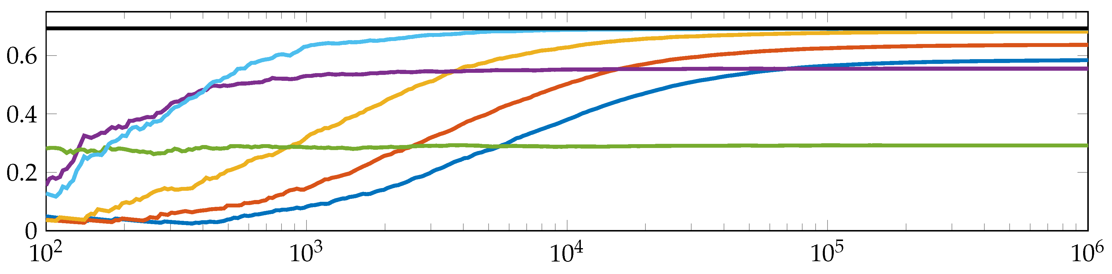
In order to give a brief perspective on the matter, we decoded a finite orbit ( x t ) t = 0 T ; T N of the tent map (see Section 2.1), that is:
x t + 1 = 2 x t if 0 x t < 1 2 , 2 2 x t if 1 2 x t < 1
for all t = 0 , 1 , , T 1 and x 0 uniformly distributed, into a sequence of symbols, fixed a word length t N and naively estimated the difference H μ ( ( C ) t ) H μ ( ( C ) t 1 ) by replacing the probabilities by relative frequencies of symbol word occurrences.
Figure 7 shows the results for different t N and symbolization schemes in dependence of the orbit length T , here between 10 2 and 10 6 . We chose to take the difference because of (19), i.e., the difference for fixed t is a better approximation of the entropy rate h μ ( T , C ) than 1 t H μ ( ( C ) t ) . For a fuller treatment, we refer the reader to Keller et al. [19], in particular for more information of how to construct a symbol sequence with respect to ordinal symbolic dynamics with fixed order d N and word length t N .
Clearly, Figure 7 emphasizes common problems of time series analysis, which have to be faced, as, for example, the trade-off between computational capacity and computation accuracy, which includes undersampling problems, the choice of parameters, stationarity assumptions, and so forth (see for instance Keller et al. [19]). A discussion of all these aspects would be beyond the scope of this paper, but is planned for the future.

Acknowledgments

We acknowledge financial support by Land Schleswig-Holstein within the funding program Open Access Publikationsfonds.

Author Contributions

Inga Stolz and Karsten Keller jointly conceived and discussed the presented ideas. Inga Stolz developed the theory and performed the numerical simulations. Karsten Keller supervised the course of action and findings. Both authors contributed materially to the paper and read as well as approved the final manuscript.

Conflicts of Interest

The authors declare no conflict of interest.

Appendix A

Lemma A1.
Let X, Y : Ω R be two random variables, F X : R [ 0 , 1 ] the distribution function of X and I d X , Y : Ω [ 0 , 1 ] be the counting map of X and Y, given by:
I d X , Y ( ω ) : = 1 d t = 1 d 1 X T t Y ( ω )
for all ω Ω . If T is ergodic, then:
lim d I d X , Y = F X Y μ a l m o s t e v e r y w h e r e .
Proof of Lemma A1.
Let A a = X 1 ( ( , a ] ) for any a R . By Birkhoff’s ergodic theorem (see for instance Walters [10]), there exists a set N a Ω such that μ ( N a ) = 0 and:
F X ( a ) = μ ( A a ) = lim d 1 d t = 1 d 1 { X T t a } ( ω )
for any a R and ω Ω N a . Let B be a countable dense subset of R such that it includes all a R for which F X is discontinuous, and let N = a B N a . Then, μ ( N ) = 0 , and Equation (A1) holds for each a B and ω Ω N . Our next claim is that for all ω Ω N , it holds:
lim d I d X , Y ( ω ) = F X ( Y ( ω ) ) .
By (A1), this is true if ω Ω N satisfies a : = Y ( ω ) B . It is moreover true if ω Ω N and a : = Y ( ω ) R B , which we show in the following:
Let ( b i ) i N and ( c i ) i N be two sequences converging to a with:
b i B ( , a ) and c i B ( a , )
for all i N . Hence, b i < a < c i , and for all i N , it holds:
F X ( b i ) = lim d 1 d t = 1 d 1 { X T t b i } ( ω ) and F X ( c i ) = lim d 1 d t = 1 d 1 { X T t c i } ( ω )
since ω Ω N . Thus, for all d N , we have:
t = 1 d 1 { X T t b i } ( ω ) t = 1 d 1 { X T t Y } ( ω ) t = 1 d 1 { X T t c i } ( ω ) .
Furthermore, since F X is continuous at a, we obtain:
F X ( a ) = lim i F X ( b i ) lim inf d I d X , Y lim sup d I d X , Y lim i F X ( c i ) = F X ( a ) .
Hence, we can summarize that for all ω Ω N , it holds lim d I d X , Y ( ω ) = F X ( Y ( ω ) ) , which is the desired conclusion. ☐
Lemma A2.
Let X = ( X i ) i = 1 n and Y = ( Y i ) i = 1 n be two random vectors. If T is ergodic and:
Y i X i T t σ C R , E d ( T , X i ) d N
for all i = 1 , 2 , , n and t N 0 , then:
σ ( ( F X i Y i ) i = 1 n ) μ σ ( ( C d ) d N ) .
Proof of Lemma A2.
Since the sub- σ -algebras σ C R , E d ( T , X i ) d N generate the sub- σ -algebra:
σ ( ( C d ) d N ) = σ C R , E d ( T , X ) d N ,
it is enough to show that for all i = 1 , 2 , , n , it holds:
σ ( F X i Y i ) μ σ C R , E d ( T , X i ) d N .
Hence, let us regard i as fixed. By the assumption given, that is:
Y i X i T t σ C R , E d ( T , X i ) d N
for all t N o , it holds that I d X i , Y i is σ C R , E d ( T , X i ) d N - B ( [ 0 , 1 ] ) -measurable for any d N (see for instance Billingsley [20], remarks on simple real functions in Section 13). Hence:
σ I d X i , Y i d N σ C R , E d ( T , X i ) d N .
Moreover, the limit of I d X i , Y i as d approaches infinity exists for each ω Ω since I d X i , Y i I d + 1 X i , Y i and 0 I d X i , Y i 1 , hence:
σ lim d I d X i , Y i σ I d X i , Y i d N
(see for instance Billingsley [20], Theorem 13.4.(ii)). Furthermore, by Lemma A1, there exists a set N Ω with μ ( N ) = 0 such that:
lim d I d X i , Y i ( ω ) = F X i ( Y i ( ω ) )
for all ω Ω N . Hence, for any B B ( [ 0 , 1 ] ) , it holds:
μ ( F X i Y i ) 1 ( B ) lim d I d X i , Y i 1 ( B ) μ ( N ) = 0 ,
which gives:
σ ( F X i Y i ) μ σ I d X i , Y i d N ,
and the lemma follows. ☐
The following lemma yields sufficient conditions for (i) and (ii) of Theorem 2.
Lemma A3.
Let X : ( Ω , A , μ ) ( R , B ( R ) ) be a random variable, ϕ : R a B ( R ) - B ( R ) a measurable map and G a family of subsets of R that generates the Borel σ-algebra B ( R ) . If ϕ has the two properties:
(i) 
ϕ ( G ) B ( R ) and
(ii) 
μ X 1 ϕ 1 ϕ ( G ) G = 0
for all G G , then σ ( X ) μ σ ( ϕ X ) .
Proof of Lemma A3.
Since G generates B ( R ) , it holds that σ ( X ) is generated by the sets X 1 ( G ) (see for instance Elstrodt [21], Kapitel 1, Satz 4.4). Hence, the Lemma is proven if for any G G , there exists some G σ ( ϕ X ) such that μ X 1 ( G ) G = 0 . In order to show this, choose:
G = X 1 ϕ 1 ϕ ( G ) = ( ϕ X ) 1 ϕ ( G ) .
By Lemma A3(i), it holds that G σ ( ϕ X ) , and by (ii), we see that:
μ X 1 ( G ) G = μ X 1 ( ϕ 1 ϕ ( G ) ) G = 0 ,
which completes the proof. ☐
Note that since ϕ is a B ( R ) - B ( R ) measurable map in Lemma A3, it holds in particular:
σ ( X ) σ ( ϕ X )
for any random variable X : Ω R : Let A σ ( ϕ X ) , then:
A = ( ϕ X ) 1 ( B ) = X 1 ϕ 1 ( B )
for some B B ( R ) . Hence, by ϕ 1 ( B ) B ( R ) , it follows that A σ ( X ) .
Lemma A3 is evident if ϕ is a one-to-one B ( R ) - B ( R ) measurable map since then:
ϕ 1 ϕ ( B ) B =
and ϕ ( B ) B ( R ) for all B B ( R ) (see for instance Cantón et al. [22]); nevertheless, it also includes self-maps such as the distribution function F X of a random variable X (see Antoniouk et al. [16], Lemma 3.2), i.e.,
σ ( X ) μ σ ( F X X ) :
Let G = { ( , a ) a R } ; since F X is increasing, Lemma A3(i) holds for all G G . Assumption Lemma A3(ii) is proven by Antoniouk et al. [16] (Lemma 3.1(3)) by showing firstly that:
F X 1 F X ( ( , a ) ) ( , a )
coincides either with the interval [ a , a * ] or with [ a , a * ) for any a R , where a * = sup F X 1 F X ( a ) and subsequently that μ X 1 ( [ a , a * ] ) = 0 . Hence, the inclusion (compare to Theorem 2(ii)):
σ ( g X ) μ σ ( F X g X ) ,
where g : R is a self-map, holds if we obtain:
μ ( X 1 g 1 ( [ a , a * ] ) ) = 0
for any a R . This is true if, for instance, either F X is one-to-one or g ( ω ) = ω for all ω Ω where F X is not one-to-one.

References

  1. Daw, C.S.; Finney, C.E.A.; Tracy, E.R. A review of symbolic analysis of experimental data. Rev. Sci. Instrum. 2003, 74, 915–930. [Google Scholar] [CrossRef]
  2. Zanin, M.; Zunino, L.; Rosso, O.A.; Papo, D. Permutation Entropy and Its Main Biomedical and Econophysics Applications: A Review. Entropy 2012, 14, 1553–1577. [Google Scholar] [CrossRef]
  3. Amigó, J.M.; Keller, K.; Unakafova, V.A. Ordinal symbolic analysis and its application to biomedical recordings. Phil. Trans. R. Soc. A 2015, 373, 20140091. [Google Scholar] [CrossRef] [PubMed]
  4. Crutchfield, J.P.; Packard, N.H. Symbolic dynamics of noisy chaos. Phys. D: Nonlinear Phenom. 1983, 7, 201–223. [Google Scholar] [CrossRef]
  5. Bollt, E.M.; Stanford, T.; Lai, Y.-C.; Życzkowski, K. What symbolic dynamics do we get with a misplaced partition?: On the validity of threshold crossings analysis of chaotic time-series. Phys. D: Nonlinear Phenom. 2001, 154, 259–286. [Google Scholar] [CrossRef]
  6. Kennel, M.B.; Buhl, M. Estimating Good Discrete Partitions from Observed Data: Symbolic False Nearest Neighbors. Phys. Rev. Lett. 2003, 91, 084102. [Google Scholar] [CrossRef] [PubMed]
  7. Steuer, R.; Molgedey, L.; Ebeling, W.; Jiménez-Montaño, M.A. Entropy and optimal partition for data analysis. Eur. Phys. J. B 2001, 19, 265–269. [Google Scholar] [CrossRef]
  8. Letellier, C. Symbolic sequence analysis using approximated partition. Chaos, Solitons & Fractals 2008, 36, 32–41. [Google Scholar]
  9. Li, Y.; Ray, A. Unsupervised Symbolization of Signal Time Series for Extraction of the Embedded Information. Entropy 2017, 19, 148. [Google Scholar] [CrossRef]
  10. Walters, P. An Introduction to Ergodic Theory; Springer: New York, NY, USA, 1981. [Google Scholar]
  11. Takens, F. Detecting strange attractors in turbulence. In Lecture Notes in Mathematics, Proceedings of a Symposium Held at the University of Warwick 1979/80, Coventry, UK, 1980; Rand, D., Young, L.S., Eds.; Springer: Berlin/Heidelberg, Germany, 1981; Volume 898, pp. 366–381. [Google Scholar]
  12. Gutman, Y. Takens’ embedding theorem with a continuous observable. In Ergodic Theory: Advances in Dynamical Systems; Assani, I., Ed.; Walter de Gruyter: Berlin/Heidelberg, Germany, 2016; pp. 134–141. [Google Scholar]
  13. Kurths, J.; Schwarz, U.; Witt, A.; Krampe, R.T.; Abel, M. Measures of complexity in signal analysis. In Proceedings of the AIP Conference: Chaotic Fractal and Nonlinear Signal Processing, 3rd Technical Conference on Nonlinear Dynamics (Chaos) and Full Spectrum Processing, New London, CT, USA, 10–13 July 1995; Volume 375, pp. 33–54. [Google Scholar]
  14. Einsiedler, M.; Schmidt, K. Dynamische Systeme: Ergodentheorie und Topologische Dynamik; Springer: Basel, Switzerland, 2013. (In German) [Google Scholar]
  15. Bandt, C.; Pompe, B. Permutation Entropy: A Natural Complexity Measure for Time Series. Phys. Rev. Lett. 2002, 88, 174102. [Google Scholar] [CrossRef] [PubMed]
  16. Antoniouk, A.; Keller, K.; Maksymenko, S. Kolmogorov-Sinai entropy via separation properties of order-generated sigma-algebras. Discrete Contin. Dyn. Syst. A 2014, 34, 1793–1809. [Google Scholar]
  17. Keller, K.; Unakafov, A.M.; Unakafova, V.A. On the relation of KS entropy and permutation entropy. Phys. D: Nonlinear Phenom. 2012, 241, 1477–1481. [Google Scholar] [CrossRef]
  18. Keller, K.; Maksymenko, S.; Stolz, I. Entropy determination based on the ordinal structure of a dynamical system. Discret. Contin. Dyn. Syst. B 2015, 20, 3507–3524. [Google Scholar] [CrossRef]
  19. Keller, K.; Mangold, T.; Stolz, I.; Werner, J. Permutation Entropy: New Ideas and Challenges. Entropy 2017, 19, 134. [Google Scholar] [CrossRef]
  20. Billingsley, P. Probability and Measure, 3rd ed.; John Wiley & Sons, Inc.: New York, NY, USA, 1995. [Google Scholar]
  21. Elstrodt, J. Maß- und Integrationstheorie; 4. korrigierte Auflage; Springer: Berlin/Heidelberg, Germany, 2005. (In German) [Google Scholar]
  22. Cantón, A.; Grandos, A.; Pommerenke, C. Borel Images and Analytic Functions. Mich. Math. J. 2004, 52, 279–287. [Google Scholar] [CrossRef]
Figure 1. Transforming a time series in the “classical” way. Left: intervals are turned into symbols from the alphabet { 1 , 2 , 3 , 4 } . Right: two-dimensional view of the symbolization (see Section 1.4 and Section 2.1).
Entropy 19 00675 g001
Figure 2. Transforming a time series in the “ordinal” way. Left: vectors are transformed into ordinal patterns. Right: the basic symbolization scheme (see Section 1.4 and Section 2.2).
Entropy 19 00675 g002
Figure 3. Symbolization process underlying the determination of the entropy rate h μ ( T , C ) for t = 3 (see Section 4.1).
Entropy 19 00675 g003
Figure 4. Different partition sequences on [ 0 , 1 ) with respect to the full tent map (see Equation (12)). Left: initial partition C = ( C ) 1 = { [ 0 , 1 2 ) , [ 1 2 , 1 ) } , ( C ) 2 and ( C ) 3 , which are generating under T. Right: initial partition D = ( D ) 1 = { [ 0 , 1 4 ) , [ 1 4 , 1 ) } , ( D ) 2 and ( D ) 3 , which are not generating under T (see Section 2.1). Detailed information about possible consequences if a non-generating partition is used in time series analysis is given by Bollt et al. [5].
Entropy 19 00675 g004
Figure 5. Statement (14) obviously remains true if R is substituted by a refinement of (13).
Entropy 19 00675 g005
Figure 6. Does Statement (14) remain true if arbitrary symbolization schemes are considered along with the timing given by (9) (see Section 2.3 and Section 3)?
Entropy 19 00675 g006
Figure 7. Different estimates of the Kolmogorov-Sinai entropy (black line: ln ( 2 ) ) of the tent map (see Equation (20)) for different orbit lengths by naively estimating H μ ( ( C d ) t ) H μ ( ( C d ) t 1 ) . Dark blue, red, yellow: ordinal symbolization scheme with respect to (13) and (9) for d = 3 , 6 , 8 and t = 12 , 6 , 2 (see Keller et al. [19] for a fuller treatment). Green, purple, light blue: “classical” symbolization scheme with respect to misplaced partitions { [ 0 , 0.9 ) , [ 0.9 , 1 ) } , { [ 0 , 0.4 ) , [ 0.4 , 1 ) } and to the generating (under the dynamics) partition { [ 0 , 0.5 ) , [ 0.5 , 1 ) } for d = 1 and t = 8 .
Entropy 19 00675 g007

