Assessment of Component Selection Strategies in Hyperspectral Imagery

Abstract

Hyperspectral imagery (HSI) integrates many continuous and narrow bands that cover different regions of the electromagnetic spectrum. However, the main challenge is the high dimensionality of HSI data due to the ’Hughes’ phenomenon. Thus, dimensionality reduction is necessary before applying classification algorithms to obtain accurate thematic maps. We focus the study on the following feature-extraction algorithms: Principal Component Analysis (PCA), Minimum Noise Fraction (MNF), and Independent Component Analysis (ICA). After a literature survey, we have observed a lack of a comparative study on these techniques as well as accurate strategies to determine the number of components. Hence, the first objective was to compare traditional dimensionality reduction techniques (PCA, MNF, and ICA) in HSI of the Compact Airborne Spectrographic Imager (CASI) sensor and to evaluate different strategies for selecting the most suitable number of components in the transformed space. The second objective was to determine a new dimensionality reduction approach by dividing the CASI HSI regarding the spectral regions covering the electromagnetic spectrum. The components selected from the transformed space of the different spectral regions were stacked. This stacked transformed space was evaluated to see if the proposed approach improves the final classification.

1. Introduction

Hyperspectral imagery (HSI) has significantly contributed to the progress of remote sensing studies. HSI contains multiple continuous and narrow spectral bands, which cover different regions of the electromagnetic spectrum [1,2,3,4]. These sensors provide high detail, which permits the discrimination of small spectral variations [4] and allows the better characterization of materials, making HSI suitable for source separation and classification processes [5]. However, HSI also increases the computational load due to the enhancement of spectral resolution, which gives a high level of data dimensionality that can demean the results of the classification process [5]. In addition, the high number of spectral bands associated with HSI changes the ratio between the number of training samples and the number of bands, causing a decrease of a classifier’s accuracy [6]. This fact produces the ’Hughes’ phenomenon [7], which specifies that the size of the training sample set or Regions Of Interest (ROIs) needed for a given classifier increases exponentially with the number of spectral bands [8]. One common method to solve this issue is the reduction of the dimensionality, which becomes necessary to obtain more precise thematic maps [2,9]. In other words, dimensionality reduction decreases the feature dimensionality by removing redundant information while keeping the important information in the feature vector [10].

Several techniques have been proposed in the last several years to overcome the ’Hughes’ phenomenon. Feature-selection and feature-extraction are traditional approaches for reducing the dimensionality of HSI [9,11,12]. This study is focused on the traditional feature-extraction techniques for HSI dimensionality reduction, Principal Component Analysis (PCA), Minimum Noise Factor (MNF), and Independent Component Analysis (ICA). These techniques significantly reduce the number of extracted features compared to the original dimension [1]. However, the selection of the adequate number of components remains an open issue. Besides that, a lack of a comparative study on traditional techniques used in HSI dimensionality reduction has been observed as well as an accurate approach for component selection in the transformed space. There exist studies comparing PCA, MNF, and ICA with new methodologies [9,13,14,15], as well as other studies that analyze their behavior or improve these techniques [1,2,5,11,16,17,18], without making a comparison with the existing methods. Additionally, previous studies [8,19,20] have used a small number of components to obtain adequate classification maps. However, in such studies, the most common approach used to select components is to determine them through eigenvalues, which are the measure of the variance explained by the components obtained from the dimensionality reduction techniques.

In this context, our first objective was to carry out a comparative assessment of the classical dimensionality reduction techniques (PCA, MNF, and ICA) and to assess different strategies for selecting the most suitable number of components in order to study their performance in the classification of high spatial resolution imagery of the Compact Airborne Spectrographic Imager (CASI) sensor. To evaluate the dimensionality reduction techniques, a robust classification approach, known as the Support Vector Machine (SVM) [21,22] algorithm, was used as a reference, which is an efficient technique for HSI classification [6,23,24]. For this objective, the classic eigenvalues analysis, texture measurements, the transformed signatures of the classes, and ROIs separability in the transformed space, were analyzed to identify the best approach for the selection of an adequate number of components that contain sufficient information for a later classification stage. The second objective was to propose a new dimensionality reduction approach by dividing CASI HSI into different spectral regions. The selected components from each spectral region were stacked. This new stacked transformed space was evaluated in order to see if the best dimensionality reduction technique, applied independently for each region of the electromagnetic spectrum, improves the final classification.

The paper is structured as follows: Section 2 includes the study area description, datasets, and the dimensionality reduction methodology followed in the analysis. Section 3 presents the classification results of each dimensionality reduction technique, as well as the component selection results and the spectral division assessment. Finally, a critical analysis of the results and a summary of the main outcomes and contributions are included in Section 4.

2. Materials and Methods

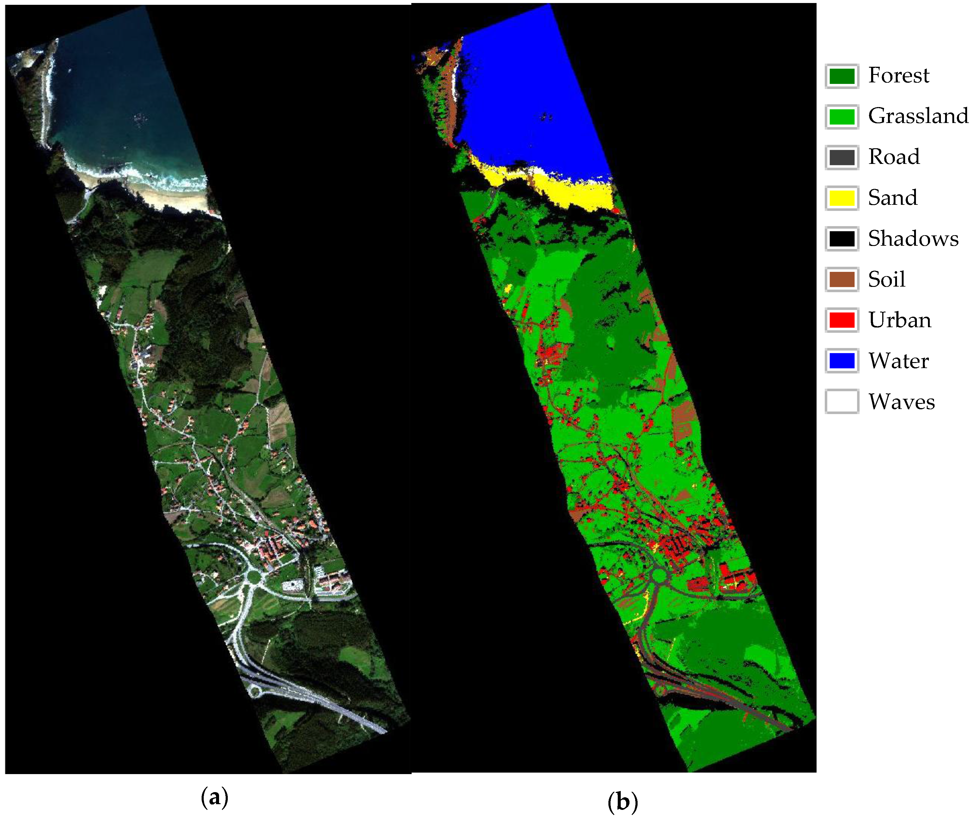
2.1. Study Area and Data Set

The study area is situated in a coastal area of northern Spain, specifically in Reborio (Asturias). The image was acquired and processed in 2011 through the CASI sensor by the Instituto Nacional de Técnica Aeroespacial (INTA). The image was radiometrically corrected and georeferenced, and it has 144 spectral bands and a spatial resolution of 1 m. The classes selected for the classification were forest, meadow, road, shadows, sand, bare soil, urban, water, and waves.

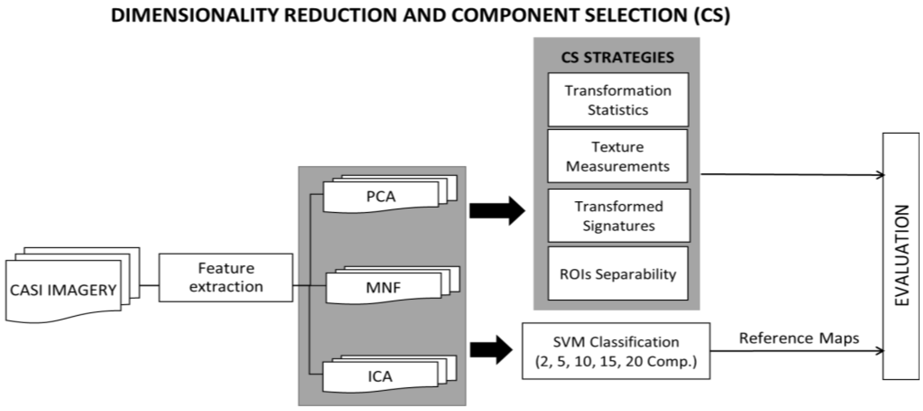
2.2. Dimensionality Reduction Methodology

A preliminary analysis based on three different dimensionality reduction methods—PCA, MNF, and ICA—was performed to determine the number of valuable components containing most of the statistical information. Next, a brief description of them is included.

2.2.1. Dimensionality Reduction Techniques

PCA is often used for the dimensionality reduction of HSI [3,25,26,27,28,29,30]. It is a mathematical orthogonal transformation that changes a set of observations of possibly correlated variables into a set of uncorrelated variables called principal components [31]. PCA retains most of the information of the original data in a low-dimensional space [13]. Conventional PCA faces three main challenges: (1) obtaining a covariance matrix in an extremely large spatial dimension; (2) dealing with the high computational cost required for the analysis of a large dataset; and (3) retaining locally structured elements that appear in a small number of bands for improved discriminant ability when feature bands are globally extracted as principal components [1]. Besides this, PCA equates variance with information and is based on the assumption that the data structure can be described by a multidimensional normal distribution. The performance of PCA depends on the noise characteristics. When noise variance is larger than the signal variance in one band or when the noise is not uniformly distributed between each band, PCA does not guarantee that the amount of information decreases for principal components with a lower ranking [32].

MNF is a noise-adjusted principal component transform that equalizes and estimates the amount of noise in each image band to ensure that the output components are ordered by their information amount [33]. The MNF transform, like PCA, is an eigenvector procedure based on the covariance structure of the noise in the image dataset. MNF is a linear transform consisting of two different steps: (1) computation of the covariance matrix to decorrelate and rescale the noise in the data; and (2) the performance of a standard PCA transform of the decorrelated and rescaled noise data. The goal of the MNF transform is to select components such they maximize the Signal-to-Noise Ratio (SNR), which compares the level of the signal to the level of the background noise rather than the information content [13]. The fact of ordering the components according to the amount of information results in a more reliable identification and elimination of noisy components, and allows for the preservation of components that contain useful information [9,13].

ICA has a wide range of potential applications [32]. Its goal is to decompose a multivariate random measured signal into a linear combination of independent source signals [2]. In contrast with PCA, ICA not only decorrelates second-order statistics but also reduces higher-order statistical dependencies, attempting to make the signals as independent as possible. It is an alternative approach to PCA for dimensionality reduction because it is designed to search for more independent factors that can linearly generate the returns instead of searching for principal components, which allow us to represent the maximum of the return dispersion [5].

2.2.2. Component Selection Strategies

Different strategies were evaluated to select the suitable number of components which contained the most statistical information for each dimensionality reduction method (Figure 1):

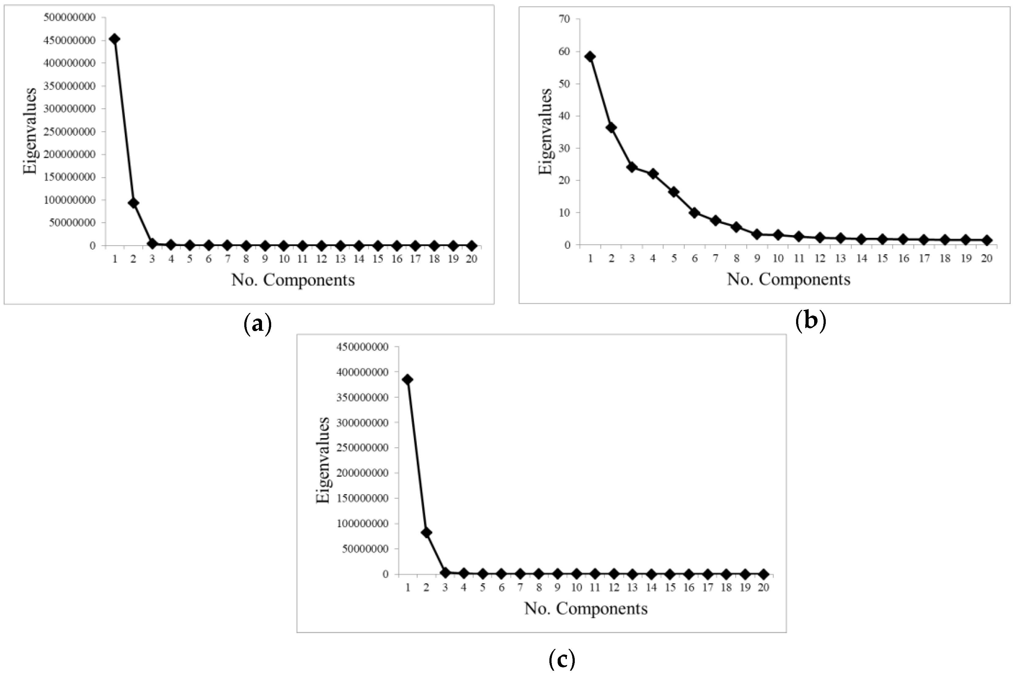
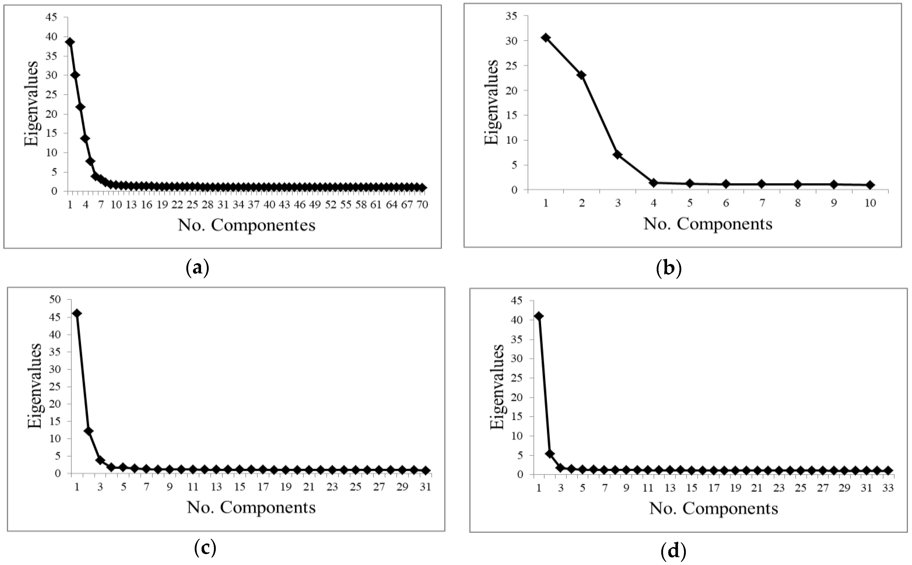
• Transformation statistics: it is the most common method used in the bibliography to select the suitable number of components. The eigenvalues of the obtained components were analyzed [34]. Components with large eigenvalues contain a higher amount of data variance, while components with lower eigenvalues contain less data information and more noise [31].
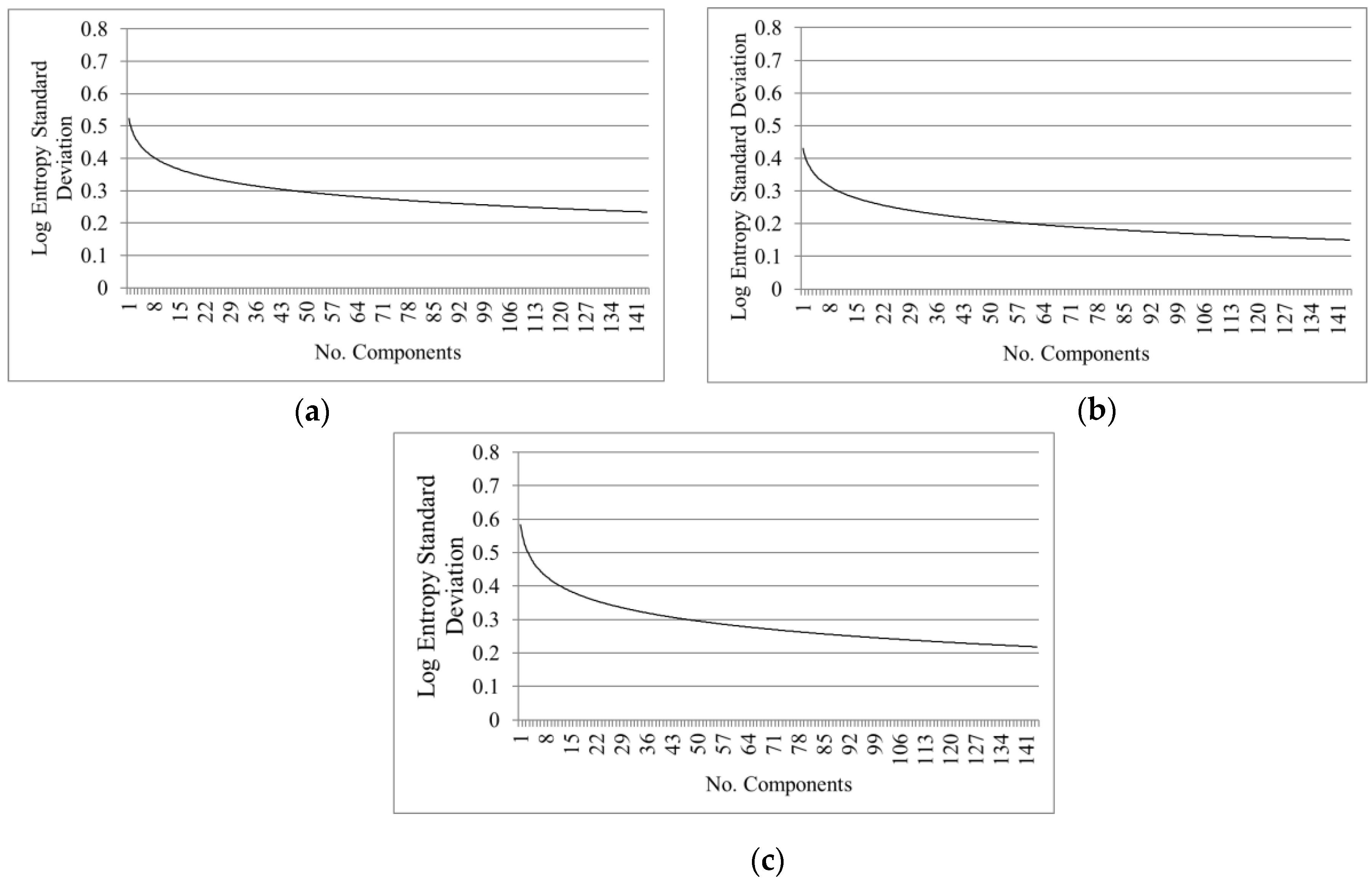
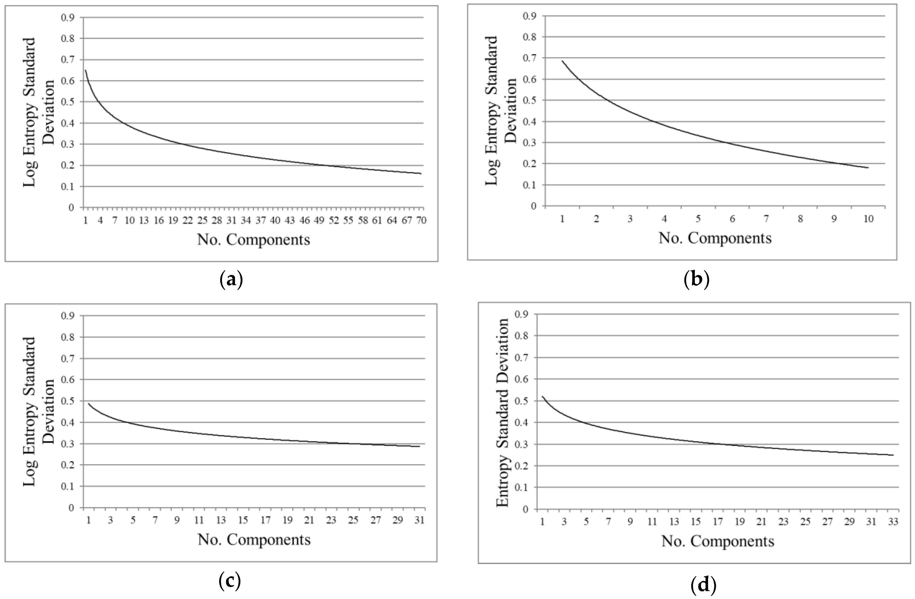
• Texture measurements: texture parameters, as entropy, are simple mathematical representations of image features. These features represent high-level information that can be used to describe the objects in and structure of images [10,35], and in consequence can be applied to select the components providing important information. An entropy first-order texture filter is applied based on a co-occurrence matrix [31]. The Equation (1) from Anys et al. [36] was used to compute the entropy using the pixel values in a kernel centered at the current pixel. Entropy is calculated based on the distribution of the pixel values in the kernel. It measures the disorder of the kernel values, where ${\mathrm{N}}_{\mathrm{g}}$ is the number of distinct grey levels in the image, and $\mathrm{P}\left(\mathrm{i}\right)$ is the probability of each pixel value.

  $$\mathrm{Entropy}=-{\displaystyle \sum }_{\mathrm{i}=0}^{{\mathrm{N}}_{\mathrm{g}}}\mathrm{P}\left(\mathrm{i}\right)\ast \ln \mathrm{P}\left(\mathrm{i}\right)$$

  (1)
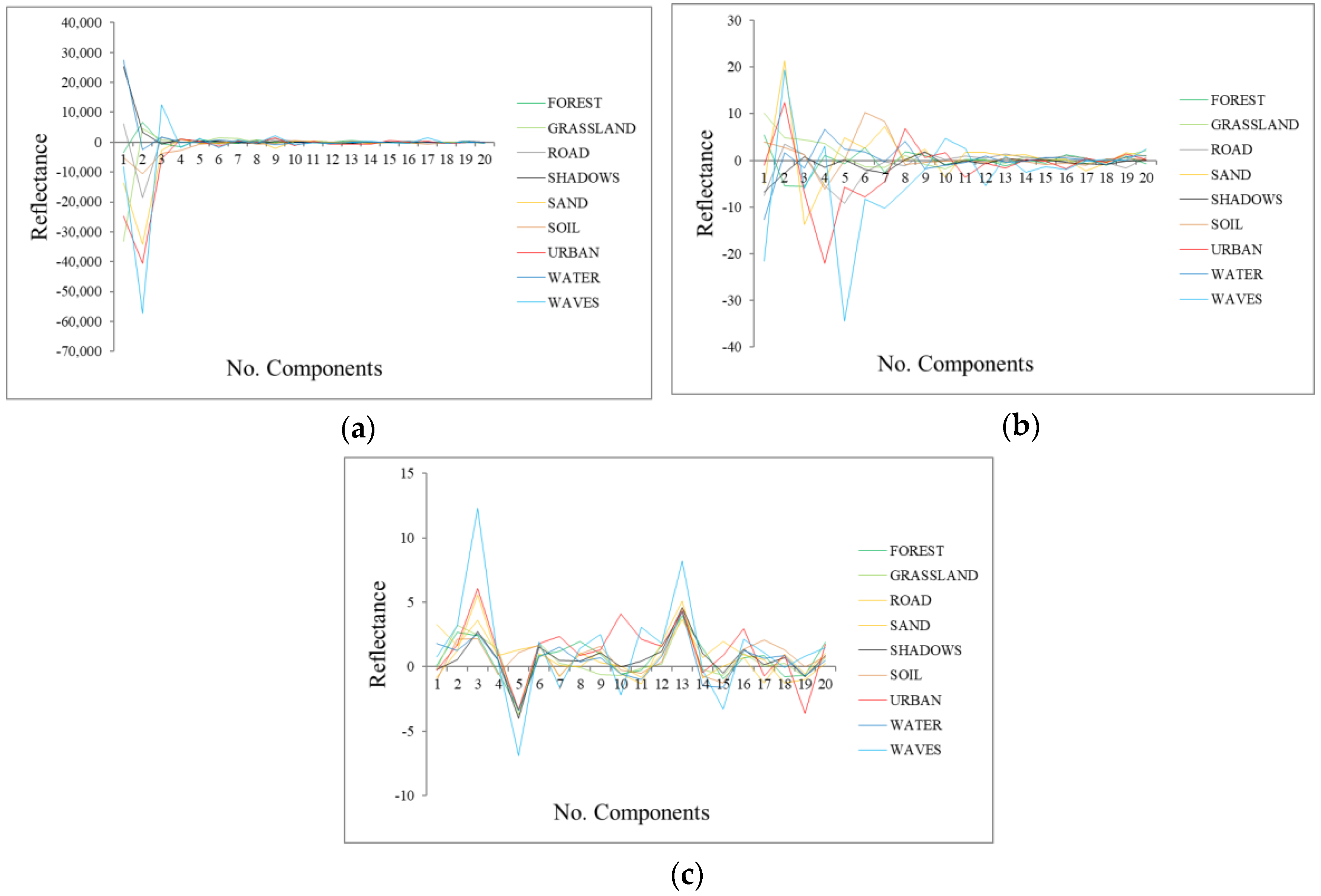
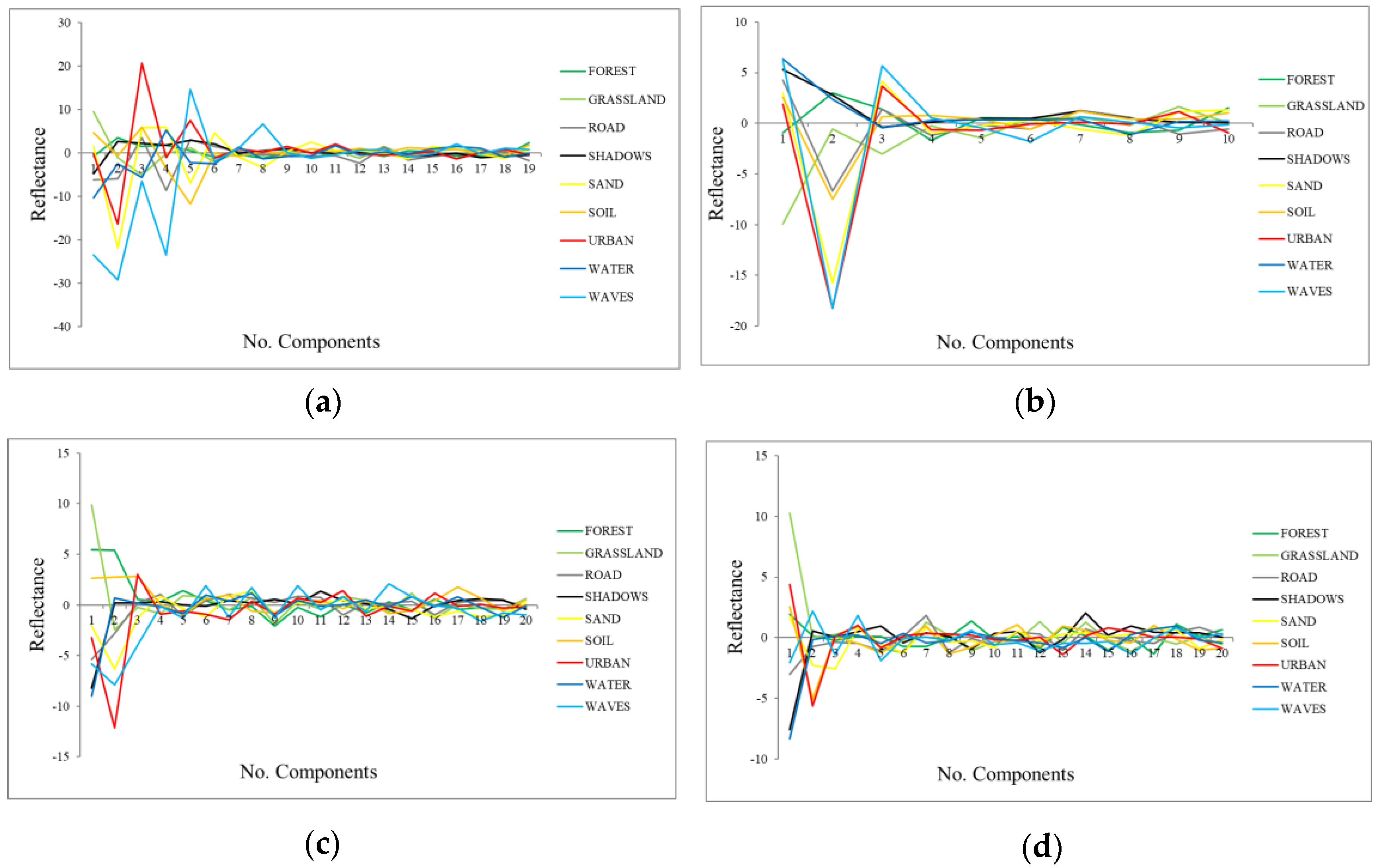
• Signatures of the classes in the transformed space (transformed signatures): the classes considered in the study will have values in the components with information, but they will not be distinguished within each other if the component is mainly noise. Moreover, spatially, in components without noise, objects’ shapes are recognizable, while in noisy components, only a “salt and pepper” effect appears. A visual assessment is used in order to determine from which components the classes cannot be distinguished within each other, being that those components are mainly noise. However, transformed signatures are dependent on the classes determined by each user as well as the type of image.
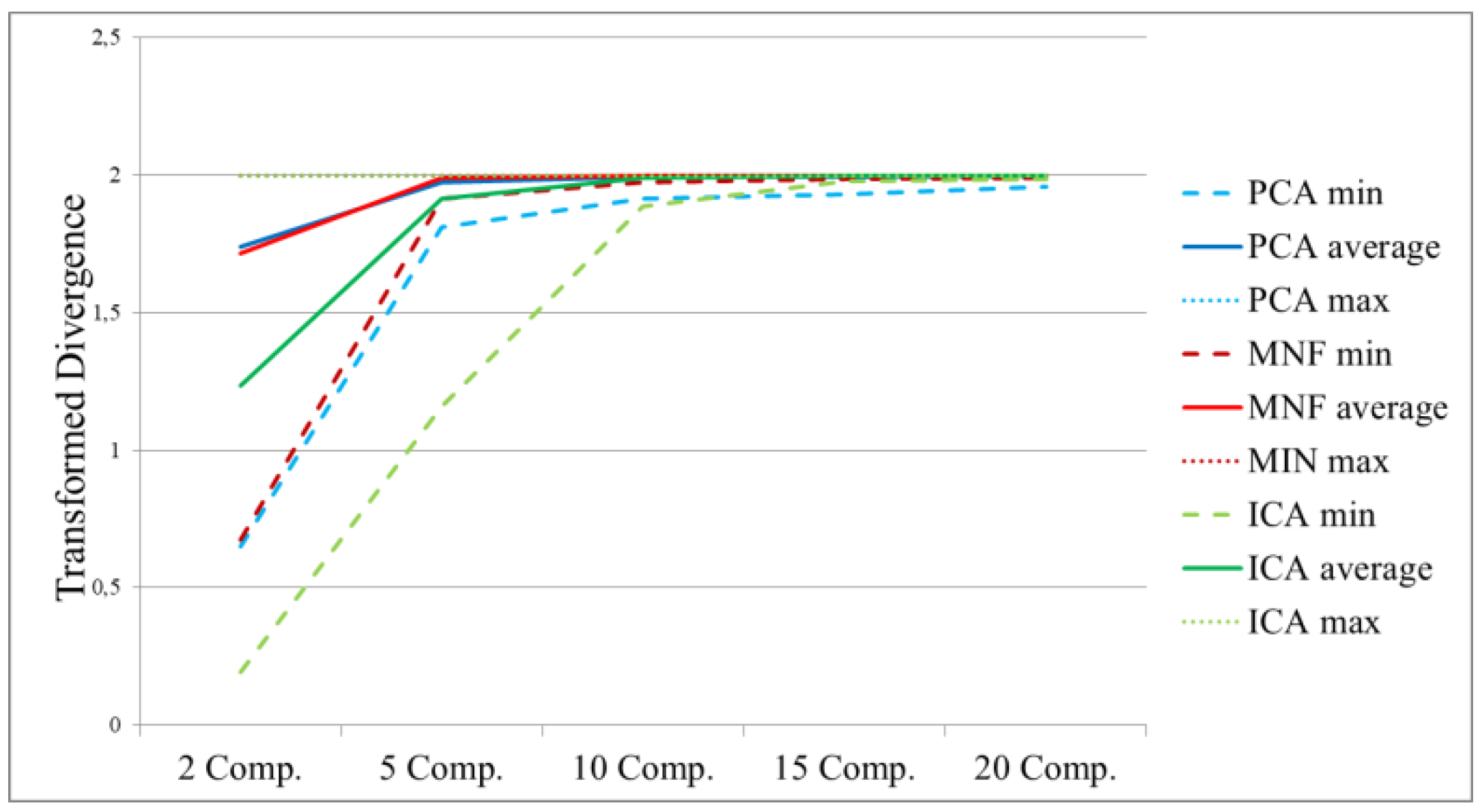
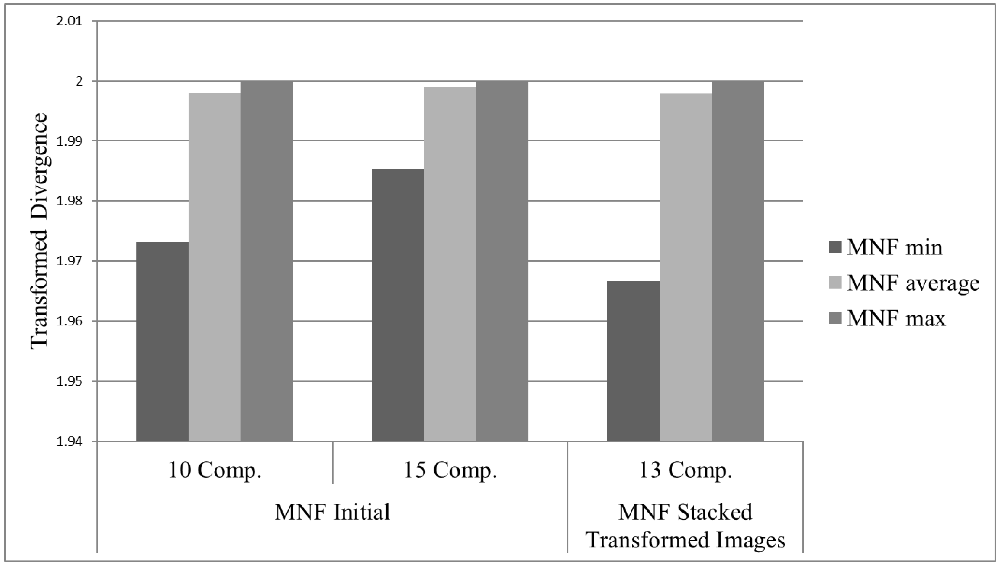
• ROIs separability in the transformed space: during the supervised classification procedure, training and testing regions were selected for each class of interest. The evaluation of the separability in different numbers of components could benefit the selection procedure. This strategy is class-dependent. An ROI’s separability was determined through the Transformed Divergence (TD) measure (2). This separability index exponentially takes into account the mean and the covariance, and its value ranges from 0 to 2 to indicate how well the selected ROI pairs are statistically separable. Values greater than 1.8 indicate that an ROI pair has good separability [31].

  $$\mathrm{TD}=2\left(1-{\mathrm{e}}^{-\frac{\mathrm{D}}{8}}\right)$$

  (2)

Finally, the evaluation was performed using as a reference the accuracy of the classifications carried out for different numbers of components. The method used for the classifications’ validation is known as cross-validation, in which the input data is divided into randomly selected training and testing (ROIs) samples. The testing samples were evaluated against the classified pixels to check if the classifier can properly reproduce the output. The Overall Accuracy (OA), given as a percentage, is obtained from the standardized confusion Error Matrix that compares the thematic map and the rest of the samples selected.

A Support Vector Machine (SVM) algorithm was used in order to evaluate a dimensionality reduction method’s performance. It has been widely used for HSI classification and relies on training data for model optimization [1,3,26]. SVM is one of the most used kernel learning algorithms, which carries out a robust non-linear classification of the image’ pixels using the kernel trick. The idea is to find a separating hyperplane in a higher dimensionality feature space induced by the kernel function while all the computations are done in the original space [3,22]. In other words, it aims to find a hyperplane that makes the average classification error of the training data reach its minimum. As was mentioned, the kernel function is the key factor of the SVM classifier. Typical kernels are the linear, the polymodal, the sigmoid and the radial basis function (RBF) kernel functions [2]. The RBF kernel function, a type of feed-forward Neural Network [26], is selected in the study because it is considered a robust kernel function for remote sensing imagery [37,38,39].

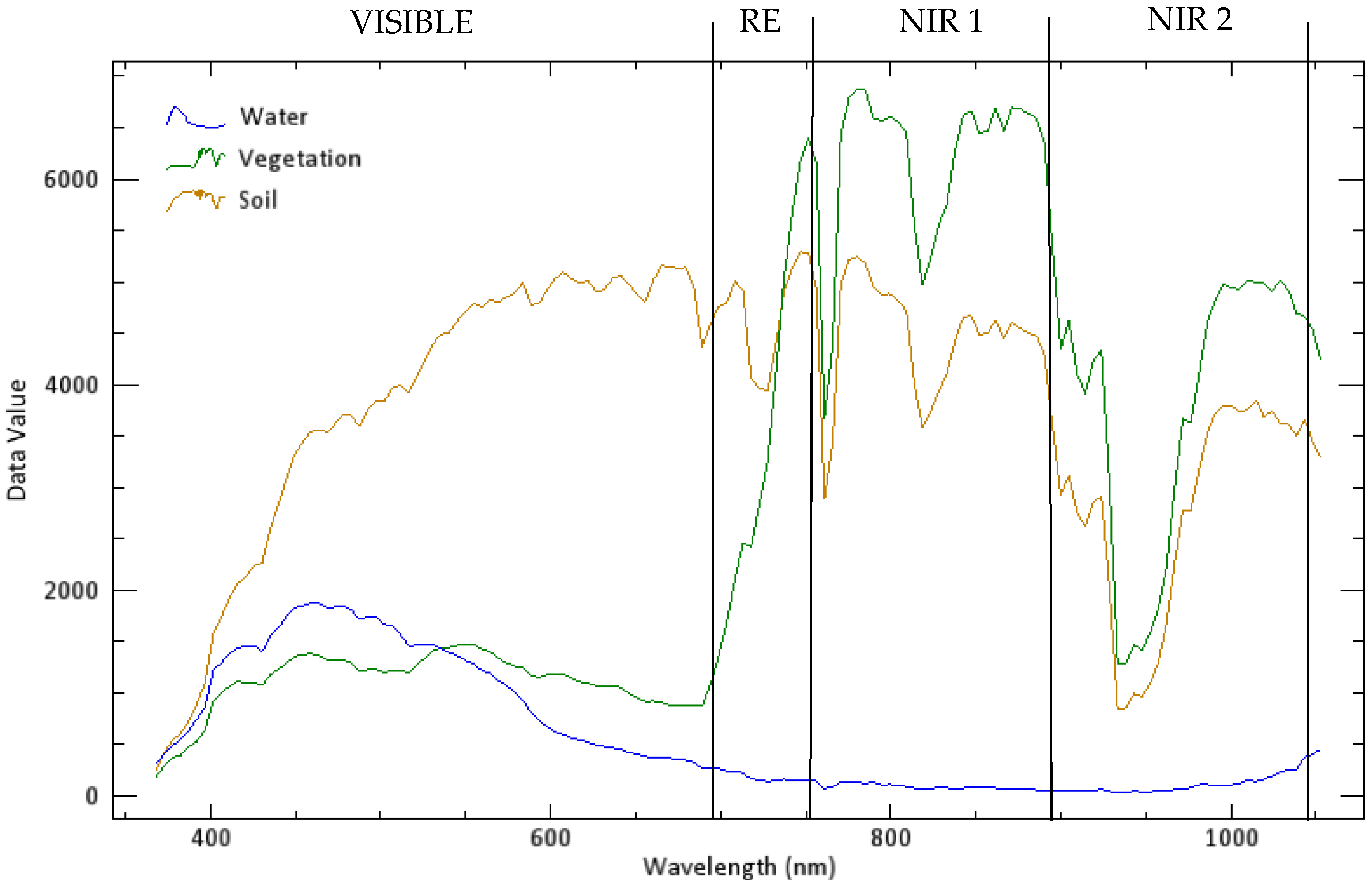
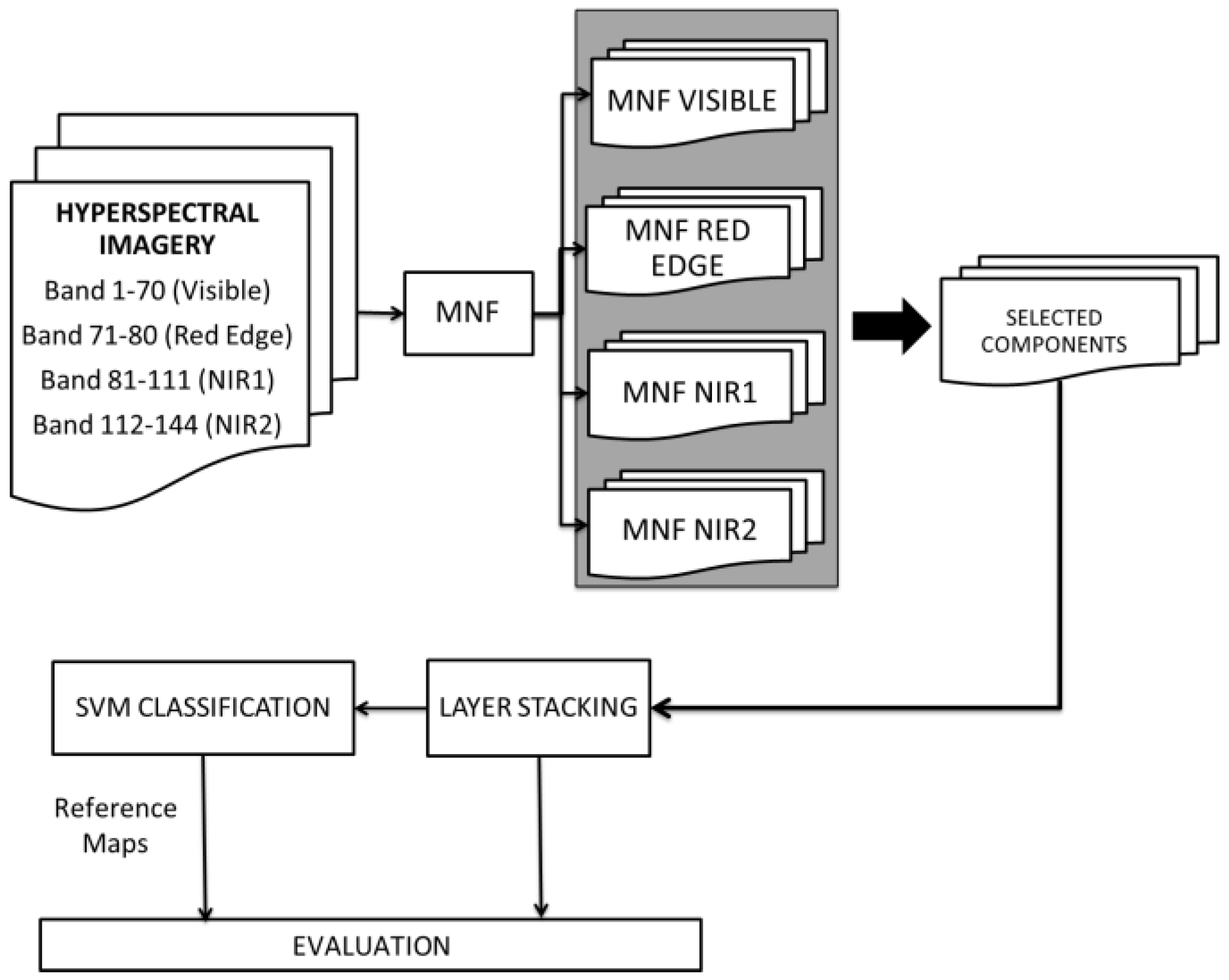
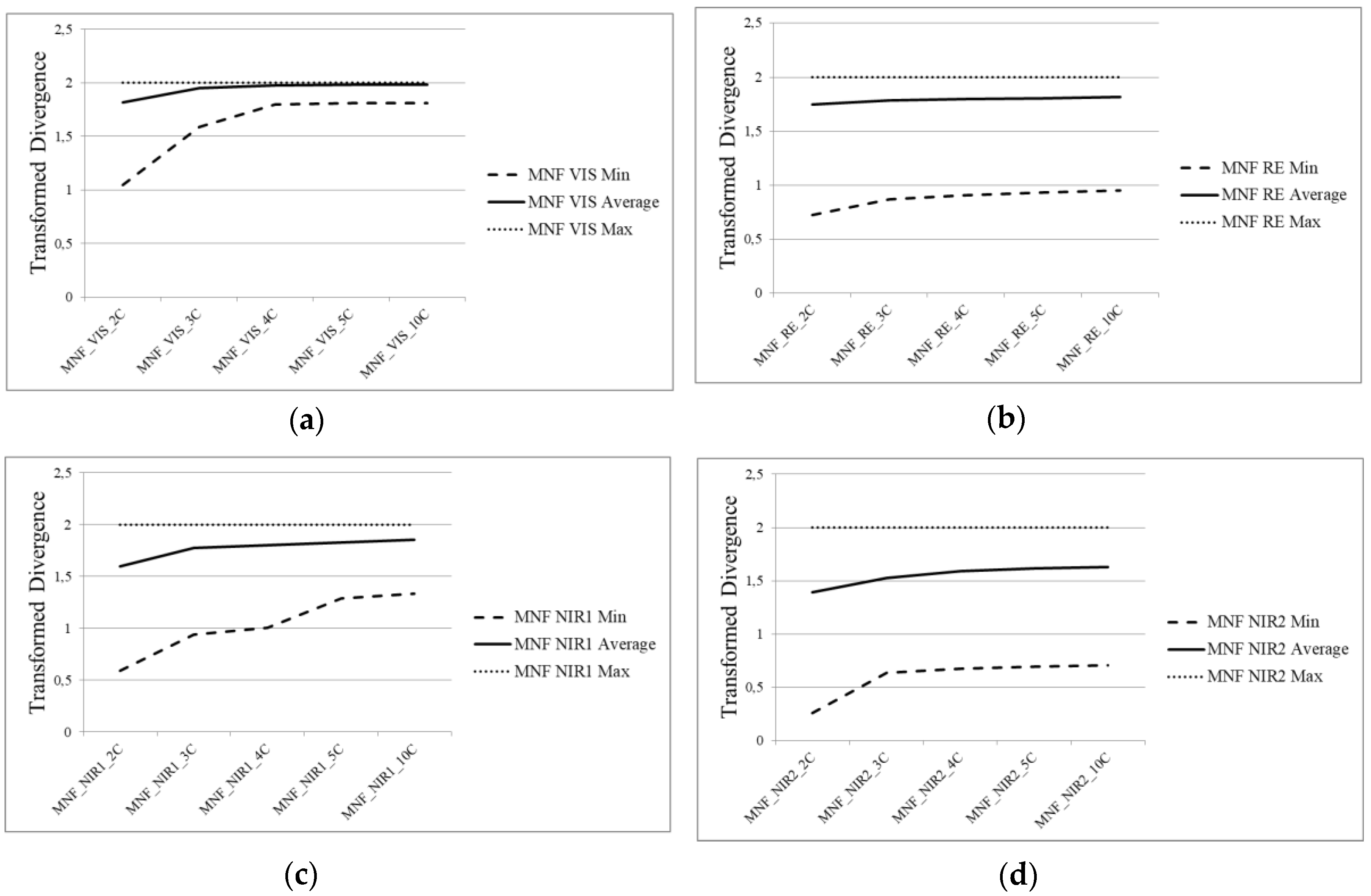
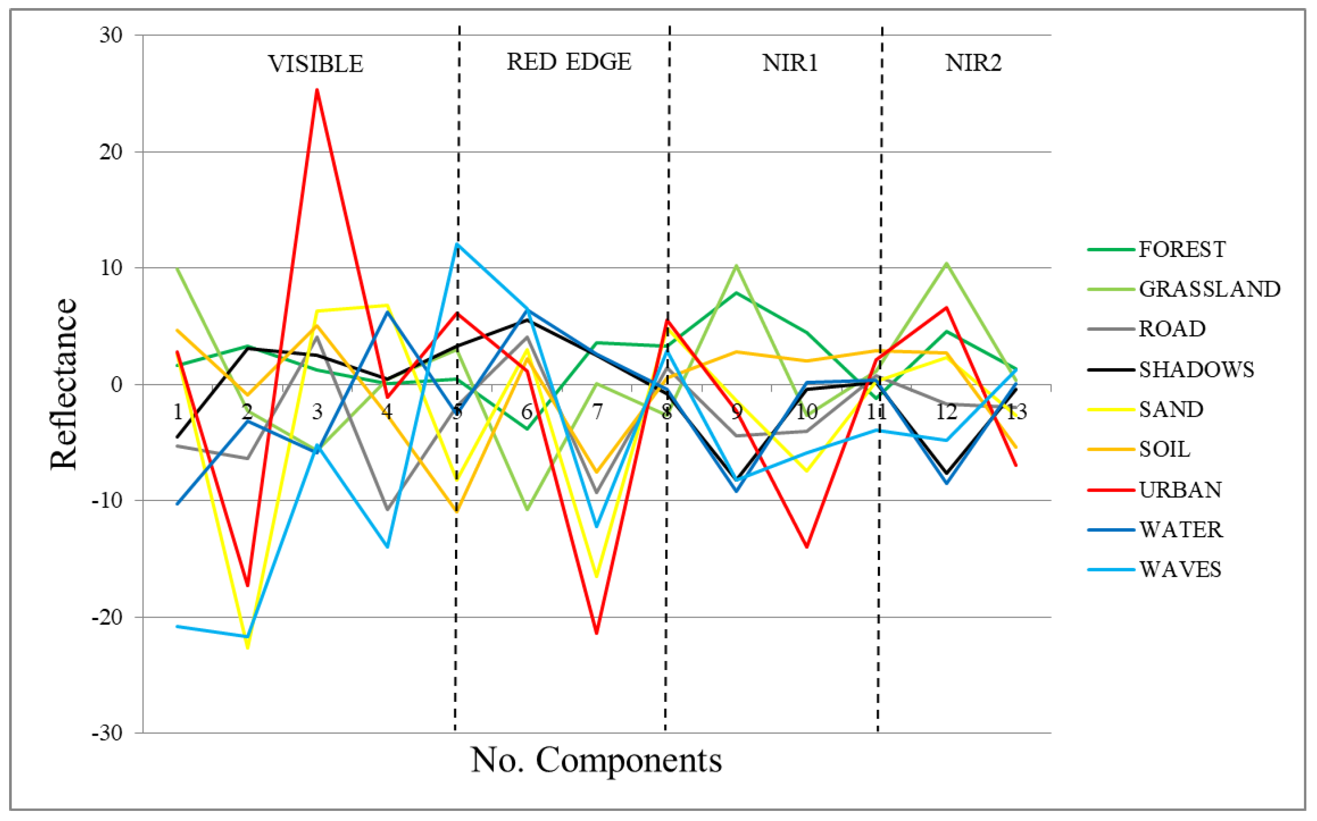
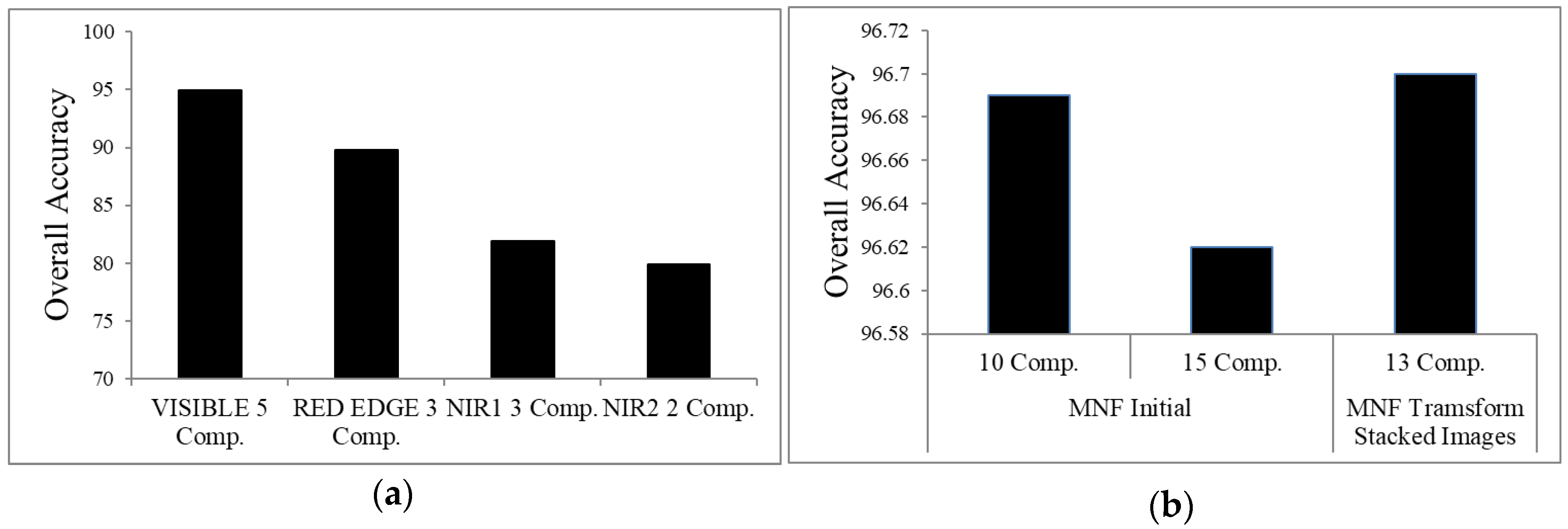
2.2.3. Spectral Division Analysis

Apart from the previous analysis, another study was conducted in order to assess if applying a dimensionality reduction technique independently to different regions of the spectrum (Figure 2) could improve the classification performance in the final transformed space obtained

We call “spectral division” a division where the CASI spectral bands are separated into four groups. The four groups are (1) the Visible region: bands 1 to 70 (368.3–698.7 nm), (2) the Red Edge region: bands 71 to 80 (705.5–751.5 nm), (3) the NIR1 (Near Infrared 1) region: bands 81 to 111 (751.5–895.6 nm), and (4) the NIR2 (Near Infrared 2) region: bands 112 to 144 (899.9–1052.7 nm).

Figure 3 shows the flow diagram of the spectral division analysis as part of the dimensionality reduction process. After the preliminary assessment, the best reduction technique was selected for this analysis (the MNF technique, as will be discussed in Section 3). Once the different spectral regions were selected, a dimensionality reduction transformation was performed independently on each of them. Then, different numbers of components were selected using the component selection strategies described in Section 2.2.2. After selecting the different numbers of components, a layer stacking was carried out for obtaining a transformed space with the selected number of components of each spectral region. Moreover, SVM classifications were performed on the components selected in each region group and in the transformed space obtained from the selected component stacks.

3. Results and Discussion

3.1. Dimensionality Reduction Techniques

This section includes the results obtained from the methodology shown in Figure 1. Section 3.1.1 shows the results obtained from the SVM classification, while Section 3.1.2 shows the results of the different component selection strategies.

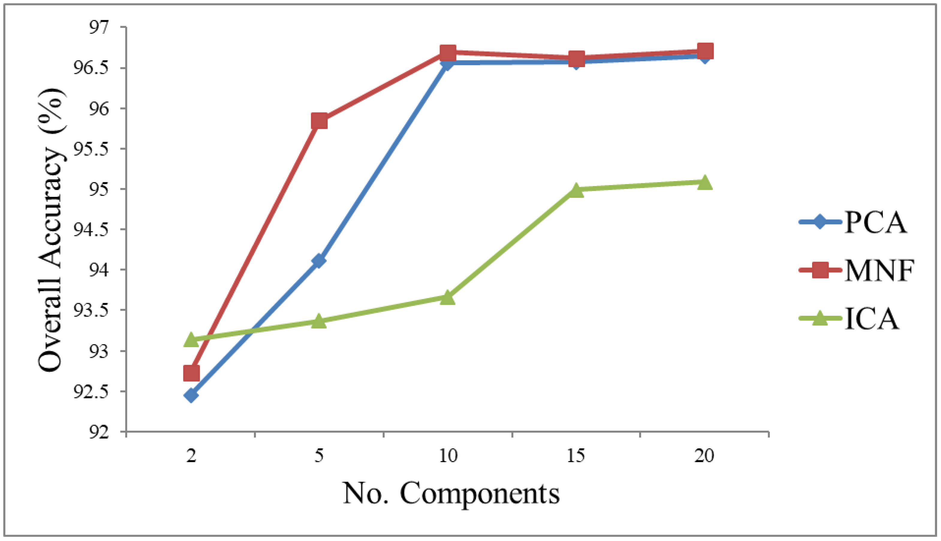
3.1.1. Classification Results for Each Technique

The samples chosen for the classification were taken randomly. Seventy percent of the samples were used for training and 30% for testing. The classes chosen were forest (4797 pixels), meadow (6501 pixels), road (1226 pixels), shadows (2428 pixels), sand (1574 pixels), bare soil (760 pixels), urban (1090 pixels), water (6886 pixels), and waves (141 pixels). The SVM classifier, using the RBF kernel and the appropriate parameters (gamma = 0.1; penalty = 100), was trained with a different number of components from the three dimensionality reduction methods considered. The evaluation was carried out by choosing the 2, 5, 10, 15, and 20 first components after performing the three dimensionality reduction methods (PCA, MNF, and ICA). Due to the noise of the last components chosen, it is expected that the accuracy results should decrease when adding more components.

Figure 4 shows the OA for each method and for a given number of components. It can be observed that MNF achieves the highest accuracy. The OA in the PCA transformed space and the OA in the MNF transformed space are stabilized using 10 components, whereas ICA needs at least 15 components to stabilize the OA, but with a lower OA than the PCA transformed space and the MNF transformed space. Figure 5 shows the thematic map obtained from the best SVM classification, which is uses the MNF transformed space with 10 components (OA: 96.68%).

This information about the minimum number of components required to achieve the best performance will be the reference information to assess the different component selection methods.

3.1.2. Results for the Component Selection Strategies

As indicated in Figure 1, four component selection strategies were analyzed.

In this context, the first strategy is based on the calculation of eigenvalues. Figure 6 shows the eigenvalues obtained after carrying out PCA, MNF, and ICA transforms. Eigenvalues with higher values provide more information than eigenvalues with values close to zero, which contain mainly noise. Thus, visually, only 2 components concentrate most of the information for PCA, 10 for MNF, and 2 for ICA.

The texture measurement of each component was extracted using the entropy. From the experiments, it can be observed that the mean of the entropy does not show an appropriate pattern for component selection but the standard deviation does (Figure 7). In this case, the components with the highest information obtain higher standard deviation values (the figure is shown in a logarithmic scale in order to offer a better visualization). It is observed that, around the 10th component, the logarithmic curve changes its slope in PCA and MNF, while in ICA it changes around the 15th component.

Figure 8 shows the transformed signatures of the different classes. Since the different dimensionality reduction techniques give different results, the scale is different. Only components 1 to 20 are presented to facilitate the observation of the classes difference in the first components. Figure 8 shows how signatures in the transformed space allow us to discriminate some classes from others, but only for the first components. This result is consistent with Figure 9, where the separability measures of each class are shown as a function of the number of components. The greatest separability of the ROIs is from the 10 components for PCA and MNF and the 15 for ICA, which is in agreement with the results shown in Figure 4.

Table 1. Results comparison of SVM classification and strategies to determine components (comp.).

		PCA	MNF	ICA
EVALUATION	SVM Classification	Good (10 comp.)	Best (10 comp.)	Medium (15 comp.)
COMPONENT SELECTION STRATEGIES	Eigenvalues	Wrong (2 comp.)	Good (9 comp.)	Wrong (2 comp.)
	Entropy	Good (10 comp.)	Good (10 comp.)	Good (15 comp.)
	Signatures of the classes	Good (9 comp.)	Good (10 comp.)	Medium (11 comp.)
	ROIs separability	Good (10 comp.)	Good (10 comp.)	Good (15 comp.)

shows a qualitative assessment, summarizing the quantitative results for determining the component selection strategy that most closely matches with the results obtained in the classifications. ‘Good’ means that the strategy achieves a good agreement with the number of components determined by the SVM algorithm, ‘Wrong’ means that the number of bands selected by the strategy does not match with the SVM algorithm’s results. Thus, we can observe which measurement may be the most adequate to determine the number of components to be used for the dimensionality reduction of HSI.

From the results summarized in Table 1, as indicated in the first row, it is observed that MNF and PCA are more reliable techniques, because they do not need a great number of components in the classification, as is the case with the ICA technique. Moreover, PCA and MNF obtained similar OA values, being slightly better those of MNF. On the other hand, the best classification results regarding the different numbers of components (PCA 10 comp., MNF 10 comp., and ICA 15 comp.) are taken as a reference to determine the suitable strategy for selecting an adequate number of components. Thus, as indicated, if the number of components determined by a particular strategy is equal or very close to the number of components for which the best SVM classification result is attained, the strategy is labeled as ‘Good’. Hence, the eigenvalues with information obtained for PCA and ICA (two components in both techniques) do not match with the result of the classification. On the other hand, the remaining different dimensionality reduction techniques got a good determination of components using the entropy measurement (PCA and MNF the logarithmic curve changes around the 10th component while it changes around the 15th component for the ICA technique). Finally, it can be observed that the entropy, transformed signatures of the classes, and the ROIs separability in the transformed space match with the results obtained for the classification with the SVM algorithm, and are suitable methods for selecting an adequate number of components with more statistical information.

3.2. Spectral Division Analysis Results

From the results shown in Section 3.1, MNF is the most suitable dimensionality reduction technique. Thus, it was chosen for the second part of the study, where the HSI was divided into groups according to different regions of the electromagnetic spectrum (the Visible, Red Edge, NIR1, and NIR2 regions). In this part of the study, MNF was applied separately to the each of them.

Figure 10 shows the eigenvalues for each spectral region. Figure 11 and Figure 12 show the entropy’s standard deviation and the transformed signatures of the classes, respectively. Figure 11 shows the ROIs separability results when taking different numbers of components in the transformed space.

Table 2. Selected components of each region regarding the Eigenvalues, Entropy, Transformed signatures of classes, and ROIs separability in the transformed space.

REGIONS	EIGENVALUES	ENTROPY	SIGNATURES OF CLASSES	ROIS SEPARABILITY
Visible	5 comp.	5 comp.	5 comp.	4 comp.
Red Edge	3 comp.	3 comp.	3 comp.	3 comp.
NIR1	3 comp.	3 comp.	3 comp.	3 comp.
NIR2	2 comp.	3 comp.	2 comp.	3 comp.

shows the components selected for each region regarding the eigenvalue, entropy, transformed signatures of the classes, and ROIs separability approaches.

Regarding the eigenvalues strategy, the numbers of components selected for each region are: five for the Visible region, three components for the Red Edge region and for the NIR1 region, and finally only two components have information for the NIR2 region, (Figure 10 and Table 2). Concerning the entropy’s standard deviation, the components with the highest information obtain higher standard deviation values, being five in the Visible region, three in the Red Edge and NIR1 regions, and three in the NIR2 region (Figure 12, Table 2). Observing the transformed signatures of the classes, five components are selected for the Visible region, again three components for the Red Edge and NIR1 regions, and two components are selected for the NIR2 region (Figure 13, Table 2). Finally, in Figure 11, the ROIs separability results are stabilized using four components in the Visible region, and three components for Red Edge, NIR1, and NIR2 spectral regions (Table 2).

As observed in Table 2, there are some disagreements in the number of components for the Visible and the NIR2 regions, where finally five and two components were selected, respectively. Thus, we decided to create a stacked transformed space with five components for the Visible region, three for the Red Edge and NIR1 regions, and two for the NIR2 region.

Once the MNF stacked transformed space with 13 components was generated, the ROIs separability of the components selected in each spectral division group, as well as in the stacked transformed space, was computed (Figure 14). Moreover, the signatures in the stacked transformed space were obtained (Figure 15). Finally, SVM classifier was applied to the components selected in each spectral division group and in the stacked transformed space (Figure 16). Then, the SVM accuracies were compared with the SVM classifications obtained in Section 3.1 in order to evaluate not only which methodology is more suitable for obtaining an accurate thematic map but also to assess the influence of using the appropriate components in the classification process.

Figure 14 shows the ROIs separability results from the MNF initial transformation using 10 and 15 components and in the stacked transformed space with 13 components. The minimum value for every transformed space is above 1.9. However, the minimum value in the stacked transformed space is a bit lower than in the original MNF transformations.

The transformed signatures of the classes in the stacked MNF transformed space (Figure 15) reveal, as well, how the visible region discriminates them slightly better, as is the case with the ROIs separability (Figure 11a).

It is again observed, in Figure 16a, how the Visible region obtains a better OA. Regarding the classification accuracy in the MNF transformed spaces, Figure 16b also shows the OA of the SVM classification applied in the MNF initial transformation using 10 and 15 components (see Figure 4), in order to compare with this second approach. SVM classification applied in the stacked MNF transformed space with 13 components obtains the highest accuracy (96.7%), being a bit higher than the original MNF transformation with 10 components (96.69%).

4. Conclusions

The objectives of this study were to carry out a comparative evaluation of classical dimensionality reduction techniques (PCA, MNF, and ICA) in HSI and to assess different strategies for selecting the most suitable number of components. At the same time, we proposed to carry out a dimensionality reduction approach considering a spectral division of the HSI in order to analyze if the number of components selected was more suitable for generating a final thematic map.

In the first part of the study, according to the SVM classification results, MNF was the most suitable dimensionality reduction technique. Regarding the component selection strategies, entropy measurement, transformed signatures of the classes, and ROIs separability strategies are more appropriate for the components’ selection. However, the transformed signatures of the classes and ROIs separability strategies need a manual ROIs selection for each class. In contrast, it was demonstrated that eigenvalues are not the most appropriated method to select a suitable number of components containing most of the statistical information.

On the other hand, the second part of the study proposed a spectral division of the HSI, and then performed an MNF transformation independently on the different regions of the electromagnetic spectrum. Once this MNF transformation was carried out, the components with more information were selected according to the different strategies. It can be observed that using this spectral division approach, when comparing it with the traditional MNF transformation, only slightly improves the components’ selection.

Therefore, after the evaluation, the standard deviation values of the entropy are proposed to determine the appropriate number of components. However, if a supervised classification is carried out, in which the classes and the corresponding ROIs are determined, the transformed signatures of each class as well as the ROIs separability values, in the transformed space, are a good choice. In this way, the selection of components would be adjusted to each user and each classification problem.

A more comprehensive study should be carried out to evaluate if this method would be recommended as a component selection strategy. In consequence, this study is currently being performed using different types of HSI, since these results could be influenced by the imagery considered.

References

1. Ren, J.; Zabalza, J.; Marshall, S.; Zheng, J. Effective feature extraction and data reduction in remote sensing using hyperspectral imaging. IEEE Signal Process. Mag. 2014, 31, 149–154. [Google Scholar] [CrossRef]
2. Li, C.; Yin, J.; Zhao, J. Using improved ICA method for hyperspectral data classification. Arabian J. Sci. Eng. 2014, 39, 181–189. [Google Scholar] [CrossRef]
3. Benediktsson, J.A.; Ghamisi, P. Spectral-Spatial Classification of Hyperspectral Remote Sensing Images; Artech House: Boston, MA, USA, 2015. [Google Scholar]
4. Ballanti, L.; Blesius, L.; Hines, E.; Kruse, B. Tree species classification using hyperspectral imagery: A comparison of two classifiers. Remote Sens. 2016, 8, 445. [Google Scholar] [CrossRef]
5. Villa, A.; Chanussot, J.; Jutten, C.; Benediktsson, J.A.; Moussaoui, S. On the use of ICA for hyperspectral image analysis. In Proceedings of the IEEE International Geoscience and Remote Sensing Symposium (IGARSS), Cape Town, South Africa, 12–17 July 2009; Volume 4, pp. 97–100. [Google Scholar]
6. Melgani, F.; Bruzzone, L. Classification of hyperspectral remote sensing images with support vector machines. IEEE Trans. Geosci. Remote Sens. 2004, 42, 1778–1790. [Google Scholar] [CrossRef]
7. Hughes, G. On the mean accuracy of statistical pattern recognizers. IEEE Trans. Inf. Theory 1968, 14, 55–63. [Google Scholar] [CrossRef]
8. Ghamisi, P.; Benediktsson, J.A.; Phinn, S. Land-cover classification using both hyperspectral and Lidar data. Int. J. Image Data Fusion 2015, 6, 189–215. [Google Scholar] [CrossRef]
9. Fassnacht, F.E.; Neumann, C.; Förster, M.; Buddenbaum, H.; Ghosh, A.; Clasen, A.; Joshi, P.K.; Koch, B. Comparison of feature reduction algorithms for classifying tree species with hyperspectral data on three central European test sites. IEEE J. Sel. Top. Appl. Earth Obs. Remote Sens. 2014, 7, 2547–2561. [Google Scholar] [CrossRef]
10. Ibrahim, R.W.; Moghaddasi, Z.; Jalab, H.A.; Noor, R.M. Fractional differential texture descriptors based on the Machado entropy for image splicing detection. Entropy 2015, 17, 4775–4785. [Google Scholar] [CrossRef]
11. Licciardi, G.A.; Frate, F. In A comparison of feature extraction methodologies applied on hyperspectral data. In Proceedings of the 2010 Hyperspectral Workshop, Frascati, Italy, 17–19 March 2010; pp. 17–19. [Google Scholar]
12. Wang, L.; Zhao, C. Hyperspectral Image Processing; Springer: Berlin, German, 2016. [Google Scholar]
13. Luo, G.; Chen, G.; Tian, L.; Qin, K.; Qian, S.-E. Minimum noise fraction versus principal component analysis as a preprocessing step for hyperspectral imagery denoising. Can. J. Remote Sens. 2016, 42, 106–116. [Google Scholar] [CrossRef]
14. Chang, C.-I.; Du, Q.; Sun, T.-L.; Althouse, M.L. A joint band prioritization and band-decorrelation approach to band selection for hyperspectral image classification. IEEE Trans. Geosci. Remote Sens. 1999, 37, 2631–2641. [Google Scholar] [CrossRef]
15. Cheriyadat, A.; Bruce, L.M. Why principal component analysis is not an appropriate feature extraction method for hyperspectral data. In Proceedings of the IEEE International Geoscience and Remote Sensing Symposium, IGARSS, Toulouse, France, 21–25 July 2003; pp. 3420–3422. [Google Scholar]
16. Du, H.; Qi, H.; Wang, X.; Ramanath, R.; Snyder, W.E. Band selection using independent component analysis for hyperspectral image processing. In Proceedings of the IEEE Applied Imagery Pattern Recognition Workshop, Washington, DC, USA, 15–17 October 2003; Volume 32, pp. 93–98. [Google Scholar]
17. Lennon, M.; Mercier, G.; Mouchot, M.; Hubert-Moy, L. Independent component analysis as a tool for the dimensionality reduction and the representation of hyperspectral images. In Proceedings of the IEEE International Geoscience and Remote Sensing Symposium (IGARSS), Sydney, Australia, 9–13 July 2001; pp. 2893–2895. [Google Scholar]
18. Wang, J.; Chang, C.-I. Independent component analysis-based dimensionality reduction with applications in hyperspectral image analysis. IEEE Trans. Geosci. Remote Sens. 2006, 44, 1586–1600. [Google Scholar] [CrossRef]
19. Liao, W.; Vancoillie, F.; Devriendt, F.; Gautama, S.; Pizurica, A.; Philips, W. Fusion of pixel-based and object-based features for classification of urban hyperspectral remote sensing data. In Proceedings of the 5th International Conference on Geographic Object-Based Image Analysis (GEOBIA), Thessaloniki, Greece, 21–24 May 2014; pp. 179–184. [Google Scholar]
20. Mücher, C.A.; Kooistra, L.; Vermeulen, M.; Borre, J.V.; Haest, B.; Haveman, R. Quantifying structure of natura 2000 heathland habitats using spectral mixture analysis and segmentation techniques on hyperspectral imagery. Ecol. Indic. 2013, 33, 71–81. [Google Scholar] [CrossRef]
21. Cortes, C.; Vapnik, V. Support vector machine. Mach. Learn. 1995, 20, 273–297. [Google Scholar] [CrossRef]
22. Mountrakis, G.; Im, J.; Ogole, C. Support vector machines in remote sensing: A review. ISPRS J. Photogramm. Remote Sens. 2011, 66, 247–259. [Google Scholar] [CrossRef]
23. Rojas, M.; Dópido, I.; Plaza, A.; Gamba, P. Comparison of support vector machine-based processing chains for hyperspectral image classification. Proc. SPIE 2010, 78100B. [Google Scholar] [CrossRef]
24. Denghui, Z.; Le, Y. Support vector machine based classification for hyperspectral remote sensing images after minimum noise fraction rotation transformation. In Proceedings of the IEEE International Conference Internet Computing & Information Services (ICICIS), Hong Kong, China, 17–18 September 2011; pp. 32–135. [Google Scholar]
25. Rodarmel, C.; Shan, J. Principal component analysis for hyperspectral image classification. Surv. Land Inf. Sci. 2002, 62, 115. [Google Scholar]
26. Chandrashekar, G.; Sahin, F. A survey on feature selection methods. Comput. Electr. Eng. 2014, 40, 16–28. [Google Scholar] [CrossRef]
27. Wiersma, D.J.; Landgrebe, D.A. Analytical design of multispectral sensors. IEEE Trans. Geosci. Remote Sens. 1980, GE-18, 180–189. [Google Scholar] [CrossRef]
28. Drumetz, L.; Veganzones, M.A.; Gómez, R.M.; Tochon, G.; Dalla Mura, M.; Licciardi, G.A.; Jutten, C.; Chanussot, J. Hyperspectral local intrinsic dimensionality. IEEE Trans. Geosci. Remote Sens. 2016, 54, 4063–4078. [Google Scholar] [CrossRef] [Green Version]
29. Kaewpijit, S.; Le-Moige, J.; El-Ghazawi, T. Hyperspectral Imagery Dimension Reduction Using Principal Component Analysis on the HIVE. In Proceedings of the Science Data Processing Workshop, Greenbelt, MD, USA, 26–28 February 2002. [Google Scholar]
30. Vidal, M.; Amigo, J.M. Pre-processing of hyperspectral images. Essential steps before image analysis. Chemom. Intell. Lab. Syst. 2012, 117, 138–148. [Google Scholar] [CrossRef]
31. Richards, J.A. Remote Sensing Digital Image Analysis; Springer: Berlin, Germany, 1999; Volume 3. [Google Scholar]
32. Hyvärinen, A.; Oja, E. Independent component analysis: Algorithms and applications. Neural Netw. 2000, 13, 411–430. [Google Scholar] [CrossRef]
33. Green, A.A.; Berman, M.; Switzer, P.; Craig, M.D. A transformation for ordering multispectral data in terms of image quality with implications for noise removal. IEEE Trans. Geosci. Remote Sens. 1988, 26, 65–74. [Google Scholar] [CrossRef]
34. Francis, J.G. The QR transformation—Part 2. Comput. J. 1962, 4, 332–345. [Google Scholar] [CrossRef]
35. Padmanaban, R.; Bhowmik, A.K.; Cabral, P.; Zamyatin, A.; Almegdadi, O.; Wang, S. Modelling urban sprawl using remotely sensed data: A case study of Chennai city, Tamilnadu. Entropy 2017, 19, 163. [Google Scholar] [CrossRef]
36. Anys, H.; Bannari, A.; He, D.; Morin, D. Texture analysis for the mapping of urban areas using airborne MEIS-II images. In Proceedings of the First International Airborne Remote Sensing Conference and Exhibition, Strasbourg, France, 12–15 September 1994; Environmental Research Institute of Michigan: Ann Arbor, MI, USA, 1994; pp. 231–245. [Google Scholar]
37. Huang, X.; Zhang, L. An SVM ensemble approach combining spectral, structural, and semantic features for the classification of high-resolution remotely sensed imagery. IEEE Trans. Geosci. Remote Sens. 2013, 51, 257–272. [Google Scholar] [CrossRef]
38. Pal, M.; Mather, P.M. Assessment of the effectiveness of support vector machines for hyperspectral data. Future Gener. Comput. Syst. 2004, 20, 1215–1225. [Google Scholar] [CrossRef]
39. Braun, A.C.; Weidner, U.; Hinz, S. Support vector machines for vegetation classification—A revision. Photogramm. Fernerkund. Geoinf. 2010, 2010, 273–281. [Google Scholar] [CrossRef]
Figure 1. Flow diagram of the methodology proposed for evaluation of component selection strategies. CASI: Compact Airborne Spectrographic Imager; PCA: Principal Component Analysis; MNF: Minimum Noise Factor; ICA: Independent Component Analysis; ROI: region of interest; SVM: Support Vector Machine.
Entropy 19 00666 g001
Figure 2. Representative spectral reflectance curves for several common Earth surface materials over the visible light to the reflected infrared spectral range (VISIBLE: Visible region; RE: Red Edge region; NIR 1: Near Infrared 1 Region; NIR 2: Near Infrared 2 Region).
Entropy 19 00666 g002
Figure 3. Diagram flow of the spectral division analysis.
Entropy 19 00666 g003
Figure 4. The Support Vector Machine (SVM) Algorithm’s Overall Accuracy for 2, 5, 10, 15, and 20 components.
Entropy 19 00666 g004
Figure 5. (a) RGB (Red Green Blue) color composite; (b) SVM classification map obtained from the 10 first components of the Minimum Noise Fraction (MNF) transform.
Entropy 19 00666 g005
Figure 6. Eigenvalues of the first 20 components: (a) Principal Component Analysis (PCA); (b) MNF; and (c) Independent Component Analysis (ICA).
Entropy 19 00666 g006
Figure 7. Entropy standard deviation: (a) PCA; (b) MNF; and (c) ICA.
Entropy 19 00666 g007
Figure 8. Transformed signatures of each class in: (a) PCA; (b) MNF; and (c) ICA.
Entropy 19 00666 g008
Figure 9. ROIs separability in the transformed space of PCA, MNF, and ICA. Comp: components.
Entropy 19 00666 g009
Figure 10. Eigenvalues obtained from the MNF transformation: (a) Visible region; (b) Red Edge region; (c) NIR 1 region; and (d) NIR 2 region.
Entropy 19 00666 g010
Figure 11. ROIs separability in the transformed space of: (a) the Visible region (MNF_VIS_XC, X: no. of components); (b) the Red Edge region (MNF_RE_XC); (c) the NIR1 region (MNF_NIR1_XC); and (d) the NIR2 region (MNF_NIR2_XC).
Entropy 19 00666 g011
Figure 12. Entropy Standard Deviation: (a) Visible region; (b) Red Edge region; (c) NIR1 region; and (d) NIR2 region.
Entropy 19 00666 g012
Figure 13. Transformed signatures of each class in: (a) the Visible region; (b) the Red Edge region; (c) the NIR1 region; and (d) the NIR2 region.
Entropy 19 00666 g013
Figure 14. ROIs separability of the MNF transformed space of the initial transformation (spectral division not applied) using 10 and 15 components and from the stacked transformed space (13 comp.).
Entropy 19 00666 g014
Figure 15. Transformed signatures of the classes in the stacked MNF transformed space: 13 comp.
Entropy 19 00666 g015
Figure 16. Overall Accuracy (%) of SVM classification of MNF transformed space for: (a) the components selected in each spectral region; and (b) MNF initial transformation (spectral division not applied) using 10 and 15 components and from the stacked transformed space (13 comp.).
Entropy 19 00666 g016