Quantum Minimum Distance Classifier

Abstract

We propose a quantum version of the well known minimum distance classification model called Nearest Mean Classifier (NMC). In this regard, we presented our first results in two previous works. First, a quantum counterpart of the NMC for two-dimensional problems was introduced, named Quantum Nearest Mean Classifier (QNMC), together with a possible generalization to any number of dimensions. Secondly, we studied the n-dimensional problem into detail and we showed a new encoding for arbitrary n-feature vectors into density operators. In the present paper, another promising encoding is considered, suggested by recent debates on quantum machine learning. Further, we observe a significant property concerning the non-invariance by feature rescaling of our quantum classifier. This fact, which represents a meaningful difference between the NMC and the respective quantum version, allows us to introduce a free parameter whose variation provides, in some cases, better classification results for the QNMC. The experimental section is devoted: (i) to compare the NMC and QNMC performance on different datasets; and (ii) to study the effects of the non-invariance under uniform rescaling for the QNMC.

1. Introduction

In recent years, we observed an increasing interest toward the use of quantum formalism in non-microscopic domains [1,2,3,4]. The idea is that the powerful predictive properties of quantum mechanics, used for describing the behavior of microscopic phenomena, turn out to be particularly beneficial also in non-microscopic domains. Indeed, the real power of quantum computing consists in exploiting the strength of particular quantum properties in order to implement algorithms which are much more efficient and faster than the respective classical counterpart. For this purpose, several non standard applications involving the quantum mechanical formalism have been proposed, in research fields such as game theory [5], economics [6], cognitive sciences [7], signal processing [8], and so on. Further, particular applications, interesting for the specific topics of the present paper, concern the areas of machine learning and pattern recognition.

Quantum machine learning aims at using quantum computation advantages in order to find new solutions to pattern recognition and image understanding problems. Regarding this, we can find several efforts exploiting quantum information properties for the resolution of pattern recognition problems in [9], while a detailed overview concerning the application of quantum computing techniques to machine learning is presented in [10].

In this context, there exist different approaches involving the use of quantum formalism in pattern recognition and machine learning. We can find, for instance, procedures that exploit quantum properties in order to reach advantages on a classical computer [11,12,13] or techniques supposing the existence of a quantum computer in order to perform in an inherently parallel way all the required operations, taking advantage of quantum mechanical effects and providing high performance in terms of computational efficiency [14,15,16].

One of the main aspects of pattern recognition is focused on the application of quantum information processing methods [17] to solve classification and clustering problems [18,19].

The use of quantum states for representing patterns has a twofold motivation: as already discussed, first of all it permits the exploitation of quantum algorithms for enhancing the computational efficiency of the classification procedure. Secondly, it is possible to use quantum-inspired models in order to reach some benefits with respect to classical problems. With regards to the first motivation, in [15,16], it was proved that the computation of distances between d-dimensional real vectors takes time $O\left(\log d\right)$ on a quantum computer, while the same operation on a classical computer is computationally much harder. Therefore, the introduction of a quantum algorithm for the purpose of classifying patterns based on our encoding gives potential advantages to rush the whole procedure.

Even if in literature we can find techniques proposing some kind of computational benefits [20], the main problem to find a more convenient encoding from classical to quantum objects is currently an open and interesting matter of debate [9,10]. Here, our contribution consists of constructing a quantum version of a minimum distance classifier in order to reach some convenience, in terms of the error in pattern classification, with respect to the corresponding classical model. We have already proposed this kind of approach in two previous works [21,22], where a “quantum counterpart” of the well known Nearest Mean Classifier (NMC) has been presented.

In both cases, the model is based on the introduction of two main ingredients: first, an appropriate encoding of arbitrary patterns into density operators; second, a distance between density matrices, representing the quantum counterpart of the Euclidean metric in the “classical” NMC. The main difference between the two previous works is the following one: (i) firstly [21], we tested our quantum classifier on two-dimensional datasets and we proposed a purely theoretical generalization to an arbitrary dimension; (ii) secondly [22], a new encoding for arbitrary n-dimensional patterns into quantum states has been proposed, and it was tested on different real-world and artificial two-class datasets. Anyway, in both cases we observed a significant improvement of the accuracy in the classification process. In addition, we found that, by using the encoding proposed in [22] and for two-dimensional problems only, the classification accuracy of our quantum classifier can be further improved by performing a uniform rescaling of the original dataset.

In this work we propose a new encoding of arbitrary n-dimensional patterns into quantum objects, extending both the theoretical model and the experimental results to multi-class problems, which preserves information about the norm of the original pattern. This idea has been inspired by recent debates on quantum machine learning [9], according to which it is crucial to avoid loss of information when a particular encoding of real vectors into quantum states is considered. Such an approach turns out to be very promising in terms of classification performance compared to the NMC. Further, differing from the NMC, our quantum classifier is not invariant under uniform rescaling. In particular, the classification error provided by the QNMC changes by feature rescaling. As a consequence, we observe that, for several datasets, the new encoding exhibits a further advantage that can be gained by exploiting the non-invariance under rescaling, and also for n-dimensional problems (conversely to the previous works). To this end, some experimental results have been presented.

The organization of this paper is as follows. In Section 2, the classification process and the formal structure of the NMC for multi-class problems are described. Section 3 is devoted to the definition of a new encoding of real patterns into quantum states. In Section 4, we introduce the quantum version of the NMC, called Quantum Nearest Mean Classifier (QNMC), based on the new encoding previously described. In Section 5, we show experimental results related to the NMC and QNMC comparison which generally exhibit better performance of our quantum classifier (in terms of error and other meaningful classification parameters) with respect to the NMC. Further, starting from the fact that the QNMC is not invariant under uniform coordinate rescaling (contrary to the corresponding classical version), we also show that for some datasets it is possible to provide a benefit from this non-invariance property. Finally, the last section includes conclusions and probable future developments.

The present work is an extended version of the paper presented at the conference Quantum and Beyond 2016, Vaxjo, 13–16 June 2016 [23], significantly enlarged in theoretical discussion, experimental section and bibliography.

2. Minimum Distance Classification

Pattern recognition [24,25] is the machine learning branch whose purpose is to design algorithms able to automatically recognize “objects”.

Here, we deal with supervised learning, whose goal is to infer a map from labeled training objects. The purpose of pattern classification, which represents one of the main tasks in this context, consists in assigning input data to different classes.

Each object is univocally identified by a set of features; in other words, we represent a d-feature object as a d-dimensional vector $\overrightarrow{x}=[x^{\left(1\right)},\dots ,x^{\left(d\right)}]\in \mathcal{X}$, where $\mathcal{X}\subseteq {\mathbb{R}}^d$ is generally a subset of the d-dimensional real space representing the feature space. Consequently, any arbitrary object is represented by a vector $\overrightarrow{x}$ associated with a given class of objects (but, in principle, we do not know which one). Let $\mathcal{Y}=\{1,\dots ,L\}$ be the class label set. A pattern is represented by a pair $(\overrightarrow{x},y)$, where $\overrightarrow{x}$ is the feature vector representing an object and $y\in \mathcal{Y}$ is the label of the class which $\overrightarrow{x}$ is associated with. A classification procedure aims at attributing (with high accuracy) to any unlabeled object the corresponding label (where the label attached to an object represents the class which the object belongs to), by learning about the set of objects whose class is known. The training set is given by ${\mathcal{S}}_{\mathrm{tr}}={\{({\overrightarrow{x}}_n,y_n)\}}_{n=1}^N$, where ${\overrightarrow{x}}_n\in \mathcal{X}$, $y_n\in \mathcal{Y}$ (for $n=1,\dots ,N$) and N is the number of patterns belonging to ${\mathcal{S}}_{\mathrm{tr}}$. Finally, let $N_l$ be the cardinality of the training set associated to the l-th class (for $l=1,2,\dots ,L$) such that ${\sum }_{l=1}^L{N}_l=N$.

We now introduce the well known Nearest Mean Classifier (NMC) [24], which is a particular kind of minimum distance classifier widely used in pattern recognition. The strategy consists in computing the distances between an object $\overrightarrow{x}$ (to classify) and other objects chosen as prototypes of each class (called centroids). Finally, the classifier associates to $\overrightarrow{x}$ the label of the closest centroid. So, we can resume the NMC algorithm as follows:

• Computation of the centroid (i.e., the sample mean [26]) associated to each class, whose corresponding feature vector is given by:

  $${\overrightarrow{\mu }}_l=\frac{1}{N_l}\sum _{n=1}^{N_l}{\overrightarrow{x}}_n,l=1,2,\dots ,L,$$

  (1)

  where l is the label of the class;
• Classification of the object $\overrightarrow{x}$, provided by:

  $$argmi{n}_{l=1,\dots L}{d}_E(\overrightarrow{x},{\overrightarrow{\mu }}_l),\mathrm{with}{d}_E(\overrightarrow{x},{\overrightarrow{\mu }}_l)={\parallel \overrightarrow{x}-{\overrightarrow{\mu }}_l\parallel }_2,$$

  (2)

  where $d_E$ is the standard Euclidean distance. In this framework, argmin plays the role of classifier, i.e., a function that associates to any unlabeled object the correspondent label.

Generally, it could be that a pattern of a given class is closer to the centroid of another class. This fact can depend on the specific data distribution for instance. Consequently, if the algorithm would be applied to this pattern, it would fail. Hence, for an arbitrary object $\overrightarrow{x}$ which belongs to an a priori not known class, the classification method output has the following four possibilities [27]: (i) True Positive (TP): pattern belonging to the l-th class and correctly classified as l; (ii) True Negative (TN): pattern belonging to a class different than l, and correctly classified as not l; (iii) False Positive (FP): pattern belonging to a class different than l, and incorrectly classified as l; (iv) False Negative (FN): pattern belonging to the l-th class, and incorrectly classified as not l.

Generally, a given classification method is evaluated via a standard procedure which consists of dividing the original labeled dataset $\mathcal{S}$ of size $N^{\prime }$, into a set ${\mathcal{S}}_{\mathrm{tr}}$ of N training patterns and a set ${\mathcal{S}}_{\mathrm{ts}}$ of $(N^{\prime }-N)$ test patterns, i.e., $\mathcal{S}={\mathcal{S}}_{\mathrm{tr}}\cup {\mathcal{S}}_{\mathrm{ts}}$ where ${\mathcal{S}}_{\mathrm{ts}}$ is the test set [24], defined as ${\mathcal{S}}_{\mathrm{ts}}={\{({\overrightarrow{x}}_n,y_n)\}}_{n=N+1}^{N^{\prime }}$.

As a consequence, we can examine the classification algorithm performance by considering the following statistical measures associated to each class l depending on the quantities listed above:

• True Positive Rate (TPR): $\mathrm{TPR}=\frac{\mathrm{TP}}{\mathrm{TP}+\mathrm{FN}}$;
• True Negative Rate (TNR): $\mathrm{TNR}=\frac{\mathrm{TN}}{\mathrm{TN}+\mathrm{FP}}$;
• False Positive Rate (FPR): $\mathrm{FPR}=\frac{\mathrm{FP}}{\mathrm{FP}+\mathrm{TN}}=1-\mathrm{TPN}$;
• False Negative Rate (FNR): $\mathrm{FNR}=\frac{\mathrm{FN}}{\mathrm{FN}+\mathrm{TP}}=1-\mathrm{TPR}$.

Further, other standard statistical coefficients [27] used to establish the reliability of a classification algorithm are:

• Classification error (E): $\mathrm{E}=1-\frac{\mathrm{TP}}{N^{\prime }-N}$;
• Precision (P): $\mathrm{P}=\frac{\mathrm{TP}}{\mathrm{TP}+\mathrm{FP}}$;
• Cohen’s Kappa (K): $\mathrm{K}=\frac{\mathrm{Pr}\left(\mathrm{a}\right)-\mathrm{Pr}\left(\mathrm{e}\right)}{1-\mathrm{Pr}\left(\mathrm{e}\right)}$, where
  $\mathrm{Pr}(\mathrm{a})=\frac{\mathrm{TP}+\mathrm{TN}}{N^{\prime }-N}$, $\mathrm{Pr}(\mathrm{e})=\frac{(\mathrm{TP}+\mathrm{FP})(\mathrm{TP}+\mathrm{FN})+(\mathrm{FP}+\mathrm{TN})(\mathrm{TN}+\mathrm{FN})}{{(N^{\prime }-N)}^2}$.

The classification error represents the percentage of misclassified patterns, the precision is a measure of the statistical variability of the considered model and the Cohen’s Kappa represents the degree of reliability and accuracy of a statistical classification and it can assume values ranging from $-1$ to $+1$. In particular, if K$=+1$ (K$=-1$), we correctly (incorrectly) classify all the test set patterns. Let us note that these statistical coefficients have to be computed for each class. Then, the final value of each statistical coefficient related to the classification algorithm is the weighted sum of the statistical coefficients of each class.

3. Mapping Real Patterns into Quantum States

As already discussed, quantum mechanical formalism seems to be promising in non-standard scenarios, in our case to solve for instance pattern classification tasks. To this end, in order to provide our quantum classification model, the first ingredient we have to introduce is an appropriate encoding of real patterns into quantum states. Quoting Schuld et al. [9], “in order to use the strengths of quantum mechanics without being confined by classical ideas of data encoding, finding ‘genuinely quantum’ ways of representing and extracting information could become vital for the future of quantum machine learning.”

Generally, given a d-dimensional feature vector, there exist different ways to encode it into a density operator [9]. As already mentioned, finding the “best” encoding of real vectors into quantum states (i.e., outperforming all the possible encodings for any dataset) is still an open and intricate problem. This fact is not so surprising because, on the other hand, in pattern recognition is not possible to establish an absolute superiority of a given classification method with respect to the other ones, and the reason is that each dataset has unique and specific characteristics (this point will be deepened in the numerical section).

In [21], the proposed encoding was based on the use of the stereographic projection [28]. In particular, it uniquely maps a point $\overrightarrow{r}=(r_1,r_2,r_3)$ on the surface of a radius-one sphere ${\mathbb{S}}^2$ (except for the north pole) into a point $\overrightarrow{x}=[x^{\left(1\right)},x^{\left(2\right)}]$ in ${\mathbb{R}}^2$, i.e.,

$$SP:(r_1,r_2,r_3)\mapsto \left(\frac{r_1}{1-r_3},\frac{r_2}{1-r_3}\right)=[x^{\left(1\right)},x^{\left(2\right)}],$$

(3)

whose image plane passes through the center of the sphere. The inverse of the stereographic projection is:

$$S{P}^{-1}:[x^{\left(1\right)},x^{\left(2\right)}]\mapsto \left[\frac{2x^{\left(1\right)}}{\parallel \overrightarrow{x}{\parallel }^2+1},\frac{2x^{\left(2\right)}}{\parallel \overrightarrow{x}{\parallel }^2+1},\frac{\parallel \overrightarrow{x}{\parallel }^2-1}{\parallel \overrightarrow{x}{\parallel }^2+1}\right]=(r_1,r_2,r_3),$$

(4)

where $\parallel \overrightarrow{x}{\parallel }^2={\left[x^{\left(1\right)}\right]}^2+{\left[x^{\left(2\right)}\right]}^2$. By imposing that $r_1=\frac{2x^{\left(1\right)}}{\parallel \overrightarrow{x}{\parallel }^2+1},r_2=\frac{2x^{\left(2\right)}}{\parallel \overrightarrow{x}{\parallel }^2+1},r_3=\frac{\parallel \overrightarrow{x}{\parallel }^2-1}{\parallel \overrightarrow{x}{\parallel }^2+1}$, we consider $r_1,r_2,r_3$ as Pauli components of the density operator ${\rho }_{\overrightarrow{x}}\in {\Omega }_2$ (where the space ${\Omega }_d$ of density operators for d-dimensional systems consists of positive semidefinite matrices with unitary trace) associated to the pattern $\overrightarrow{x}=[x^{\left(1\right)},x^{\left(2\right)}]$, defined as:

$${\rho }_{\overrightarrow{x}}=\frac{1}{2}\left(\begin{array}{cc}1+r_3& r_1-i{r}_2\\ r_1+i{r}_2& 1-r_3\end{array}\right)=\frac{1}{\parallel \overrightarrow{x}{\parallel }^2+1}\left(\begin{array}{cc}\parallel \overrightarrow{x}{\left|\right|}^2& x^{\left(1\right)}-i{x}^{\left(2\right)}\\ x^{\left(1\right)}+i{x}^{\left(2\right)}& 1\end{array}\right).$$

(5)

The proposed encoding offers the advantage of visualizing a bi-dimensional vector on the Bloch sphere [21]. In the same work, we also introduced a generalization of our encoding to the d-dimensional case, which allows to represent d-dimensional vectors as points on the hypersphere $S^d$ by writing a density operator $\rho$ as a linear combination of the d-dimensional identity and $d^2-1$ $(d\times d)$-matrices $\left\{{\sigma }_i\right\}$ (i.e., generalized Pauli matrices [29,30]).

To this end, we introduced the generalized stereographic projection [31], which maps any point $\overrightarrow{r}=(r_1,\dots ,r_{d+1})\in {\mathbb{S}}^d$ into an arbitrary point $\overrightarrow{x}=[x^{\left(1\right)},\dots ,x^{\left(d\right)}]\in {\mathbb{R}}^d$, i.e.,

$$SP:(r_1,\dots ,r_{d+1})\mapsto \left(\frac{r_1}{1-r_{d+1}},\frac{r_2}{1-r_{d+1}},\dots ,\frac{r_d}{1-r_{d+1}}\right)=[x^{\left(1\right)},\dots ,x^{\left(d\right)}].$$

(6)

However, even if it is possible to map points on the d-hypersphere into d-feature patterns, they are not density operators as a rule and the one-to-one correspondence between them and density matrices is guaranteed only on particular regions [29,32,33].

An alternative encoding of a d-feature vector $\overrightarrow{x}$ into a density operator was proposed in [22]. It is obtained by: (i) by mapping $\overrightarrow{x}\in {\mathbb{R}}^d$ into a ($d+1$)-dimensional vector ${\overrightarrow{x}}^{\prime }\in {\mathbb{R}}^{d+1}$ according to the generalized version of Equation (4), i.e.,

$$S{P}^{-1}:[x^{\left(1\right)},\dots ,x^{\left(d\right)}]\mapsto \frac{1}{\parallel \overrightarrow{x}{\parallel }^2+1}\left[2x^{\left(1\right)},\dots ,2x^{\left(d\right)},\parallel \overrightarrow{x}{\parallel }^2-1\right]=(r_1,\dots ,r_{d+1}),$$

(7)

where $\parallel \overrightarrow{x}{\parallel }^2={\sum }_{i=1}^d{\left[x^{\left(i\right)}\right]}^2$; (ii) by considering the projector ${\rho }_{\overrightarrow{x}}={\overrightarrow{x}}^{\prime }·{({\overrightarrow{x}}^{\prime })}^T$.

Here, a different kind of quantum minimum distance classifier is considered, based on a new encoding again and we show that it exhibits interesting improvements by also exploiting the non-invariance under feature rescaling. Accordingly with [9,15], when a real vector is encoded into a quantum state, in order to avoid a loss of information it is important that the quantum state keeps information on the original real vector norm. In light of this fact, we introduce the following alternative encoding.

Let $\overrightarrow{x}=[x^{\left(1\right)},\dots ,x^{\left(d\right)}]\in {\mathbb{R}}^d$ be a d-dimensional vector.

• We map the vector $\overrightarrow{x}\in {\mathbb{R}}^d$ into a vector ${\overrightarrow{x}}^{\prime }\in {\mathbb{R}}^{d+1}$, whose first d features are the components of the vector $\overrightarrow{x}$ and the $(d+1)$-th feature is the norm of $\overrightarrow{x}$. Formally:

  $$\overrightarrow{x}=[x^{\left(1\right)},\dots ,x^{\left(d\right)}]\mapsto {\overrightarrow{x}}^{\prime }=[x^{\left(1\right)},\dots ,x^{\left(d\right)},\parallel \overrightarrow{x}\parallel ].$$

  (8)
• We obtain the vector ${\overrightarrow{x}}^{″}$ by dividing the first d components of the vector ${\overrightarrow{x}}^{\prime }$ for $\parallel \overrightarrow{x}\parallel$:

  $${\overrightarrow{x}}^{\prime }\mapsto {\overrightarrow{x}}^{″}=\left[\frac{x^{\left(1\right)}}{\parallel \overrightarrow{x}\parallel },\dots ,\frac{x^{\left(d\right)}}{\parallel \overrightarrow{x}\parallel },\parallel \overrightarrow{x}\parallel \right].$$

  (9)
• We compute the norm of the vector ${\overrightarrow{x}}^{″}$, i.e., $\parallel {\overrightarrow{x}}^{″}\parallel =\sqrt{\parallel \overrightarrow{x}{\parallel }^2+1}$ and we map the vector ${\overrightarrow{x}}^{″}$ into the normalized vector ${\overrightarrow{x}}^{‴}$ as follows:

  $${\overrightarrow{x}}^{″}\mapsto {\overrightarrow{x}}^{‴}=\frac{{\overrightarrow{x}}^{″}}{\parallel {\overrightarrow{x}}^{″}\parallel }=\left[\frac{x^{\left(1\right)}}{\parallel \overrightarrow{x}\parallel \sqrt{\left|\right|\overrightarrow{x}{\left|\right|}^2+1}},\dots ,\frac{x^{\left(d\right)}}{\parallel \overrightarrow{x}\parallel \sqrt{\left|\right|\overrightarrow{x}{\left|\right|}^2+1}},\frac{\parallel \overrightarrow{x}\parallel }{\sqrt{\left|\right|\overrightarrow{x}{\left|\right|}^2+1}}\right].$$

  (10)

Now, we provide the following definition.

Definition 1 (Density Pattern).

Let $\overrightarrow{x}=[x^{\left(1\right)},\dots ,x^{\left(d\right)}]$ be a d-dimensional vector and $(\overrightarrow{x},y)$ the corresponding pattern. Then, the density pattern associated with $(\overrightarrow{x},y)$ is represented by the pair $({\rho }_{\overrightarrow{x}},y)$, where the matrix ${\rho }_{\overrightarrow{x}}$, corresponding to the feature vector $\overrightarrow{x}$, has the following form:

$${\rho }_{\overrightarrow{x}}\doteq {\overrightarrow{x}}^{‴}·{\left({\overrightarrow{x}}^{‴}\right)}^{†},$$

(11)

where the vector ${\overrightarrow{x}}^{‴}$ is given by Equation (10) and y is the label of the original pattern.

Hence, this encoding maps real d-dimensional vectors $\overrightarrow{x}$ into $(d+1)$-dimensional pure states ${\rho }_{\overrightarrow{x}}$. In this way, we obtain an encoding that takes into account the information about the initial real vector norm and, at the same time, allows to easily encode arbitrary real d-dimensional vectors.

Clearly, there exist different ways to encode patterns into quantum states by maintaining some information about the vector norm. However, the one we show has been inspired by simple considerations concerning the two-dimensional encoding on the Bloch sphere, naturally extended to the d-dimensional case. To this end, in [21] it was analytically proved that the encoding of $\overrightarrow{x}=[x^{\left(1\right)},x^{\left(2\right)}]$ into the density operator ${\rho }_{\overrightarrow{x}}$ given by Equation (5) can be exactly recovered if we consider as starting point the vector $[x^{\left(1\right)}+i{x}^{\left(2\right)},\parallel \overrightarrow{x}\parallel ]$ and by applying the set of transformations given by Equations (9)–(11).

4. Density Pattern Classification

In this section, a quantum counterpart of the NMC is provided, named Quantum Nearest Mean Classifier (QNMC). It can be seen as a particular kind of minimum distance classifier between quantum objects (i.e., density patterns). First of all, the use of this new quantum formalism could provide potential advantages in reducing the computational complexity of the problem if we consider a possible implementation of our framework on a quantum computer (as already explained in the Introduction). Secondly, it permits to fully compare the NMC and the QNMC performance by using a classical computer only. About the second point, we reiterate that our aim is not to assert that the QNMC outperforms all the other supervised classical procedures, but to prove (as we will show by numerical simulations) that it performs better than its “natural” classical counterpart (i.e., the NMC).

In order to provide a quantum counterpart of the NMC, we need: (i) an encoding from real patterns to quantum objects (defined above); (ii) a quantum version of the classical centroid (i.e., a sort of quantum class prototype), that will be named quantum centroid; and (iii) an appropriate quantum distance between density patterns, corresponding to the Euclidean metric for the NMC. In such a quantum framework, the quantum version ${\mathcal{S}}^q$ of the dataset $\mathcal{S}$ is given by:

$${\mathcal{S}}^q={\mathcal{S}}_{\mathrm{tr}}^q\cup {\mathcal{S}}_{\mathrm{ts}}^q,{\mathcal{S}}_{\mathrm{tr}}^q={\left\{({\rho }_{{\overrightarrow{x}}_n},y_n)\right\}}_{n=1}^N,{\mathcal{S}}_{\mathrm{ts}}^q={\left\{({\rho }_{{\overrightarrow{x}}_n},y_n)\right\}}_{n=N+1}^{N^{\prime }},$$

where $({\rho }_{{\overrightarrow{x}}_n},y_n)$ is the density pattern associated to the pattern $({\overrightarrow{x}}_n,y_n)$. Consequently, ${\mathcal{S}}_{\mathrm{tr}}^q$ and ${\mathcal{S}}_{\mathrm{ts}}^q$ represent the quantum versions of the training and test set respectively, i.e., the sets of all the density patterns corresponding to the patterns in ${\mathcal{S}}_{\mathrm{tr}}$ and ${\mathcal{S}}_{\mathrm{ts}}$. Now, we can naturally define the quantum version of the classical centroid ${\overrightarrow{\mu }}_l$, given in Equation (1).

Definition 2 (Quantum Centroid).

Let ${\mathcal{S}}^q$ be a labeled dataset of $N^{\prime }$ density patterns such that ${\mathcal{S}}_{\mathrm{tr}}^q\subseteq {\mathcal{S}}^q$ is a training set composed of N density patterns. Further, let $\mathcal{Y}=\{1,2,\dots ,L\}$ be the class label set. The quantum centroid of the l-th class is given by:

$${\rho }_l=\frac{1}{N_l}\sum _{n=1}^{N_l}{\rho }_{{\overrightarrow{x}}_n},l=1,\dots ,L,$$

(12)

where $N_l$ is the number of density patterns of the l-th class in ${\mathcal{S}}_{\mathrm{tr}}^q$, such that ${\sum }_{l=1}^L{N}_l=N$.

Let us stress that the quantum centroids are generally mixed states and we cannot get them by mapping the classical centroids ${\overrightarrow{\mu }}_l$, i.e.,

$${\rho }_l\ne {\rho }_{{\overrightarrow{\mu }}_l},\forall l\in \{1,\dots ,L\}.$$

(13)

Therefore, the quantum centroid has a completely new meaning because it is no longer a pure state and does not have any classical counterpart. This is the main reason that establishes the deep difference between both classifiers. At this purpose, it is easy to verify [21] that, unlike the classical case, the expression of the quantum centroid is sensitive to the dataset dispersion.

Now, we recall the definition of trace distance between quantum states (see, e.g., [34]), which can be considered as a suitable metric between density patterns.

Definition 3 (Trace Distance).

Let ${\rho }_1$ and ${\rho }_2$ be two arbitrary density operators belonging to the same dimensional Hilbert space. The trace distance between ${\rho }_1$ and ${\rho }_2$ is:

$$d_T({\rho }_1,{\rho }_2)=\frac{1}{2}Tr|{\rho }_1-{\rho }_2|,$$

(14)

where $\left|A\right|=\sqrt{A^{†}A}$.

Clearly $d_T$, as the true metric for density operators, satisfies the standard properties of positivity, symmetry and triangle inequality. The use of the trace distance in our quantum framework is naturally motivated by the fact that it is the simplest possible choice among other possible metrics in the density matrix space [35]. Consequently, it can be seen as the “authentic” quantum counterpart of the Euclidean distance, which represents the simplest choice in the starting space. However, the trace distance exhibits some limitations and downsides (in particular, it is monotone but not Riemannian [36]). On the other hand, the Euclidean distance in some pattern classification problems is not enough to fully capture for instance the dataset distribution. For this reason, other kinds of metrics in the classical space are adopted to avoid this limitation [24]. To this end, as a future development of the present work, it could be interesting to compare different distances in both quantum and classical framework, able to treat more complex situations (we will deepen this point in the conclusions).

We are ready to introduce the QNMC procedure consisting, as the classical one, of the following steps:

• Constructing the sets ${\mathcal{S}}_{\mathrm{tr}}^q$, ${\mathcal{S}}_{\mathrm{ts}}^q$ by mapping each pattern of the sets ${\mathcal{S}}_{\mathrm{tr}}$, ${\mathcal{S}}_{\mathrm{ts}}$ via the encoding introduced in Definition 1;
• Calculating the quantum centroids ${\rho }_l$ ($\forall l\in \{1,\dots L\}$), by using the quantum training set ${\mathcal{S}}_{\mathrm{tr}}^q$, in accordance with Definition 2;
• Classifying a density pattern ${\rho }_{\overrightarrow{x}}\in S_{\mathrm{ts}}^q$ by means of the optimization problem:

  $$argmi{n}_{l=1,\dots ,L}{d}_T({\rho }_{\overrightarrow{x}},{\rho }_l),$$

  (15)

  where $d_T$ is the trace distance introduced in Definition 3.

5. Experimental Results

This section is devoted to showing a comparison between the NMC and the QNMC performances in terms of the statistical coefficients introduced in Section 2. We use both classifiers to analyze twenty-seven datasets, divided into two categories: artificial datasets (Gaussian (I), Gaussian (II), Gaussian (III), Moon, Banana) and the remaining ones which are real-world datasets, extracted both from the UCI (UC Irvine Machine Learning Repository) [37] and KEEL (Knowledge Extraction based on Evolutionary Learning) [38] repositories. Further, among them we can find also imbalanced datasets, whose main characteristic is that the number of patterns in a given class is significantly lower than those belonging to the other classes. Let us note that, in real situations, we usually deal with data whose distribution is unknown, then the most interesting case is the one in which we use real-world datasets. However, the use of artificial datasets following known distribution, and in particular Gaussian distributions with specific parameters, can help to catch precious information.

5.1. Comparison between QNMC and NMC

In

Table 1. Characteristics of the datasets used in our experiments. The number of each class is shown between brackets.

Data Set	Class Size	Features (d)
Appendicitis	106 (85 + 21)	7
Balance	625 (49 + 288 + 288)	4
Banana	5300 (2376 + 2924)	2
Bands	365 (135 + 230)	19
Breast Cancer (I)	683 (444 + 239)	10
Breast Cancer (II)	699 (458 + 241)	9
Bupa	345 (145 + 200)	6
Chess	3196 (1669 + 1527)	36
Gaussian (I)	400 (200 + 200)	30
Gaussian (II)	1000 (100 + 900)	8
Gaussian (III)	2050 (50 + 500 + 1500)	8
Hayes-Roth	132 (51 + 51 + 30)	5
Ilpd	583 (416 + 167)	9
Ionosphere	351 (225 + 126)	34
Iris	150 (50 + 50 + 50)	4
Iris0	150 (100 + 50)	4
Liver	578 (413 + 165)	10
Monk	432 (204 + 228)	6
Moon	200 (100 + 100)	2
Mutagenesis-Bond	3995 (1040 + 2955)	17
Page	5472 (4913 + 559)	10
Pima	768 (500 + 268)	8
Ring	7400 (3664 + 3736)	20
Segment	2308 (1979 + 329)	19
Thyroid (I)	215 (180 + 35)	5
Thyroid (II)	215 (35 + 180)	5
TicTac	958 (626 + 332)	9

we summarize the characteristics of the datasets involved in our experiments. In particular, for each dataset we list the total number of patterns, the number of each class and the number of features. Let us note that, although we mostly confine our investigation to two-class datasets, our model can be easily extended to multi-class problems (as we show for the three-class datasets Balance, Gaussian (III), Hayes-Roth, Iris).

In order to make our results statistically significant, we apply the standard procedure which consists in randomly splitting each dataset into two parts, the training set (representing the $80\%$ of the original dataset) and the test set (representing the $20\%$ of the original dataset). Finally, we perform 10 runs for each dataset, with a random partition at each experiment. Let us stress that the results appear robust with respect to different partitions of the original dataset. Further, we consider only 10 runs because, for a greater number, the standard deviation of the classification error mean value is substantially the same.

In

Table 2. Comparison between QNMC and NMC performances.

QNMC
Dataset	E	TPR	TNR	P	K
Appendicitis	0.124 ± 0.058	0.876 ± 0.058	0.708 ± 0.219	0.886 ± 0.068	0.553 ± 0.223
Balance	0.148 ± 0.018	0.852 ± 0.018	0.915 ± 0.014	0.862 ± 0.022	0.767 ± 0.029
Banana	0.316 ± 0.017	0.684 ± 0.017	0.660 ± 0.017	0.684 ± 0.018	0.350 ± 0.034
Bands	0.394 ± 0.053	0.606 ± 0.053	0.528 ± 0.071	0.606 ± 0.058	0.133 ± 0.112
Breast Cancer (I)	0.386 ± 0.038	0.614 ± 0.038	0.444 ± 0.045	0.583 ± 0.044	0.062 ± 0.069
Breast Cancer (II)	0.040 ± 0.015	0.946 ± 0.023	0.986 ± 0.016	0.993 ± 0.009	0.912 ± 0.033
Bupa	0.389 ± 0.044	0.610 ± 0.044	0.641 ± 0.052	0.359 ± 0.052	0.066 ± 0.044
Chess	0.256 ± 0.017	0.744 ± 0.017	0.747 ± 0.016	0.748 ± 0.016	0.488 ± 0.033
Gaussian (I)	0.274 ± 0.051	0.726 ± 0.051	0.728 ± 0.049	0.745 ± 0.048	0.452 ± 0.099
Gaussian (II)	0.210 ± 0.025	0.790 ± 0.025	0.744 ± 0.061	0.900 ± 0.019	0.308 ± 0.058
Gaussian (III)	0.401 ± 0.036	0.599 ± 0.036	0.558 ± 0.026	0.654 ± 0.041	0152 ± 0.043
Hayes-Roth	0.413 ± 0.039	0.588 ± 0.039	0.780 ± 0.025	0.602 ± 0.063	0.339 ± 0.060
Ilpd	0.351 ± 0.037	0.649 ± 0.037	0.705 ± 0.056	0.734 ± 0.041	0.292 ± 0.073
Ionosphere	0.165 ± 0.049	0.835 ± 0.049	0.764 ± 0.059	0.842 ± 0.051	0.624 ± 0.105
Iris	0.047 ± 0.031	0.953 ± 0.031	0.977 ± 0.014	0.957 ± 0.028	0.929 ± 0.045
Iris0	0 ± 0	1 ± 0	1 ± 0	1 ± 0	1 ± 0
Liver	0.342 ± 0.037	0.607 ± 0.057	0.783 ± 0.059	0.870 ± 0.039	0.318 ± 0.061
Monk	0.132 ± 0.034	0.869 ± 0.034	0.885 ± 0.030	0.891 ± 0.025	0.738 ± 0.065
Moon	0.156 ± 0.042	0.857 ± 0.063	0.831 ± 0.066	0.841 ± 0.066	0.683 ± 0.085
Mutagenesis-Bond	0.266 ± 0.021	0.734 ± 0.021	0.281 ± 0.017	0.662 ± 0.040	0.023 ± 0.021
Page	0.154 ± 0.009	0.846 ± 0.009	0.471 ± 0.039	0.869 ± 0.010	0.274 ± 0.035
Pima	0.304 ± 0.030	0.696 ± 0.030	0.690 ± 0.044	0.720 ± 0.030	0.365 ± 0.066
Ring	0.098 ± 0.006	0.902 ± 0.006	0.903 ± 0.006	0.905 ± 0.006	0.805 ± 0.012
Segment	0.194 ± 0.017	0.807 ± 0.017	0.718 ± 0.045	0.864 ± 0.015	0.401 ± 0.041
Thyroid (I)	0.078 ± 0.040	0.922 ± 0.040	0.747 ± 0.148	0.923 ± 0.043	0.695 ± 0.153
Thyroid (II)	0.081 ± 0.034	0.919 ± 0.034	0.754 ± 0.122	0.923 ± 0.035	0.684 ± 0.121
Tic Tac	0.410 ± 0.032	0.590 ± 0.032	0.597 ± 0.039	0.629 ± 0.036	0.172 ± 0.061
NMC
Dataset	E	TPR	TNR	P	K
Appendicitis	0.218 ± 0.086	0.782 ± 0.086	0.724 ± 0.167	0.835 ± 0.070	0.423 ± 0.201
Balance	0.267 ± 0.038	0.733 ± 0.038	0.969 ± 0.014	0.925 ± 0.025	0.686 ± 0.034
Banana	0.453 ± 0.019	0.548 ± 0.019	0.552 ± 0.020	0.556 ± 0.020	0.098 ± 0.038
Bands	0.435 ± 0.048	0.565 ± 0.048	0.582 ± 0.055	0.605 ± 0.054	0.135 ± 0.092
Breast Cancer (I)	0.442 ± 0.037	0.558 ± 0.037	0.464 ± 0.046	0.551 ± 0.039	0.022 ± 0.076
Breast Cancer (II)	0.042 ± 0.015	0.973 ± 0.015	0.931 ± 0.032	0.963 ± 0.017	0.908 ± 0.033
Bupa	0.530 ± 0.029	0.470 ± 0.029	0.625 ± 0.030	0.620 ± 0.036	0.066 ± 0.044
Chess	0.307 ± 0.018	0.693 ± 0.018	0.707 ± 0.016	0.714 ± 0.016	0.393 ± 0.033
Gaussian (I)	0.322 ± 0.042	0.679 ± 0.042	0.680 ± 0.043	0.685 ± 0.042	0.355 ± 0.085
Gaussian (II)	0.320 ± 0.032	0.680 ± 0.032	0.588 ± 0.102	0.860 ± 0.032	0.129 ± 0.055
Gaussian (III)	0.530 ± 0.029	0.470 ± 0.029	0.625 ± 0.030	0.620 ± 0.036	0.066 ± 0.044
Hayes-Roth	0.503 ± 0.066	0.497 ± 0.066	0.689 ± 0.063	0.514 ± 0.075	0.180 ± 0.121
Ilpd	0.470 ± 0.037	0.530 ± 0.037	0.757 ± 0.041	0.761 ± 0.037	0.193 ± 0.051
Ionosphere	0.323 ± 0.051	0.677 ± 0.051	0.676 ± 0.051	0.680 ± 0.051	0.351 ± 0.102
Iris	0.110 ± 0.052	0.890 ± 0.052	0.946 ± 0.033	0.904 ± 0.041	0.831 ± 0.087
Iris0	0.023 ± 0.021	0.977 ± 0.021	0.990 ± 0.009	0.980 ± 0.018	0.946 ± 0.050
Liver	0.472 ± 0.048	0.388 ± 0.057	0.891 ± 0.055	0.905 ± 0.045	0.193 ± 0.060
Monk	0.224 ± 0.022	0.776 ± 0.022	0.775 ± 0.022	0.779 ± 0.022	0.550 ± 0.043
Moon	0.234 ± 0.065	0.772 ± 0.089	0.762 ± 0.085	0.771 ± 0.091	0.528 ± 0.130
Mutagenesis-Bond	0.481 ± 0.013	0.519 ± 0.013	0.525 ± 0.029	0.630 ± 0.020	0.034 ± 0.029
Page	0.215 ± 0.013	0.785 ± 0.013	0.205 ± 0.028	0.809 ± 0.014	-0.010 ± 0.024
Pima	0.375 ± 0.033	0.625 ± 0.033	0.546 ± 0.045	0.622 ± 0.037	0.173 ± 0.075
Ring	0.238 ± 0.011	0.763 ± 0.011	0.761 ± 0.011	0.768 ± 0.011	0.524 ± 0.022
Segment	0.311 ± 0.022	0.689 ± 0.022	0.824 ± 0.041	0.870 ± 0.014	0.286 ± 0.038
Thyroid (I)	0.134 ± 0.042	0.867 ± 0.042	0.739 ± 0.150	0.887 ± 0.040	0.545 ± 0.139
Thyroid (II)	0.134 ± 0.048	0.866 ± 0.048	0.777 ± 0.159	0.897 ± 0.046	0.542 ± 0.157
Tic Tac	0.439 ± 0.031	0.561 ± 0.031	0.571 ± 0.042	0.606 ± 0.036	0.119 ± 0.063

, we report the QNMC and NMC performance for each dataset, evaluated in terms of mean value and standard deviation (computed on ten runs) of the statistical coefficients, discussed in the previous section. For the sake of simplicity, we omit the values of FPR and FNR because they can be easily obtained by TPR and TNR values (i.e., FPR = 1 − TNR, FNR = 1 − TPR).

We observe, by comparing QNMC and NMC performances (see Table 2), that the first provides a significant improvement with respect to the standard NMC in terms of all the statistical parameters we have considered. In several cases, the difference between the classification error for both classifiers is very high, up to $22\%$ (see Mutagenesis-Bond). Further, the new encoding, for two-feature datasets, provides better performance than the one considered in [21] (where the QNMC error with related standard deviation was $0.174\pm 0.047$ for Moon and $0.419\pm 0.015$ for Banana) and it generally exhibits a quite similar performance with respect to the one in [22] for multi-dimension datasets or a classification improvement of about $5\%$, generally.

The artificial Gaussian datasets may deserve a brief comment. Let us discuss the way in which the three Gaussian datasets have been created. Gaussian (I) [39] is a perfectly balanced dataset (i.e., both classes have the same number of patterns), patterns have the same dispersion in both classes, and only some features are correlated [40]. Gaussian (II) is an unbalanced dataset (i.e., classes have a very different number of patterns), patterns do not exhibit the same dispersion in both classes and features are not correlated. Gaussian (III) is composed of three classes and it is an unbalanced dataset with different pattern dispersion in all the classes, where all the features are correlated.

For this kind of Gaussian data, we remark that the NMC does not offer the best performance in terms of pattern classification [24] because of the particular characteristics of the class distribution. Indeed, the NMC does not keep into consideration the pattern dispersion. Conversely, by looking at Table 2, the improvements of the QNMC seem to exhibit some kind of sensitivity of the classifier with respect to the data dispersion. A detailed description of this problem will be addressed in a future work.

Further, we can note that the QNMC performance is better also for imbalanced datasets (the most significant cases are Balance, Ilpd, Segment, Page, Gaussian (III)), which are usually difficult to deal with standard classification models. At this purpose, we can note that the QNMC exhibits a classification error much lower than the NMC, up to a difference of about $12\%$. Another interesting and surprising result concerns the Iris0 dataset, which represents the imbalanced version of the Iris dataset: as we can observe looking at Table 2, our quantum classifier is able to perfectly classify all the test set patterns, conversely to the NMC.

We remark that, even if it is possible to establish whether a classifier is “good” or “bad” for a given dataset by the evaluation of some a priori data characteristics, generally it is no possible to establish an absolute superiority of a given classifier for any dataset, thanks to the No Free Lunch Theorem [24]. In any case, the QNMC seems to be particularly convenient when the data distribution is difficult to treat with the standard NMC.

5.2. Non-Invariance Under Rescaling

The final experimental results that we present in this paper regard a significant difference between NMC and QNMC. Let us suppose that all the components of the feature vectors ${\overrightarrow{x}}_n$ ($\forall n=1,\dots ,N^{\prime }$) belonging to the original dataset $\mathcal{S}$ are multiplied by the same parameter $\gamma \in \mathbb{R}$, i.e., ${\overrightarrow{x}}_n\mapsto \gamma {\overrightarrow{x}}_n$. Then, the whole dataset is subjected to an increasing dispersion (for $\left|\gamma \right|>1$) or a decreasing dispersion (for $\left|\gamma \right|<1$) and the classical centroids change according to ${\overrightarrow{\mu }}_l\mapsto \gamma {\overrightarrow{\mu }}_l$ ($\forall l=1,\dots ,L$). Therefore, pattern classification for the rescaled problem consists of solving:

$$argmi{n}_{l=1,\dots ,L}{d}_E(\gamma {\overrightarrow{x}}_n,\gamma {\overrightarrow{\mu }}_l)=\gamma argmi{n}_{l=1,\dots ,L}{d}_E({\overrightarrow{x}}_n,{\overrightarrow{\mu }}_l),\forall n=N+1,\dots ,N^{\prime }.$$

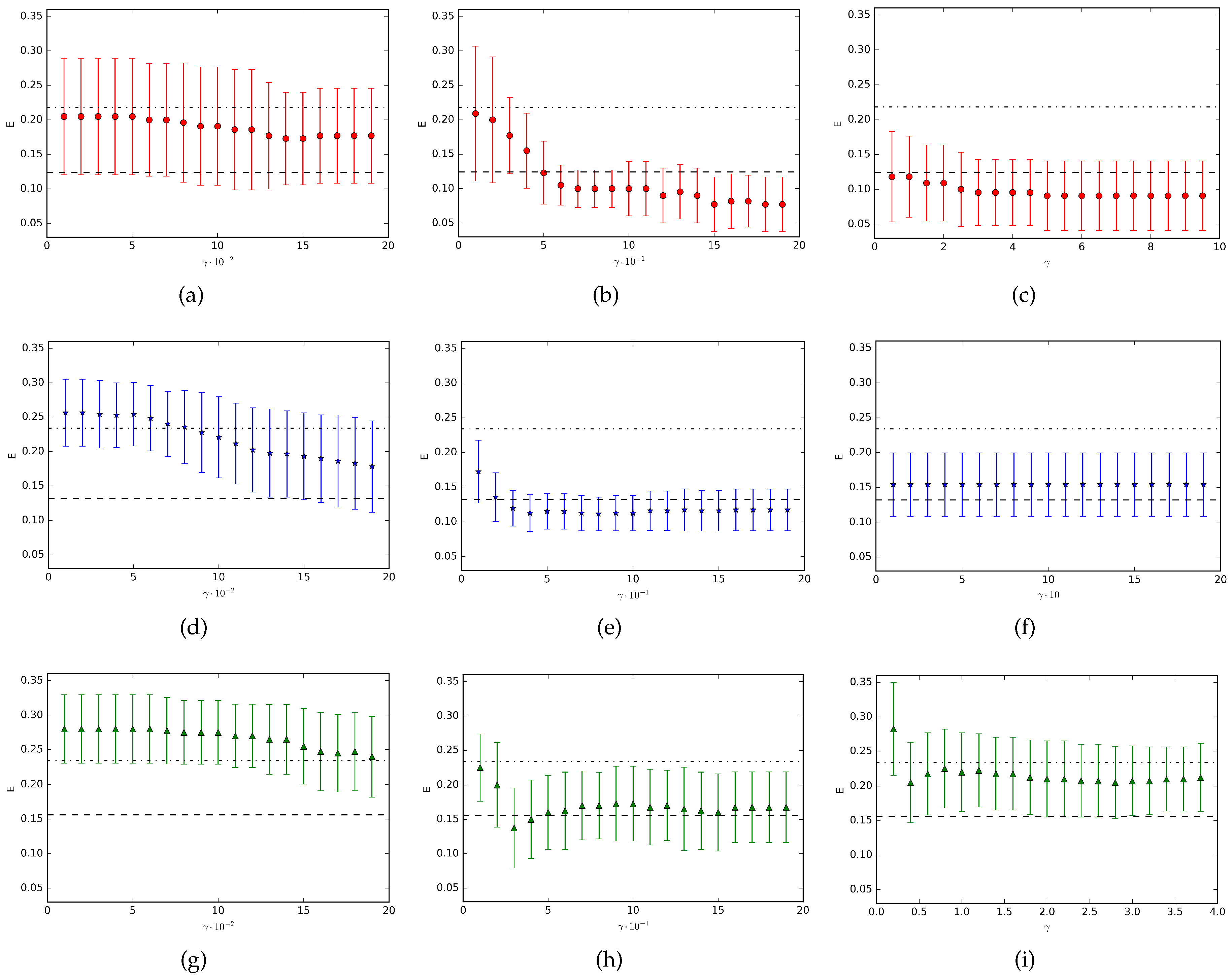
For any value of the parameter $\gamma$ it can be proved [22] that, while the NMC is invariant under rescaling, for the QNMC this invariance fails. Interestingly enough, it is possible to consider the failure of the invariance under rescaling as a resource for the classification problem. In other words, through a suitable choice of the rescaling factor is possible, in principle, to get a decreasing of the classification error. To this end, we have studied the variation of the QNMC performance (in particular of the classification error) in terms of the free parameter $\gamma$ and in Figure 1 the results for the datasets Appendicitis, Monk and Moon are shown. In the figure, each point represents the mean value (with corresponding standard deviation represented by the vertical bar) over ten runs of the experiments. Finally, we have considered, as an example, three different ranges of the rescaling parameter $\gamma$ for each dataset. We can observe that the resulting classification performance strongly depends on the $\gamma$ range. Indeed, in all the three cases we consider, we obtain completely different classification results based on different choices of the $\gamma$ values. As we can see, in some situations we observe an improvement of the QNMC performance with respect to the unrescaled problem (subfigures (b), (c), (e), (h)), in other cases we get worse classification results (subfigures (a), (d), (g), (i)) and sometimes the rescaling parameter does not offer any variation of the classification error (subfigure (f)).

In conclusion, the range of the parameter $\gamma$ for which the QNMC performance improves, is generally not unique and strongly depends on the considered dataset. As a consequence, we do not generally get an improvement in the classification process for any $\gamma$ ranges. On the contrary, there exist some intervals for the parameter $\gamma$ where the QNMC classification performance is worse than the case without rescaling. Then, each dataset has specific and unique characteristics (in complete accord to the No Free Lunch Theorem) and the incidence of the non-invariance under rescaling in the decreasing of the error, in general, should be determined by empirical evidences.

6. Conclusions and Future Developments

In this work we have introduced a quantum minimum distance classifier, named Quantum Nearest Mean Classifier, which can be seen as a quantum version of the well known Nearest Mean Classifier. In particular, it is obtained by defining a suitable encoding of real patterns, i.e., density patterns, and by recovering the trace distance between density operators.

A new encoding of real patterns into a quantum objects have been proposed, suggested by recent debates on quantum machine learning according to which, in order to avoid a loss of information caused by encoding a real vector into a quantum state, we need to consider the normalized vector keeping some information about its norm simultaneously. Secondly, we have defined the quantum centroid, i.e., the pattern chosen as the prototype of each class, which is not invariant under uniform rescaling of the original dataset (unlike the NMC) and seems to exhibit a kind of sensitivity to the data dispersion.

In the experiments, both classifiers have been compared in terms of significant statistical coefficients. In particular, we have considered 27 different datasets having different nature (real-world and artificial). Further, the non-invariance under rescaling of the QNMC has suggested to study the variation of the classification error in terms of a free parameter $\gamma$, whose variation produces a modification of the data dispersion and, consequently, of the classifier performance. In particular we have showed as, in the most of cases, the QNMC exhibits a significant decreasing of the classification error (and of the other statistical coefficients) with respect to the NMC and, for some cases, the non-invariance under rescaling can provide a positive incidence in the classification process.

Let us remark that, even if there is not an absolute superiority of QNMC with respect to the NMC, the proposed technique leads to relevant improvements in terms of pattern classification when we deal with an a priori knowledge of the data distribution.

In light of such considerations, further developments of the present work will involve the study of: (i) the optimal encoding (mapping patterns to quantum states) which ensures a better classification accuracy (at least for a finite set of data); (ii) a general method to find the suitable rescaling parameter range we can apply to a given dataset for further optimizing the classification process; and (iii) the data distribution for which our quantum classifier outperforms the NMC. Further, as discussed in Section 4, in some situations the standard NMC is not very useful as a classification model, especially when the dataset distribution is quite complex to deal with. In pattern recognition, in order to address such problems, other kinds of classification techniques are used instead of the NMC, for instance the well known Linear Discriminant Analysis (LDA) or Quadratic Discriminant Analysis (QDA) classifiers, where different distances between patterns are considered, taking the data distribution into account more precisely [24]. To this end, an interesting development of the present work could regard the comparison between the LDA or QDA models and the QNMC based on the computation of more suitable and convenient distances between density patterns [35].

References

- Aerts, D.; Sozzo, S.; Veloz, T. Quantum structure of negation and conjunction in human thought. Front. Psychol. 2015, 6, 1447. [Google Scholar] [CrossRef] [PubMed]
- Ohya, M.; Volovich, I. Mathematical Foundations of Quantum Information and Computation and Its Applications to Nano- and Bio-Systems; Springer: Dordrecht, The Netherlands, 2011; ISBN 978-94-007-0170-0. [Google Scholar]
- Stapp, H.P. Mind, Matter, and Quantum Mechanics, 3rd ed.; Springer-Verlag: Berlin, Germany, 1993. [Google Scholar]
- Wang, B.; Zhang, P.; Li, J.; Song, D.; Hou, Y.; Shang, Z. Exploration of quantum interference in document relevance judgement discrepancy. Entropy 2016, 18, 144. [Google Scholar] [CrossRef]
- Eisert, J.; Wilkens, M.; Lewenstein, M. Quantum games and quantum strategies. Phys. Rev. Lett. 1999, 83, 3077. [Google Scholar] [CrossRef]
- Haven, E.; Khrennikov, A. Quantum Social Science; Cambridge University Press: Cambridge, UK, 2013; ISBN 978-1-107-01282-0. [Google Scholar]
- Veloz, T.; Desjardins, S. Unitary Transformations in the Quantum Model for Conceptual Conjunctions and Its Application to Data Representation. Front. Psychol. 2015, 6, 1734. [Google Scholar] [CrossRef] [PubMed]
- Eldar, Y.C.; Oppenheim, A.V. Quantum signal processing. IEEE Signal Process. Mag. 2002, 19, 12–32. [Google Scholar] [CrossRef]
- Schuld, M.; Sinayskiy, I.; Petruccione, F. An introduction to quantum machine learning. Contemp. Phys. 2015, 56, 172–185. [Google Scholar] [CrossRef]
- Manju, A.; Nigam, M.J. Applications of quantum inspired computational intelligence: A survey. Artif. Intell. Rev. 2014, 42, 79–156. [Google Scholar] [CrossRef]
- Horn, D.; Gottlieb, A. Algorithm for data clustering in pattern recognition problems based on quantum mechanics. Phys. Rev. Lett. 2001, 88, 018702. [Google Scholar] [CrossRef] [PubMed]
- Liu, D.; Yang, X.; Jiang, M. A Novel Text Classifier Based on Quantum Computation. In Proceedings of the 51th Annual Meeting of the Association for Computational Linguistics, Sofia, Bulgaria, 4–9 August 2013; pp. 484–488. [Google Scholar]
- Tanaka, K.; Tsuda, K. A quantum-statistical-mechanical extension of gaussian mixture model. J. Phys. Conf. Ser. 2008, 95, 012023. [Google Scholar] [CrossRef]
- Caraiman, S.; Manta, V. Image processing using quantum computing. In Proceedings of the 16th International Conference on System Theory, Control and Computing (ICSTCC), Sinaia, Romania, 12–14 October 2012. [Google Scholar]
- Rebentrost, P.; Mohseni, M.; Lloyd, S. Quantum support vector machine for big feature and big data classification. Phys. Rev. Lett. 2014, 113. [Google Scholar] [CrossRef] [PubMed]
- Wiebe, N.; Kapoor, A.; Svore, K.M. Quantum nearest-neighbor algorithms for machine learning. Quantum Inf. Comput. 2015, 15, 0318–0358. [Google Scholar]
- Miszczak, J.A. High-level Structures for Quantum Computing. In Synthesis Lectures on Quantum Computing; Morgan & Claypool Publishers: Williston, FL, USA, 2012. [Google Scholar]
- Holik, F.; Sergioli, G.; Freytes, H.; Plastino, A. Pattern Recognition in Non-Kolmogorovian Structures. Found. Sci. 2017, 1–14. [Google Scholar] [CrossRef]
- Trugenberger, C.A. Quantum pattern recognition. Quantum Inf. Process. 2002, 1, 471–493. [Google Scholar] [CrossRef]
- Lloyd, S.; Mohseni, M.; Rebentrost, P. Quantum principal component analysis. Nat. Phys. 2014, 10, 631–633. [Google Scholar] [CrossRef]
- Sergioli, G.; Santucci, E.; Didaci, L.; Miszczak, J.A.; Giuntini, R. A quantum-inspired version of the Nearest Mean Classifier. Soft Comput. 2017, 1–15. [Google Scholar] [CrossRef]
- Sergioli, G.; Bosyk, G.M.; Santucci, E.; Giuntini, R. A quantum-inspired version of the classification problem. Int. J. Theor. Phys. 2017, 56, 3880–3888. [Google Scholar] [CrossRef]
- Santucci, E.; Sergioli, G. Classification problem in a quantum framework. In Quantum Foundations, Probability and Information, Proceedings of the Quantum and Beyond Conference, Vaxjo, Sweden, 13–16 June 2016; Khrennikov, A., Bourama, T., Eds.; Springer: Berlin, Germany, 2017; in press. [Google Scholar]
- Duda, R.O.; Hart, P.E.; Stork, D.G. Pattern Classification, 2nd ed.; Wiley: Hoboken, NJ, USA, 2000; ISBN 978-0-471-05669-0. [Google Scholar]
- Webb, A.R.; Copsey, K.D. Statistical Pattern Recognition, 3rd ed.; Wiley: Hoboken, NJ, USA, 2011; ISBN 978-0-470-68227-2. [Google Scholar]
- Johnson, R.A.; Wichern, D.W. Applied Multivariate Statistical Analysis, 6th ed.; Pearson: London, UK, 2007. [Google Scholar]
- Fawcett, T. An introduction of the ROC analysis. Pattern Recognit. Lett. 2006, 27, 861–874. [Google Scholar] [CrossRef]
- Coxeter, H.S.M. Introduction to Geometry, 2nd ed.; Wiley: Hoboken, NJ, USA, 1989. [Google Scholar]
- Kimura, G. The Bloch vector for N-level systems. Phys. Lett. A 2003, 314, 339–349. [Google Scholar] [CrossRef]
- Bertlmann, R.A.; Krammer, P. Bloch vectors for qudits. J. Phys. A Math. Theor. 2008, 41, 235303. [Google Scholar] [CrossRef]
- Karlıǧa, B. On the generalized stereographic projection. Beitr. Algebra Geom. 1996, 37, 329–336. [Google Scholar]
- Kimura, G.; Kossakowski, A. The Bloch-vector space for N-level systems: the spherical-coordinate point of view. Open Syst. Inf. Dyn. 2005, 12, 207–229. [Google Scholar] [CrossRef]
- Jakóbczyk, L.; Siennicki, M. Geometry of bloch vectors in two-qubit system. Phys. Lett. A 2001, 286, 383–390. [Google Scholar] [CrossRef]
- Nielsen, M.A.; Chuang, I.L. Quantum Computation and Quantum Information, 10th Anniversary ed.; Cambridge University Press: Cambridge, UK, 2010. [Google Scholar]
- Sommers, H.J.; Zyczkowski, K. Bures volume of the set of mixed quantum states. J. Phys. A Math. Gen. 2003, 36, 10083. [Google Scholar] [CrossRef]
- Ruskai, M.B. Beyond strong subadditivity? Improved bounds on the contraction of generalized relative entropy. Rev. Math. Phys. 1994, 6, 1147–1161. [Google Scholar] [CrossRef]
- UCL Machine Learning Repository (Center for Machine Learning and Intelligent Systems). Available online: http://archive.ics.uci.edu/ml (accessed on 30 November 2017).
- Knowledge Extraction based on Evolutionary Learning. Available online: http://sci2s.ugr.es/keel/datasets.php (accessed on 30 November 2017).
- Skurichina, M.; Duin, R.P.W. Bagging, Boosting and the Random Subspace Method for Linear Classifiers. Pattern Anal. Appl. 2002, 5, 121–135. [Google Scholar] [CrossRef]
- Wassermann, L. All of Statistic: A Concise Course in Statistical Inference; Springer: Berlin, Germany, 2004. [Google Scholar]
Figure 1.
Comparison between NMC (Nearest Mean Classifier) and QNMC (Quantum Nearest Mean Classifier) performance in terms of the classification error for the datasets (a–c) Appendicitis, (d–f) Monk, (g–i) Moon. In all the subfigures, the simple dashed line represents the QNMC classification error without rescaling, the dashed line with points represents the NMC classification error (which does not depend on the rescaling parameter), points with related error bars (red for Appendicitis, blue for Monk and green for Moon) represent the QNMC classification error for increasing values of the parameter .