Connecting Information Geometry and Geometric Mechanics

Abstract

The divergence function in information geometry, and the discrete Lagrangian in discrete geometric mechanics each induce a differential geometric structure on the product manifold $Q\times Q$. We aim to investigate the relationship between these two objects, and the fundamental role that duality, in the form of Legendre transforms, plays in both fields. By establishing an analogy between these two approaches, we will show how a fruitful cross-fertilization of techniques may arise from switching formulations based on the cotangent bundle $T^{\ast }Q$ (as in geometric mechanics) and the tangent bundle $TQ$ (as in information geometry). In particular, we establish, through variational error analysis, that the divergence function agrees with the exact discrete Lagrangian up to third order if and only if Q is a Hessian manifold.

1. Introduction

Information geometry and geometric mechanics each induce geometric structures on an arbitrary manifold Q, and we investigate the relationship between these two approaches. More specifically, we study the interaction of three objects: $TQ$, the tangent bundle on which a Lagrangian function $L(q,v)$ is defined; $T^{\ast }Q$, the cotangent bundle on which a Hamiltonian function $H(q,v)$ is defined; and $Q\times Q$, the product manifold on which the divergence function (from the information geometric perspective) or the Type I generating function (from the geometric mechanics perspective) is defined. In discrete mechanics, while the $Q\times Q⟷T^{\ast }Q$ correspondence is via a symplectomorphism given by the time-h flow map associated with the Hamiltonian $H(q,p)$, and the $Q\times Q⟷TQ$ correspondence is via the map relating the boundary-value and initial-value formulation of the Euler–Lagrange flow, it is the correspondence between $TQ⟷T^{\ast }Q$ through the fiberwise Legendre map based on L or H that actually serves to couple the Hamiltonian flow with Lagrangian flow, leading to one and the same dynamics. We propose a decoupling of the Lagrangian and Hamiltonian dynamics through the use of a divergence function $D(q,v,p)$ defined on the Pontryagin bundle $TQ\oplus T^{\ast }Q$ that measures the discrepancy (or duality gap) between $H(q,p)$ and $L(q,v)$. We also establish, through variational error analysis that the divergence function agrees with exact discrete Lagrangian up to third order if and only if Q is a Hessian manifold.

Geometric mechanics [1] investigates the equations of motion using the Lagrangian, Hamiltonian, and Hamilton–Jacobi formulations of classical Newtonian mechanics. Two apparently different principles were used in those formulations: the principle of conservation (energy, momentum, etc.) leading to Hamiltonian dynamics and the principle of variation (least action) leading to Lagrangian dynamics. The conservation properties of the Hamiltonian approach are with respect to the underlying symplectic geometry on the cotangent bundle, whereas the variational principles that result in the Euler–Lagrange equation of motions and the Hamilton–Jacobi equations reflect the geometry of the semispray on the tangent bundle. Lagrangian and Hamiltonian mechanics reflect two sides of the same coin–that they describe the identical dynamics on the configuration space (base manifold) is both remarkable and also to be expected due to their construction: because the Lagrangian and Hamiltonian are dual to each other, and related via the Legendre transform.

Information geometry [2,3] in the broadest sense of the term, provides a dualistic Riemannian geometric structure that is induced by a class of functions called divergence functions, which essentially provide a method of smoothly measuring a directed distance between any two points on the manifold, where the manifold is the space of probability densities. It arises in various branches of information science, including statistical inference, machine learning, neural computation, information theory, optimization and control, etc. Various geometric structures can be induced from divergence functions, including metric, affine connection, symplectic structure, etc., and this is reviewed in [4]. Convex duality and the Legendre transform play a key role in both constructing the divergence function and characterizing the various dualities encoded by information geometry [5,6].

Given that geometric mechanics and information geometry both prescribe dualistic geometric structures on a manifold, it is interesting to explore the extent to which these two frameworks are related. In geometric mechanics, the Legendre transform provides a link between the Hamiltonian function that is defined on the cotangent bundle $T^{\ast }Q$, with the Lagrangian function that is defined on the tangent bundle $TQ$, whereas in information geometry, it provides a link between the biorthogonal coordinates of the base manifold Q if it is dually-flat and exhibits the Hessian geometry. To understand their deep relationship, it turns out that we need to resort to the discrete formulation of geometric mechanics, and investigate the product manifold $Q\times Q$. The basic tenet of discrete geometric mechanics is to preserve the fact that Hamiltonian flow is a symplectomorphism, and construct discrete time maps that are symplectic. This results in two ways of viewing discrete-time mechanics, either as maps on $Q\times Q$ or $T^{\ast }Q$, which are related via discrete Legendre transforms. The shift in focus from $T^{\ast }Q$ to $Q\times Q$ precisely lends itself to establishing a connection to information geometry, as the divergence function is naturally defined on $Q\times Q$, and in both information geometry and discrete geometric mechanics, induces a symplectic structure on $Q\times Q$. This is the basic observation that connects geometric mechanics and information geometry, and we will explore the implications of this connection in the paper.

Our paper is organized as follows. Section 2 provides a contemporary viewpoint of geometric mechanics, with Lagrangian and Hamiltonian systems discussed in parallel with one another, in terms of geometry on $TQ$ and $T^{\ast }Q$, respectively, including a discussion of Dirac mechanics on the Pontryagin bundle $TQ\oplus T^{\ast }Q$, which provides a unified treatment of Lagrangian and Hamiltonian mechanics. Section 3 summarizes the results of the discrete formulation of geometric mechanics, which is naturally defined on the product manifold $Q\times Q$. Section 4 is a review of now-classical information geometry, including the Riemannian metric and affine connections on $TQ$, and the manner in which the divergence function naturally induces dualistic Riemannian structures. The special cases of Hessian geometry and biorthogonal coordinates are highlighted, showing how the Legendre transform is essential for characterizing dually-flat spaces. Section 5 starts with a presentation of the symplectic structure on $Q\times Q$ induced by a divergence function, which is naturally identified with the Type I generating function on it. We follow up by investigating its transformation into a Type II generating function (which plays a key role in discrete Hamiltonian mechanics). We then propose to decouple the discrete Hamiltonian and Lagrangian dynamics by using the divergence function to measure their duality gap. Finally, we perform variational error analysis to show that on a dually-flat Hessian manifold, the Bregman divergence is third-order accurate with respect to the exact discrete Lagrangian. Section 6 closes with a summary and discussion.

2. A Review of Geometric Mechanics

Consider an n-dimensional configuration manifold Q, with local coordinates $(q^1,\dots ,q^n)$. The Lagrangian formulation of mechanics is defined on the tangent bundle $TQ$, in terms of a Lagrangian $L:TQ\to \mathbb{R}$. From this, one can construct an action integral $\mathcal{S}$ which is a functional of the curve $q:[t_1,t_2]\to Q$, given by

$$\mathcal{S}\left(q\right)={\int }_{t_1}^{t_2}L(q\left(t\right),\dot{q}\left(t\right))dt.$$

Then, Hamilton’s variational principle states that,

$$\delta \mathcal{S}\left(q\right)=0,$$

(1)

where the variation $\delta \mathcal{S}$ is induced by an infinitesimal variation $\delta q$ of the trajectory q, subject to the condition that the variations vanish at the endpoints, i.e., $\delta q\left(t_1\right)=\delta q\left(t_2\right)=0$. Applying standard results from the calculus of variations, we obtain the following Euler–Lagrange equations of motion,

$$\frac{d}{dt}\frac{\partial L}{\partial {\dot{q}}^i}-\frac{\partial L}{\partial q^i}=0.$$

(2)

The Hamiltonian formulation of mechanics is defined on the cotangent bundle $T^{\ast }Q$, and the fiberwise Legendre transform, $\mathbb{F}L:TQ\to T^{\ast }Q$, relates the tangent bundle and the cotangent bundle as follows,

$$(q^i,{\dot{q}}^i)\mapsto (q^i,p_i)=\left(q^i,\frac{\partial L}{\partial {\dot{q}}^i}\right),$$

where $p_i$ is the conjugate momentum to $q^i$:

$$p=\frac{\partial L}{\partial \dot{q}}.$$

(3)

The term fiberwise is used to emphasize the fact that $\mathbb{F}L$ establishes a pointwise correspondence between $T_{q}Q$ and $T_q^{\ast }Q$ for any point q on Q. The cotangent bundle forms the phase space, on which one can define a Hamiltonian $H:T^{\ast }Q\to \mathbb{R}$,

$$H(q,p)=⟨p,\dot{q}(q,p)⟩-L(q,\dot{q}(q,p)),$$

where $\dot{q}$ is viewed as a function of $(q,p)$ by inverting the Legendre transform (3), and

$${⟨p,v⟩}_q=\sum _i{p}_i{v}^i$$

denotes the duality or natural pairing between a vector v and covector p at the point $q\in Q$. A straightforward calculation shows that

$$\frac{\partial H}{\partial p_i}={\dot{q}}^i,$$

(4)

and

$$\frac{\partial H}{\partial q^i}=-\frac{\partial L}{\partial q^i}.$$

From these, we transform the Euler–Lagrange equations into Hamilton’s equations,

$$\frac{d{q}^i}{dt}=\frac{\partial H}{\partial p_i},\frac{d{p}_i}{dt}=-\frac{\partial H}{\partial q^i}.$$

(5)

The canonical symplectic form ${\omega }_{can}$ on $T^{\ast }M$ can be identified with a quadratic form induced by the skew-symmetric matrix J, i.e., ${\omega }_{can}(v,w)=v^{T}Jw$. With that identification, Hamilton’s equations can be expressed as,

$$\left[\begin{array}{c}\dot{q}\\ \dot{p}\end{array}\right]=\left[\begin{array}{cc}0& \mathrm{I}\\ -\mathrm{I}& 0\end{array}\right]\left[\begin{array}{c}\frac{\partial H}{\partial q}\\ \frac{\partial H}{\partial p}\end{array}\right]=J\left[\begin{array}{c}\frac{\partial H}{\partial q}\\ \frac{\partial H}{\partial p}\end{array}\right].$$

Alternatively, Hamilton’s equations (5) can be derived using Hamilton’s phase space variational principle, which states that,

$$\delta {\int }_{t_1}^{t_2}\left[⟨p,\dot{q}⟩-H(q,p)\right]dt=0,$$

for infinitesimal variations $\delta q$ that vanish at the endpoints. The infinitesimal variation of the integral is computed by differentiating under the integral, integrating by parts, and using the fact that the infinitesimal variations $\delta q$ vanish at the endpoints, which yields:

$${\int }_{t_1}^{t_2}\left(⟨\delta p,\dot{q}⟩+⟨p,\delta \dot{q}⟩-\frac{\partial H}{\partial q}\delta q-\frac{\partial H}{\partial p}\delta p\right)dt={\int }_{t_1}^{t_2}\left[\left(-\dot{p}-\frac{\partial H}{\partial q}\right)\delta q+\left(\dot{q}-\frac{\partial H}{\partial p}\right)\delta p\right]dt,$$

and by the fundamental theorem of the calculus of variations, which states that the integral is stationary only when the terms in the parentheses multiplying into the independent variations $\delta q$ and $\delta p$ vanish, we recover Hamilton’s equations (5).

Lagrangian and Hamiltonian mechanics are typically viewed as different representations of the same dynamical system, with the Legendre transform relating the two formulations. Here, the Legendre transform $\mathbb{F}L$ (with $\mathbb{F}H$ as its inverse) refers to both the map relating two sets of variables, $(q,\dot{q})$ with $(q,p)$, as well as the relationship between two functions, the Lagrangian $L(q,\dot{q})$ and the Hamiltonian $H(q,p)$. The Legendre transform links pairs of convex conjugate functions; in classical mechanics, the Lagrangian L and Hamiltonian H are always related in this sense of forming a convex pair. The requirement that $L(q,\dot{q})$ be strictly convex in the variable $\dot{q}$ is referred to as hyperregularity. When the Lagrangian is positive homogeneous (or singular), the Legendre transform yields a Hamiltonian function that is identically zero, which means that in such cases, the Hamiltonian analogue of the Lagrangian system does not exist, which is problematic in the context of analytic mechanics. In order to address such degeneracy, it is necessary to consider Dirac mechanics on Dirac manifolds, which is a simultaneous generalization of Lagrangian and Hamiltonian mechanics.

In geometric mechanics, including the contemporaneous Dirac formulation, the Lagrangian L and Hamiltonian H are always coupled via the fiberwise Legendre transform $\mathbb{F}L$. In information geometry, it is a well-known fact that one can construct the divergence function (to be defined later), which captures the departure from such perfect coupling. In other words, we can view Lagrangian and Hamiltonian systems as two separate systems, which are endowed with their own dynamics and are in some sense dual to each other, and we then use the divergence function to measure their duality gap. For this reason, we will review the Lagrangian and Hamiltonian formulation of mechanics in terms of $L(q,\dot{q})$ and $H(q,p)$, respectively, without necessarily assuming that the Lagrangian and Hamiltonian are related by the Legendre transform.

2.1. Lagrangian Mechanics as an Extremization System on $TQ$

As noted previously, the Euler–Lagrange equations (2) arise from the stationarity conditions that describe the extremal curves of the action integral, over the class of varied curves that fix the endpoints. Carrying out the differentiation in (2) explicitly yields,

$$\sum _j\frac{{\partial }^{2}L}{\partial v^i\partial v^j}\frac{d{v}^j}{dt}+\sum _j{v}^j\frac{{\partial }^{2}L}{\partial q^j\partial v^i}-\frac{\partial L}{\partial q^i}=0.$$

(6)

The fundamental tensor $g_{ij}$ associated with the Lagrangian $L(q,v)$ is given by,

$$g_{ij}(q,v)=\frac{{\partial }^{2}L(q,v)}{\partial v^i\partial v^j},$$

which is assumed to be positive-definite, i.e., the Lagrangian L is hyperregular. Let $g^{il}$ denote the matrix inverse of $g_{ij}$, then (6) can be written as

$$\frac{d^2{q}^i}{d{t}^2}+2G^i\left(q,\frac{dq}{dt}\right)=0,$$

(7)

where

$$G^i(q,v)=\sum _l\frac{g^{il}}{2}\left(\sum _k\frac{{\partial }^{2}L}{\partial q^k\partial v^l}{v}^k-\frac{\partial L}{\partial q^l}\right).$$

So, Equation (7) with the above $G^i$ are Euler–Lagrange equations in disguise, and its solution is an extremal curve of the action integral.

Recall that a smooth curve on Q can be lifted to a curve on $TQ$ in a natural way: a curve $t\mapsto q\left(t\right)\in Q$ becomes $t\mapsto (q\left(t\right),\dot{q}\left(t\right))\in TQ$. Given an arbitrary $G^i(q,v)$, the system of equations (7) specify a family of curves, called a semispray. As seen above, semisprays arise naturally in variational calculus as extremal curves of the action integral associated with a Lagrangian.

Semisprays can be more generally described by a vector field. Recall that a vector field on Q is a section of $TQ$. Now, consider a vector field on the tangent bundle $TQ$; it is a section of the double tangent bundle $T\left(TQ\right)$. The integral surfaces of the semispray induces a decomposition of the total space $T\left(TQ\right)$ into the horizontal subspace $\mathcal{H}\left(TQ\right)$ and the vertical subspace $\mathcal{V}\left(TQ\right)$, which defines an Ehresmann connection. A vector on $TQ$ encodes the second-order derivative of curves on Q, and a semispray defines the following vector field V on $TQ$:

$$V(q,v)=\sum _i\left(v^i{\left.\frac{\partial }{\partial q^i}\right|}_{(q,v)}-2G^i(q,v){\left.\frac{\partial }{\partial v^i}\right|}_{(q,v)}\right),$$

where the factor $-2$ is there by convention. The integral curve of the semispray satisfies the second-order ordinary differential equation (7), and we say that a semispray is a vector field on the tangent bundle $TQ$ which encodes a second-order system of differential equations on the base manifold Q.

A semispray is called a full spray if the spray coefficients $G^i$ satisfy

$$G^i(q,\lambda v)={\lambda }^2{G}^i(q,v),$$

for $\lambda >0$. In this case, the integral curve remains invariant under reparameterization by a positive number, i.e., it satisfies homogeneity. When the semispray becomes a (full) spray, the Lagrange geometry becomes Finsler geometry, and the fundamental tensor $g_{ij}(q,v)$ becomes the Finsler–Riemann metric tensor (which includes the Riemann metric as a special case).

As noted above, a semispray induces an Ehresmann connection on Q and this connection is torsion-free and typically nonlinear. Conversely, given a torsion-free connection, one can construct a semispray. The connection is homogenous if and only if the semispray is a full spray. Moreover, if the spray is affine, then the connection is affine as well—an affine spray $G^i$ takes the form

$$G^i=\frac{1}{2}\sum _{jk}{\Gamma }_{jk}^i\left(q\right)v^j{v}^k,$$

where ${\Gamma }_{jk}^i$ is referred to as the affine connection.

To summarize, Lagrangian dynamics is related to action minimization by the Euler operator, and leads to a semispray on the configuration manifold Q. Under suitable conditions, the Lagrangian function $L(q,v)$ defined on $TQ$ will lead to a torsion-free but generally nonlinear connection, and an affine connection only for a very special form of Lagrangian.

2.2. Hamiltonian Mechanics as a Conservative System on $T^{\ast }Q$

Given a Hamiltonian $H:T^{\ast }Q\to \mathbb{R}$, we consider the Hamiltonian vector field $X_H\in \mathfrak{X}\left(T^{\ast }Q\right)$ (where $\mathfrak{X}$ denotes a section) defined by

$$X_H=\left(\frac{\partial H}{\partial p_i},-\frac{\partial H}{\partial q^i}\right).$$

(8)

It is straightforward to verify that $H=const$ along the dynamical flow of $X_H$:

$$\frac{dH}{dt}=\sum _i\left(\frac{\partial H}{\partial q^i}\frac{d{q}^i}{dt}+\frac{\partial H}{\partial p_i}\frac{d{p}_i}{dt}\right)=0.$$

So, a Hamiltonian vector field $X_H$ advects the Hamiltonian H along its flow, so that H is constant along solution curves, which implies that the Lie derivative $\mathcal{L}$ of H along the flow of $X_H$ vanishes,

$${\mathcal{L}}_{X_H}H=0.$$

Formally, starting from the tautological 1-form $\theta ={\sum }_i{p}_{i}d{q}^i$ on Q, one obtains a 2-form $\omega$, called the Poincaré 2-form,

$$\omega =-d\theta =\sum _{i}d{q}^i\wedge d{p}_i,$$

which is the canonical symplectic form on $T^{\ast }Q$:

$$\omega (X,Y)=\sum _i(d{q}^i\wedge d{p}_i)(X,Y)=\sum _i\left(\frac{\partial X}{\partial q^i}\frac{\partial Y}{\partial p_i}-\frac{\partial X}{\partial p_i}\frac{\partial Y}{\partial q^i}\right),$$

where $X,Y$ are vector fields on $T^{\ast }Q$.

More generally, given a Hamiltonian H along with a symplectic form $\omega$, which is, by definition, a closed, nondegenerate 2-form, one obtains the Hamiltonian vector field $X_H$ on $T^{\ast }Q$, defined in abstract notation by

$${\iota }_{X_H}\omega =dH,$$

(9)

or equivalently in a more familiar notation,

$$\omega (X_H,·)=dH(·).$$

One can define the Poisson bracket $\{·,·\}$ of two functions F and G by using their respective Hamiltonian vector fields and the symplectic form,

$$\{F,G\}\equiv \omega (X_F,X_G).$$

For the canonical symplectic form, it has the following coordinate expression,

$$\{F,G\}=\sum _i\left(\frac{\partial F}{\partial q^i}\frac{\partial G}{\partial p_i}-\frac{\partial F}{\partial p_i}\frac{\partial G}{\partial q^i}\right).$$

In this way, Hamilton’s equations can be expressed in terms of the Poisson bracket as follows,

$$\frac{d{q}^i}{dt}=\{q^i,H\},\frac{d{p}^i}{dt}=\{p^i,H\}.$$

(10)

By Darboux’s theorem, it is always possible to choose local coordinates $(q,p)$ on $T^{\ast }Q$, referred to as canonical coordinates, such that the symplectic form has the expression $\omega ={\sum }_{i}d{q}^i\wedge d{p}_i$. In these coordinates, Hamilton’s equations defined in terms of the symplectic structure (9) and Poisson structure (10) recover the canonical Hamiltonian vector field (8).

Note that any smooth function H on $T^{\ast }Q$ induces a Hamiltonian vector field. An arbitrary vector field X on $T^{\ast }Q$ is locally Hamiltonian, i.e., induced by a smooth function H, if ${\iota }_X\omega$ is closed, i.e., ${\mathcal{L}}_X\omega =0$. In addition, a Hamiltonian vector field preserves the volume form $\mathsf{\Omega }$, i.e.,

$${\mathcal{L}}_X\left(\mathsf{\Omega }\right)=0,$$

where $\mathsf{\Omega }$ is the n-fold exterior product of $\omega$,

$$\mathsf{\Omega }=\frac{{(-1)}^{\frac{n(n-1)}{2}}}{n!}\omega \wedge \omega \cdots \wedge \omega .$$

2.3. Symplectic Maps and Symplectic Flows

A symplectic map is a diffeomorphism of $T^{\ast }Q$ that preserves its symplectic structure $\omega$. We first consider a one-parameter family of symplectic maps generated by the flow map $F_X:T^{\ast }Q\to T^{\ast }Q$ of a vector field $X\in \mathfrak{X}\left(T^{\ast }Q\right)$. Since the entire family of symplectic maps leave $\omega$ invariant, it follows that ${\pounds }_X\omega =0$. It can be shown (using Cartan’s magic formula, and the fact that $\omega$ is closed) that a vector field $X\in \mathfrak{X}\left(T^{\ast }Q\right)$ is symplectic if $i_X\omega$ is closed, i.e., $d\left(i_X\omega \right)=0$. By the Poincaré lemma, this implies that $i_X\omega$ is locally exact, that is, in the neighborhood of any point, there exists some function $H:T^{\ast }Q\to \mathbb{R}$ such that $i_X\omega =dH$. So there is always locally exists a Hamiltonian $H:T^{\ast }Q\to \mathbb{R}$ that generates a vector field X whose flow is symplectic with respect to $\omega$.

More generally, a diffeomorphism $\varphi :M_1\to M_2$ is a symplectic map from a symplectic space $(M_1,{\omega }_1)$ to another space $(M_2,{\omega }_2)$ if:

$${\varphi }^{\ast }{\omega }_2={\omega }_1,$$

(11)

where ${\omega }_1,{\omega }_2$ are the symplectic forms on $M_1,M_2$, respectively. The above condition (11) holds if and only if for any functions f, g:

(i)

$\{f,g\}\circ \varphi =\{f\circ \varphi ,g\circ \varphi \}$,

(ii)

${\varphi }^{\ast }{X}_H=X_{H\circ \varphi }$.

With respect to Darboux coordinates about a point $z=(q,p)\in M_1$, the condition (11) that a map $\varphi :M_1\to M_2$ is symplectic can be expressed locally by ${\left(D_z\varphi \right)}^{T}J\left(D_z\varphi \right)=J$, where $D_{z}F$ denotes the Jacobian of $\varphi$ at z.

A canonical transformation of $T^{\ast }M$ is an automorphism $\varphi :T^{\ast }Q\to T^{\ast }Q$,

$$\varphi :\left\{\begin{array}{c}(q,p)\to {\left(q^{\prime }\right)}^i(q^1,\cdots ,q^n,p_1,\cdots ,p_n),\hfill \\ (q,p)\to {\left(p^{\prime }\right)}^i(q^1,\cdots ,q^n,p_1,\cdots ,p_n),\hfill \end{array}\right.$$

such that

$$\omega =\sum _{i}d{q}^i\wedge d{p}_i=\sum _{i}d{q}^{\prime i}\wedge d{p}_i^{\prime }.$$

The significance of canonical transformations is that they preserve the form of Hamilton’s equations, and one can check that an automorphism $\varphi$ is canonical by verifying that ${\left(D_z\varphi \right)}^{T}J\left(D_z\varphi \right)=J$ in a Darboux coordinate chart.

2.4. Symplectic Structure on $TQ$ Pulled Back from $T^{\ast }Q$

If we endow $T^{\ast }Q$ with the canonical symplectic form, we can construct a symplectic form on $TQ$ in such a way that these two spaces are symplectomorphic.

The mapping between $TQ$ and $T^{\ast }Q$ can be constructed in two different ways, Case I involves the Legendre transform:

$$\begin{array}{ccc}TQ& ⟷& T^{\ast }Q\\ (q,v)& \mapsto & \left(q,\frac{\partial L(q,v)}{\partial v}\right)\\ \left(q,\frac{\partial H(q,p)}{\partial p}\right)& ↤& (q,p)\end{array}$$

(12)

and Case II involves the Riemannian metric tensor g (on Q):

$$\begin{array}{ccc}TQ& ⟷& T^{\ast }Q\\ (q,v)& \mapsto & \left(q,\sum _j{g}_{ij}{v}^j\right)\\ \left(q,\sum _j{g}^{ij}{p}_j\right)& ↤& (q,p)\end{array}$$

(13)

Note that we say that g is a pseudo-Riemannian metric on Q when g acts on a pair of tangent vectors at the tangent space $T_{q}Q$ at a point q of Q; it can be viewed as a symmetric $(0,2)$-tensor that maps $TQ\times TQ\to \mathbb{R}$. On the other hand, the symplectic form $\omega$ is a skew-symmetric $(0,2)$-tensor that acts on a pair of tangent vectors on $T^{\ast }Q$, so it maps $T\left(T^{\ast }Q\right)\times T\left(T^{\ast }Q\right)\to \mathbb{R}$.

Case I. Given the Lagrangian $L:TQ\to \mathbb{R}$, this induces the fiberwise Legendre transform $\mathbb{F}L:TQ\to T^{\ast }Q$, which is given by $(q,v)\mapsto (q,p)=\left(q,\frac{\partial L}{\partial v}\right)$. If L is hyperregular, then this map is a diffeomorphism. If we endow $TQ$ with the pullback symplectic form ${\left(\mathbb{F}L\right)}^{\ast }\omega$, which is given by

$$\sum _{ij}\frac{{\partial }^{2}L}{\partial v^j\partial v^i}d{q}^i\wedge d{v}^j+\sum _{ij}\frac{{\partial }^{2}L}{\partial q^i\partial v^j}d{q}^i\wedge d{q}^j,$$

then the Legendre transform is a symplectomorphism (by construction).

Case II. The Riemannian metric g induces the musical isomorphisms $♭:TQ\to T^{\ast }Q$ and $♯:T^{\ast }Q\to TQ$ between $TQ$ and $T^{\ast }Q$, which are the operations that lower and raise the index, respectively. If we endow $TQ$ with the pullback symplectic form ${♭}^{\ast }\omega$, which is given by

$$\omega =dq\wedge dp(q,v)=\sum _{i,j}{g}_{ij}d{q}^i\wedge d{v}^j+\sum _{ijk}\frac{\partial g_{ij}}{\partial q^k}{v}^{i}d{q}^j\wedge d{q}^k,$$

then the musical isomorphism is a symplectomorphism (by construction).

Link between Case I and Case II. It is possible that the two ways of identifying $TQ\leftrightarrow T^{\ast }Q$ may be the same; this happens when g on $TQ$ coincides with the second derivatives of $L(q,v)$ with respect to the v-variable:

$$g_{ij}(q,v)=\frac{{\partial }^{2}L(q,v)}{\partial v_i\partial v_j},$$

assuming L is hyperregular. The inverse of g, denoted $\tilde{g}$, can be obtained from

$${\tilde{g}}^{ij}(q,p)=\frac{{\partial }^{2}H(q,p)}{\partial p_i\partial p_j},$$

using the Hamiltonian $H(q,p)$ defined on $T^{\ast }Q$. Note that when the Lagrangian has the form $L(q,v)=\frac{1}{2}{v}^{T}M\left(q\right)v-V\left(q\right)$, this corresponds to the Riemannian metric g being given by the kinetic energy metric $M\left(q\right)$.

2.5. Hamilton-Jacobi Theory and Dirichlet-to-Neumann Map

In classical mechanics, the Hamilton–Jacobi equation is first introduced as a partial differential equation that the action integral satisfies. Recall that the action integral S along the solution of the Euler–Lagrange equation (2) over the time interval $[t_0,t]$ is

$$S_{q_0}\left(q\left(t\right)\right):={\int }_{t_0}^{t}L(q\left(s\right),\dot{q}\left(s\right))ds, \mathrm{where}q(·)\text{is the solution of the Euler–Lagrange equation}.$$

(14)

This is referred to as Jacobi’s solution of the Hamilton–Jacobi equation. Here, we assume that the initial position $q\left(0\right)$ is fixed and the final position $q\left(t\right)$ depends on the initial velocity $v_0=\dot{q}\left(0\right)$. By taking a variation $\delta q\left(t\right)$ of the endpoint $q\left(t\right)$, one obtains a partial differential equation satisfied by $S(q,t)$:

$$H\left(q,\frac{\partial S}{\partial q}\right)=0.$$

(15)

This is the Hamilton–Jacobi equation, when H does not explicit depend on t.

Conversely, it is shown that if $S_{q_0}\left(q\right)$ is a solution of the Hamilton–Jacobi equation then $S_{q_0}\left(q\right)$ is a generating function for the family of canonical transformations (or symplectic flows) that describe the dynamics defined by Hamilton’s equations. This result is the theoretical basis for the powerful technique of exact integration called separation of variables.

There are two uses of $S_{q_0}\left(q\right)$. First, it serves to characterize the Dirichlet-to-Neumann map, which refers to the correspondence between the boundary data $(q_0,q)\in Q\times Q$ with the initial data $(q_0,v_0)\in TQ$ of a dynamical system. Second, it provides a foliation of the configuration space Q, around the point $q_0$ and parameterized by t, that is defined by the condition $S_{q_0}\left(q\left(t\right)\right)=const$.

In the rest of the paper, we will view $S_{q_0}\left(q\right)$ as a scalar-valued function of $(q_0,q\left(t\right))$, which we refer to as the exact discrete Lagrangian $L_d^E:Q\times Q\to \mathbb{R}$,

$$L_d^E(q_0,q_1;h)=\underset{\begin{array}{c}q\in C^2([0,h],Q)\\ q\left(0\right)=q_0,q\left(h\right)=q_1\end{array}}{ext}{\int }_0^{h}L(q\left(t\right),\dot{q}\left(t\right))dt.$$

(16)

this is equivalent to the expression for Jacobi’s solution, as the stationarity conditions of this variational characterization are simply the Euler–Lagrange equations. Furthermore, this characterization has the added benefit that it is well-defined even if the Lagrangian is degenerate. The exact discrete Lagrangian provides us with the time-h flow map for the Euler–Lagrange equation. Given a fixed initial point $q_0$, this defines a map which takes $q\in Q$ to an initial velocity $v_0$, such that the Euler–Lagrange trajectory $q\left(t\right)$ with initial condition $(q\left(0\right),\dot{q}\left(0\right))=(q_0,v_0)$ has boundary values $(q\left(0\right),q\left(h\right))=(q_0,q)$. This is the Dirichlet-to-Neumann map $Q\times Q\mapsto TQ$, $(q_0,q)\mapsto (q_0,v_0)$.

To address the Dirichlet-to-Neumann map more generally, let us first recall the definition of a retraction:

Definition 1

([7], Definition 4.1.1 on p. 55). A retraction on a manifold Q is a smooth mapping $\mathcal{R}$: $TQ\to Q$ with the following properties: Let ${\mathcal{R}}_q:T_{q}Q\to Q$ be the restriction of $\mathcal{R}$ to $T_{q}Q$ for an arbitrary $q\in Q$; then,

(i) 

${\mathcal{R}}_q\left(0_q\right)=q$, where $0_q$ denotes the zero element of $T_{q}Q$;

(ii) 

with the identification $T_{0_q}\left(T_{q}Q\right)\simeq T_{q}Q$, ${\mathcal{R}}_q$ satisfies

$$T_{0_q}{\mathcal{R}}_q={id}_{T_{q}Q},$$

(17)

where $T_{0_q}{\mathcal{R}}_q$ is the tangent map of ${\mathcal{R}}_q$ at $0_q\in T_{q}Q$.

Equation (17) implies that the map ${\mathcal{R}}_q:T_{q}Q\to Q$ is invertible in some neighborhood of $0_q$ in $T_{q}Q$. Its inverse is conveniently denoted as $\tilde{\mathcal{R}}:TQ\to Q\times Q$, which is defined by

$$\tilde{\mathcal{R}}\left(v_q\right):=(q,{\mathcal{R}}_q\left(v_q\right)).$$

(18)

it is easy to see that $\tilde{\mathcal{R}}:TQ\to Q\times Q$ is also invertible in some neighborhood of $0_q\in TQ$ for any $q\in Q$.

Let us introduce a special class of coordinate charts that are compatible with a given retraction map $\mathcal{R}:TQ\to Q$. A coordinate chart $(U,\phi )$ with U an open subset in Q and $\phi :U\to {\mathbb{R}}^n$ is said to be retraction compatible at $q\in U$ if

(i)

$\phi$ is centered at q, i.e., $\phi \left(q\right)=0$;

(ii)

the compatibility condition

$$\mathcal{R}\left(v_q\right)={\phi }^{-1}\circ T_q\phi \left(v_q\right)$$

(19)

holds, where we identify $T_0{\mathbb{R}}^n$ with ${\mathbb{R}}^n$ as follows: Let $\phi =(q^1,\cdots ,q^n)$ with $q^i:U\to \mathbb{R}$ for $i=1,\cdots ,n$. Then

$$v^i{\displaystyle \frac{\partial }{\partial q^i}}\mapsto (v^1,\cdots ,v^n),$$

(20)

where $\partial /\partial q^i$ is the unit vector in the $q^i$-direction in $T_0{\mathbb{R}}^n$.

An atlas for the manifold Q is retraction compatible if it consists of retraction compatible coordinate charts.

In Equation (19), we assumed that $T_q\phi \left(v_q\right)\in \phi \left(U\right)\subset {\mathbb{R}}^n$ and so strictly speaking ${\mathcal{R}}_q$ is defined on ${\left(T_q\phi \right)}^{-1}\left(\phi \left(U\right)\right)\subset T_{q}Q$. However, it is always possible to define a coordinate chart such that $\phi \left(U\right)={\mathbb{R}}^n$ by stretching out the open set $\phi \left(U\right)$ to ${\mathbb{R}}^n$ so that (19) is defined for any $v_q\in T_{q}Q$.

Retraction maps provide general means to relate $Q\times Q$ to $TQ$: in essence it provides a correspondence between $\left\{q\right\}\times Q$ and $T_{q}Q$ for all $q\in Q$ (we may take $q\in Q$ to mean the projection of $Q\times Q$ onto either the first or the second slot).

2.6. Variational Mechanics and the Pontryagin Bundle

Lagrangian and Hamiltonian mechanics can be combined into Dirac mechanics [8,9], which is described on the Pontryagin bundle $TQ\oplus T^{\ast }Q$, which has position, velocity, and momentum as local coordinates.

Just as the Euler–Lagrange equations of motion arises out of Hamilton’s principle, Hamilton’s equations can also arise from Hamilton’s phase space principle:

$$\delta {\int }_{t_1}^{t_2}\left[⟨p,\dot{q}⟩-H(q,p)\right]dt=0.$$

On the Pontryagin bundle $TQ\oplus T^{\ast }Q$, which has local coordinates $(q,v,p)$, a relaxation of Hamilton’s principle (1) is the Hamilton–Pontryagin variational principle, which uses a Lagrange multiplier p to impose the second-order condition $v=\dot{q}$,

$$\delta {\int }_{t_1}^{t_2}\left(L(q,v)-{⟨p,\dot{q}-v⟩}_q\right)dt=0.$$

(21)

This encapsulates both Hamilton’s and Hamilton’s phase space variational principles, as well as the Legendre transform, and gives the implicit Euler–Lagrange equations,

$$\dot{q}=v,\dot{p}=\frac{\partial L}{\partial q},p=\frac{\partial L}{\partial v}.$$

The last equation explicitly imposes the primary constraint condition, which is important when describing degenerate Lagrangian systems, such as electrical circuits. Note that the p are interpreted as Lagrange multipliers [10] in addition to its usual interpretation as conjugate momenta. The three equations can be combined by eliminating v and p to recover the Euler–Lagrange equations.

An important application of Hamilton–Jacobi theory is in optimal control theory. Consider a typical optimal control problem,

$$\underset{u(·)}{min}{\int }_0^{T}L(q,u)dt,$$

subject to the constraints,

$$\dot{q}=f(q,u),$$

and the boundary conditions $q\left(0\right)=q_0$ and $q\left(T\right)=q_T$. We convert constrained optimization to unconstrained optimization by using Lagrange multipliers p (sometimes called the costate or auxiliary variables), and we can define the augmented cost functional:

$$\widehat{S}\left[u\right]:={\int }_0^T\left\{L(q,u)+⟨p,\dot{q}-f(q,u)⟩\right\}dt={\int }_0^T\left\{⟨p,\dot{q}⟩-\widehat{H}(q,p,u)\right\}dt,$$

where we introduced the costate variables p, and also defined the control Hamiltonian,

$$\widehat{H}(q,p,u):=⟨p,f(q,u)⟩-L(q,u).$$

The variables $(q,p)$ forms a Hamiltonian system, so we impose the optimality condition,

$${\displaystyle \frac{\partial \widehat{H}}{\partial u}}(q,p,u)=0,$$

to obtain the equation for the optimal control $u=u^{\ast }(q,p)$, and we obtain the Hamiltonian,

$$H(q,p):=\underset{u}{max}\widehat{H}(q,p,u)=\widehat{H}(q,p,u^{\ast }(q,p)).$$

We also define the optimal cost-to-go function,

$$\begin{array}{cc}\hfill C(q,t)& :={\int }_t^T\left\{L(\widehat{q},u^{\ast })+⟨p,\dot{\widehat{q}}-f(\widehat{q},u^{\ast })⟩\right\}ds\hfill \\ & ={\int }_t^T\left\{⟨\widehat{p},\dot{\widehat{q}}⟩-H(\widehat{q},\widehat{p})\right\}ds=S^{\ast }-S(q,t),\hfill \end{array}$$

where $(\widehat{q}\left(s\right),\widehat{p}\left(s\right))$ for $s\in [0,T]$ is the solution of Hamilton’s equations with the above H such that $\widehat{q}\left(t\right)=q$; and $S^{\ast }$ is the optimal cost

$$S^{\ast }:={\int }_0^T\left\{⟨\widehat{p},\dot{\widehat{q}}⟩-H(\widehat{q},\widehat{p})\right\}ds={\int }_0^T\left\{⟨\widehat{p},\dot{\widehat{q}}⟩-\widehat{H}(\widehat{q},\widehat{p},u^{\ast }(\widehat{q},\widehat{p}))\right\}ds=\widehat{S}\left[u^{\ast }\right],$$

and the function $S(q,t)$ is defined by

$$S(q,t):={\int }_0^t\left\{⟨\widehat{p},\dot{\widehat{q}}⟩-H(\widehat{q},\widehat{p})\right\}ds.$$

Since this definition coincides with (14), the function $S(q,t)=S^{\ast }-C(q,t)$ satisfies the Hamilton–Jacobi equation (15); this reduces to the Hamilton–Jacobi–Bellman (HJB) equation for the optimal cost-to-go function $C(q,t)$:

$${\displaystyle \frac{\partial C}{\partial t}}+\underset{u}{min}\left\{⟨{\displaystyle \frac{\partial C}{\partial q}},f(q,u)⟩+L(q,u)\right\}=0.$$

(22)

It can also be shown that the costate p of the optimal solution is related to the solution of the Hamilton–Jacobi–Bellman equation.

3. Discrete Formulation of Geometric Mechanics

In this section, we review various schemes for discretizing mechanics (see, e.g., [11]). Geometric mechanics focuses on the differential geometric structure of the configuration manifolds, the associated symplectic and Poisson structures on the phase space, and the conservation laws generated by symmetries, and geometric structure-preserving numerical integration aims to preserve as many of these geometric properties as possible under discretization. The main idea is to start from the canonical symplectic form $\omega$ on $T^{\ast }Q$, and look at the symplectomorphisms that preserve $\omega$ or its pullback via the Legendre transforms to $Q\times Q$ or $TQ$.

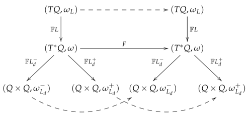
3.1. Symplectomorphisms from $T^{\ast }Q$ to $TQ$ and to $Q\times Q$

Given a cotangent bundle $T^{\ast }Q$ with a symplectic form $\omega$, we wish to endow the bundles $TQ$ and $Q\times Q$ with a symplectic structure. Given a function $L:TQ\to \mathbb{R}$, the Legendre transform is viewed as the fiber derivative $\mathbb{F}L:TQ\to T^{\ast }Q$, $(q,\dot{q})\mapsto (q,\partial L/\partial \dot{q})$. The pullback of $\omega$ with respect to $\mathbb{F}L$ yields a symplectic structure ${\omega }_L=\mathbb{F}{L}^{\ast }\omega$ on $TQ$.

Similarly, given a function $L_d:Q\times Q\to \mathbb{R}$, we define two discrete fiber derivatives, $\mathbb{F}{L}_d^{\pm }$: $Q\times Q\to T^{\ast }Q$, which serve as discrete Legendre transforms:

$$\begin{array}{cc}\hfill \mathbb{F}{L}_d^{+}(q_k,q_{k+1})& =(q_{k+1},D_2{L}_d(q_k,q_{k+1})),\hfill \end{array}$$

(23)

$$\begin{array}{cc}\hfill \mathbb{F}{L}_d^{-}(q_k,q_{k+1})& =(q_k,-D_1{L}_d(q_k,q_{k+1})).\hfill \end{array}$$

(24)

Here $D_1,D_2$ refers to taking a derivative with respect to the first or second slot, respectively:

$$D_1{L}_d(q_k,q_{k+1})=\frac{\partial L_d(q_k,q_{k+1})}{\partial q_k},D_2{L}_d(q_k,q_{k+1})=\frac{\partial L_d(q_k,q_{k+1})}{\partial q_{k+1}}.$$

The two choices of discrete fiber derivatives correspond to whether one views $Q\times Q$ as a bundle over Q with respect to ${\pi }^{-}:(q_k,q_{k+1})\mapsto q_k$ or ${\pi }^{+}:(q_k,q_{k+1})\mapsto q_{k+1}$, i.e., projection onto the first or the second slot. These induce symplectic structures ${\omega }_{L_d}^{\pm }={(\mathbb{F}{L}_d^{\pm })}^{\ast }\omega$ on $Q\times Q$ by pullback.

Let $F:T^{\ast }Q\to T^{\ast }Q$ be a symplectic map and let the maps denoted by the dotted arrows in the figure above be defined by requiring that the diagram commutes. Then, these maps are also symplectic maps, and the fiber derivative $\mathbb{F}L$ is a symplectomorphism between $(TQ,{\omega }_L)$ and $(T^{\ast }Q,\omega )$, and the discrete fiber derivatives $\mathbb{F}{L}_d^{\pm }$ are symplectomorphisms between $(Q\times Q,{\omega }_{L_d}^{\pm })$ and $(T^{\ast }Q,\omega )$.

3.2. Discrete Lagrangian Mechanics

The aim of geometric structure-preserving numerical integration is to preserve as many geometric conservation laws as possible under discretization. Discrete variational mechanics [11] is based on the discrete Hamilton’s principle,

$$\delta {\sum }_{i=0}^{n-1}{L}_d(q_i,q_{i+1})=0,$$

(25)

where the endpoints $q_0$ and $q_n$ are fixed, and the discrete Lagrangian, $L_d:Q\times Q\to \mathbb{R}$, is a Type I generating function of the symplectic map. Recall that there exists an exact discrete Lagrangian $L_d^E$ (16), that generates the exact time-h flow of a Lagrangian system, but it cannot be computed in general. One possible method of constructing computable discrete Lagrangians is the Galerkin approach, which involves replacing the infinite-dimensional function space $C^2([0,h],Q)$ and the integral in (16) with a finite-dimensional function space and a quadrature formula, respectively. Below are two examples of discrete Lagrangians:

(i)

Symplectic midpoint integrator

$$L_d(q_0,q_1,h)=hL\left(\frac{q_0+q_1}{2},\frac{q_1-q_0}{2}\right).$$

this can be obtained from the Galerkin approach by considering the family of linear polynomials as the finite-dimensional function space, and the midpoint rule as the quadrature formula.

(ii)

Störmer–Verlet integrator

$$L_d(q_0,q_1,h)=\frac{h}{2}\left[L\left(q_0,\frac{q_1-q_0}{2}\right)+L\left(q_1,\frac{q_1-q_0}{2}\right)\right].$$

this can be obtained from the Galerkin approach by considering the family of linear polynomials as the finite-dimensional function space, and the trapezoidal rule as the quadrature formula.

Performing variational calculus on the discrete Hamilton’s principle (25) yields the discrete Euler–Lagrange (DEL) equations,

$$D_2{L}_d(q_{k-1},q_k)+D_1{L}_d(q_k,q_{k+1})=0.$$

(26)

The above equation implicitly defines the discrete Lagrangian map $F_{L_d}:(q_{k-1},q_k)\mapsto (q_k,q_{k+1})$ at points sufficiently close to the diagonal of $Q\times Q$. This is equivalent to the implicit discrete Euler–Lagrange (IDEL) equations,

$$p_k=-D_1{L}_d(q_k,q_{k+1}),p_{k+1}=D_2{L}_d(q_k,q_{k+1}),$$

(27)

which is precisely the characterization of a symplectic map in terms of Type I generating function. It implicitly defines the discrete Hamiltonian map ${\tilde{F}}_{L_d}:(q_k,p_k)\mapsto (q_{k+1},p_{k+1})$, and it is symplectic with respect to the canonical symplectic form ${\omega }_{can}$ on $T^{\ast }Q$, i.e., ${\tilde{F}}_{L_d}^{\ast }{\omega }_{can}={\omega }_{can}$.

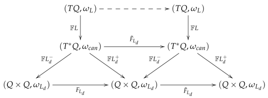
The two discrete fiber derivatives $\mathbb{F}{L}_d^{\pm }$ induce a single unique discrete symplectic form ${\omega }_{L_d}={\omega }_{L_d}^{\pm }={\left(\mathbb{F}{L}_d^{\pm }\right)}^{\ast }{\omega }_{can}$ on $Q\times Q$,

$${\omega }_{L_d}(q_k,q_{k+1})=\frac{{\partial }^2{L}_d}{\partial q_k\partial q_{k+1}}(q_k,q_{k+1})d{q}_k\wedge d{q}_{k+1},$$

(28)

and the discrete Lagrangian map is symplectic with respect to ${\omega }_{L_d}$ on $Q\times Q$, i.e., $F_{L_d}^{\ast }{\omega }_{L_d}={\omega }_{L_d}$.

The discrete Lagrangian and Hamiltonian maps can be expressed in terms of the discrete fiber derivatives, $F_{L_d}=\mathbb{F}{L}_d^{+}\circ {(\mathbb{F}{L}_d^{-})}^{-1}$, and ${\tilde{F}}_{L_d}={(\mathbb{F}{L}_d^{-})}^{-1}\circ \mathbb{F}{L}_d^{+}$, respectively. This characterization of the discrete flow maps underlies the proof of the variational error analysis theorem.

These properties may be summarized in the following commutative diagram,

If the exact discrete Lagrangian $L_d^E$ is used, then the discrete Hamiltonian map ${\tilde{F}}_{L_d}$ is equal to the time-h flow map of Hamilton’s equations, and the dotted arrow is the time-h flow map of the Euler–Lagrange equations.

The variational integrator approach to constructing symplectic integrators simplifies the numerical analysis of these methods. In particular, the task of establishing the geometric conservation properties and order of accuracy of the discrete Lagrangian map $F_{L_d}$ reduces to the simpler task of verifying certain properties of the discrete Lagrangian instead.

3.3. Discrete Hamilton–Jacobi Formulation

In the context of discrete variational mechanics, discrete Hamilton–Jacobi theory can be viewed as a composition theorem which relates the composition of symplectic maps generated by a Type II generating function $H_d^{+}(q_k,p_{k+1})$ with a symplectic map generated by a Type I generating function $S_d^k(q_0,q_k)$. By convention, the first argument $q_0$ in the composition generating function is typically omitted, and we simply consider it to be a function $S_d^k\left(q_k\right)$ of the final position $q_k$.

The right discrete Hamiltonian, $H_d^{+}(q_k,p_{k+1})$ [12], is related to the discrete Lagrangian by the Legendre transform,

$$H_d^{+}(q_k,p_{k+1})=⟨p_{k+1},q_{k+1}⟩-L_d(q_k,q_{k+1}),$$

where we impose the condition that $p_{k+1}=D_2{L}_d(q_k,q_{k+1})$. Equivalently, this can be characterized variationally by $H_d^{+}(q_k,p_{k+1})={ext}_{p_k}[⟨p_{k+1},q_{k+1}⟩-L_d(q_k,q_{k+1})]$. This leads to a discrete Hamilton’s principle in phase space,

$$\delta \sum _{i=0}^{n-1}\left\{⟨p_{i+1},q_{i+1}⟩-H_d^{+}(q_i,p_{i+1})\right\}=0,$$

which yields the right discrete Hamilton’s equations,

$$q_{k+1}=D_2{H}_d^{+}(q_k,p_{k+1}),p_k=D_1{H}_d^{+}(q_k,p_{k+1}),$$

(29)

which is precisely the characterization of a symplectic map in terms of Type II generating function.

The continuous Hamilton–Jacobi equation can be derived by considering the evolution properties of Jacobi’s solution, which is the action integral evaluated along the solution of the Euler–Lagrange equations. One can derive a discrete Hamilton–Jacobi theory by considering a discrete analogue of Jacobi’s solution, expressed in terms of the right discrete Hamiltonian,

$$S_d^k\left(q_k\right)\equiv \sum _{i=0}^{k-1}\left\{p_{i+1}·q_{i+1}-H_d^{+}(q_i,p_{i+1})\right\},$$

which we evaluate along a solution of the right discrete Hamilton’s equations (29). From this, we have,

$$S_d^{k+1}\left(q_{k+1}\right)-S_d^k\left(q_k\right)=p_{k+1}·q_{k+1}-H_d^{+}(q_k,p_{k+1}),$$

(30)

where $p_{k+1}$ is considered to be a function of $q_k$ and $q_{k+1}$. Taking derivatives with respect to $q_{k+1}$, we obtain,

$$D{S}_d^{k+1}\left(q_{k+1}\right)=p_{k+1}+\frac{\partial p_{k+1}}{\partial q_{k+1}}·\left[q_{k+1}-D_2{H}_d^{+}(q_k,p_{k+1})\right],$$

but the term inside the parenthesis vanishes as we are restricting this to a solution of the right discrete Hamilton’s equations. Therefore, we have that

$$D{S}_d^{k+1}\left(q_{k+1}\right)=p_{k+1},$$

which when substituted into (30) yields the discrete Hamilton–Jacobi equation,

$$S_d^{k+1}\left(q_{k+1}\right)-S_d^k\left(q_k\right)=D{S}_d^{k+1}\left(q_{k+1}\right)·q_{k+1}-H_d^{+}(q_k,D{S}_d^{k+1}\left(q_{k+1}\right)).$$

3.4. Discrete Hamilton–Pontryagin Principle

Leok and Ohsawa [13] considered the discrete Hamilton’s principle and relaxed the discrete second-order condition,

$$q_k^1=q_{k+1}^0,$$

and reimposed it using Lagrange multipliers $p_{k+1}$, in order to derive the discrete Hamilton–Pontryagin principle on $(Q\times Q){\times }_Q{T}^{\ast }Q$,

$$\delta \left[{\sum }_{i=0}^{n-1}{L}_d(q_i^0,q_i^1)+{\sum }_{i=0}^{n-2}{p}_{i+1}(q_{i+1}^0-q_i^1)\right]=0.$$

(31)

Here, the superscripts 0, or 1 on $q_i$ refers to the first or second slot, respectively, in $Q\times Q$. This in turn yields the implicit discrete Euler–Lagrange equations,

$$q_k^1=q_{k+1}^0,p_{k+1}=D_2{L}_d(q_k^0,q_k^1),p_k=-D_1{L}_d(q_k^0,q_k^1),$$

(32)

where $D_1,D_2$ denote as before the partial derivative with respect to the first or second argument in $L_d$. Making the identification $q_k=q_k^0=q_{k-1}^1$, the last two equations define the discrete fiber derivatives, $\mathbb{F}{L}_d^{\pm }:Q\times Q\to T^{\ast }Q$ as given by (23) and (24). Discrete fiber derivatives induce a discrete symplectic form, ${\omega }_{L_d}\equiv {(\mathbb{F}{L}_d^{\pm })}^{\ast }{\omega }_{can}$, and the discrete Lagrangian map $F_{L_d}\equiv {(\mathbb{F}{L}_d^{-})}^{-1}\circ \mathbb{F}{L}_d^{+}:(q_{k-1},q_k)\mapsto (q_k,q_{k+1})$ and the discrete Hamiltonian map ${\tilde{F}}_{L_d}\equiv \mathbb{F}{L}_d^{+}\circ {(\mathbb{F}{L}_d^{-})}^{-1}:(q_k,p_k)\mapsto (q_{k+1},p_{k+1})$ preserve ${\omega }_{L_d}$ and ${\omega }_{can}$, respectively.

4. Information Geometry

4.1. Statistical Structure on $\mathbb{M}$

On a differentiable manifold $\mathbb{M}$ endowed with a metric g and a torsion-free affine connection ∇, the compatibility of a metric g and a connection ∇ is encoded by the cubic form 3-tensor field $C=\nabla g$, i.e., the covariant derivative of g. In a local coordinate system with basis ${\partial }_i\equiv \partial /\partial x^i$, the metric tensor g is locally represented by

$$g_{ij}\left(x\right)=g({\partial }_i,{\partial }_j),$$

(33)

and the components of ∇ takes the contravariant form ${\Gamma }_{ij}^l$, where

$${\nabla }_{{\partial }_i}{\partial }_j=\sum _l{\Gamma }_{ij}^l{\partial }_l,$$

(34)

or the covariant form ${\Gamma }_{ij,k}$, where

$${\Gamma }_{ij,k}=g({\nabla }_{{\partial }_i}{\partial }_j,{\partial }_k)=\sum _l{g}_{lk}{\Gamma }_{ij}^l.$$

(35)

Torsion-freeness of ∇ implies the symmetry of its (first) two lower indices, i.e.,

$${\Gamma }_{ij}^l\left(x\right)={\Gamma }_{ji}^l\left(x\right),{\Gamma }_{ij,l}\left(x\right)={\Gamma }_{ji,l}\left(x\right).$$

We can now compute the cubic form,

$$C({\partial }_i,{\partial }_j,{\partial }_k)=\left({\nabla }_{{\partial }_k}g\right)({\partial }_i,{\partial }_j)={\partial }_{k}g({\partial }_i,{\partial }_j)-g({\nabla }_{{\partial }_k}{\partial }_i,{\partial }_j)-g({\partial }_i,{\nabla }_{{\partial }_k}{\partial }_j),$$

or in components,

$$C_{ijk}=\frac{\partial g_{ij}}{\partial x_k}-{\Gamma }_{ki,j}-{\Gamma }_{kj,i}.$$

(36)

When the cubic form is identically zero, ∇ is said to be parallel with respect to g. A torsion-free connection parallel to g is called the Levi-Civita connection $\widehat{\nabla }$ associated to the given metric g:

$${\partial }_{k}g({\partial }_i,{\partial }_j)=g({\widehat{\nabla }}_{{\partial }_k}{\partial }_i,{\partial }_j)+g({\partial }_i,{\widehat{\nabla }}_{{\partial }_k}{\partial }_j).$$

(37)

The fundamental theorem of Riemannian geometry establishes the existence and uniqueness of the Levi-Civita connection, which is a solution of (37), and is given by,

$${\widehat{\Gamma }}_{ij}^k=\sum _l\frac{g^{kl}}{2}\left(\frac{\partial g_{il}}{\partial x^j}+\frac{\partial g_{jl}}{\partial x^i}-\frac{\partial g_{ij}}{\partial x^l}\right).$$

Generalizing the notion of parallelism of a connection is the notion of conjugacy (denoted by ∗) between two connections. A connection ${\nabla }^{\ast }$ is said to be conjugate (or dual) to ∇ with respect to g if

$${\partial }_{k}g({\partial }_i,{\partial }_j)=g({\nabla }_{{\partial }_k}{\partial }_i,{\partial }_j)+g({\partial }_i,{\nabla }_{{\partial }_k}^{\ast }\partial j).$$

(38)

Clearly, ${\left({\nabla }^{\ast }\right)}^{\ast }=\nabla$. Moreover, $\widehat{\nabla }$, which satisfies (37), is special in the sense that it is self-conjugate ${(\widehat{\nabla })}^{\ast }=\widehat{\nabla }$. Writing out (38):

$$\frac{\partial g_{ij}}{\partial x^k}={\Gamma }_{ki,j}+{\Gamma }_{kj,i}^{\ast },$$

(39)

where ${\Gamma }_{kj,i}^{\ast }$ is defined analogously to (34) and (35),

$${\nabla }_{{\partial }_i}^{\ast }{\partial }_j=\sum _l{\Gamma }_{ij}^{\ast l}{\partial }_l,$$

so that

$${\Gamma }_{kj,i}^{\ast }=g({\nabla }_{{\partial }_j}^{\ast }{\partial }_k,{\partial }_i)=\sum _l{g}_{il}{\Gamma }_{kj}^{\ast l}.$$

From (36) and (38), the cubic form can now be written as

$$C_{ijk}={\Gamma }_{kj,i}^{\ast }-{\Gamma }_{kj,i}.$$

Clearly, $C_{ijk}=C_{jik}$, i.e., it is symmetric with respective to its first two indices. When both ∇ and ${\nabla }^{\ast }$ are torsion-free, this implies that

$${\Gamma }_{kj,i}={\Gamma }_{jk,i},{\Gamma }_{kj,i}^{\ast }={\Gamma }_{jk,i}^{\ast },$$

then $C_{ijk}=C_{ikj}$, which leads to C being totally symmetric in all the indices,

$$C_{ijk}=C_{ikj}=C_{kij}=C_{kji}=C_{jki}=C_{jik}.$$

Requiring that $C_{ijk}$ is totally symmetric imposes a compatibility condition between g and ∇, so that they form a Codazzi pair (see [14]), which generalizes the Levi-Civita coupling (whose corresponding cubic form $C_{ijk}\equiv 0$). Lauritzen [15] defined a statistical manifold $(\mathbb{M},g,\nabla )$ to be a manifold $\mathbb{M}$ equipped with metric g and connection ∇ such that (i) ∇ is torsion-free; (ii) $\nabla g\equiv C$ is totally symmetric. Equivalently, a manifold has a statistical structure when the conjugate (with respect to g) ${\nabla }^{\ast }$ of a torsion-free connection ∇ is also torsion-free. In this case, ${\nabla }^{\ast }g=-C$, and the Levi-Civita connection $\widehat{\nabla }=(\nabla +{\nabla }^{\ast })/2$.

On a statistical manifold, one can define a one-parameter family of affine connections ${\nabla }^{\left(\alpha \right)}$, called $\alpha$-connections ($\alpha \in \mathbb{R}$) [2]:

$${\nabla }^{\left(\alpha \right)}=\frac{1+\alpha }{2}\nabla +\frac{1-\alpha }{2}{\nabla }^{\ast }.$$

(40)

Obviously, ${\nabla }^{\left(0\right)}=\widehat{\nabla }$ is the Levi-Civita connection, and the cubic form is given by ${\nabla }^{\left(\alpha \right)}g=\alpha C$.

The curvature/flatness of a connection ∇ is described by the Riemann curvature tensor R, defined as

$$R({\partial }_i,{\partial }_j){\partial }_k=({\nabla }_{{\partial }_i}{\nabla }_{{\partial }_j}-{\nabla }_{{\partial }_j}{\nabla }_{{\partial }_i}){\partial }_k.$$

Writing $R({\partial }_i,{\partial }_j){\partial }_k={\sum }_l{R}_{kij}^l{\partial }_l$ and substituting (34), the components of the Riemann curvature tensor are

$$R_{kij}^l\left(x\right)=\frac{\partial {\Gamma }_{jk}^l\left(x\right)}{\partial x^i}-\frac{\partial {\Gamma }_{ik}^l\left(x\right)}{\partial x^j}+\sum _m{\Gamma }_{im}^l\left(x\right){\Gamma }_{jk}^m\left(x\right)-\sum _m{\Gamma }_{jm}^l\left(x\right){\Gamma }_{ik}^m\left(x\right).$$

By definition, $R_{kij}^l$ is antisymmetric when $i\leftrightarrow j$. The covariant form of the Riemann curvature is

$$R_{lkij}=\sum _m{g}_{lm}{R}_{kij}^m.$$

When the connection is torsion-free, $R_{lkij}$ is antisymmetric when $i\leftrightarrow j$ or when $k\leftrightarrow l$, and symmetric when $(i,j)\leftrightarrow (l,k)$. It is related to the Ricci tensor Ric by ${Ric}_{kj}={\sum }_{i,l}{R}_{lkij}{g}^{il}$.

In addition, it can be shown that the curvatures $R_{lkij},R_{lkij}^{\ast }$ for the pair of conjugate connections $\nabla ,{\nabla }^{\ast }$ satisfy

$$R_{lkij}=R_{lkij}^{\ast }.$$

A connection is said to be flat when $R_{kij}^l\left(x\right)\equiv 0$. So, ∇ is flat if and only if ${\nabla }^{\ast }$ is flat. In this case, the manifold is said to be dually-flat, and the metric g takes on a particular form (to be discussed later).

4.2. Divergence Function and Induced Geometry

A divergence function $\mathcal{D}:\mathbb{M}\times \mathbb{M}\to {\mathbb{R}}_{\ge 0}$ on a manifold $\mathbb{M}$ with respect to a local chart $V\subseteq {\mathbb{R}}^n$ is a $C^3$ function satisfying

(i)

$\mathcal{D}(x,y)\ge 0,\forall x,y\in V$, with equality holding if and only if $x=y$;

(ii)

${\mathcal{D}}_i(x,x)={\mathcal{D}}_{,j}(x,x)=0,\forall i,j\in \{1,2,\cdots ,n\}$;

(iii)

$-{\mathcal{D}}_{i,j}(x,x)$ is positive-definite.

Here ${\mathcal{D}}_i(x,y)={\partial }_{x^i}D(x,y)$, ${\mathcal{D}}_{,i}(x,y)={\partial }_{y^i}\mathcal{D}(x,y)$ denote partial derivatives with respect to the i-th component of point x and of point y, respectively, and ${\mathcal{D}}_{i,j}(x,y)={\partial }_{x^i}{\partial }_{y^j}\mathcal{D}(x,y)$ the second-order mixed derivative, and so on.

On a manifold, divergence functions act as pseudo-distance functions that are nonnegative but need not be symmetric. Every divergence function induces a dualistic Riemannian structure, i.e., statistical structure, which was first demonstrated by Eguchi (see [16]).

Lemma 1.

A divergence function induces a Riemannian metric g and a pair of torsion-free conjugate connections $\nabla ,{\nabla }^{\ast }$ given as

$$\begin{array}{cc}\hfill g_{ij}\left(x\right)& =-{\left.{\mathcal{D}}_{i,j}(x,y)\right|}_{x=y},\hfill \\ \hfill {\Gamma }_{ij,k}\left(x\right)& =-{\left.{\mathcal{D}}_{ij,k}(x,y)\right|}_{x=y},\hfill \\ \hfill {\Gamma }_{ij,k}^{\ast }\left(x\right)& =-{\left.{\mathcal{D}}_{k,ij}(x,y)\right|}_{x=y}.\hfill \end{array}$$

The ${\Gamma }_{ij,k},{\Gamma }_{ij,k}^{\ast }$ are torsion-free and are conjugate with respect to the induced metric $g_{ij}$. Hence, the divergence function $\mathcal{D}$ induces $(\mathbb{M},g,\nabla ,{\nabla }^{\ast })$, which is a statistical manifold (Lauritzen [15]).

A popular divergence function is the Bregman divergence ${\mathcal{B}}_{\mathsf{\Phi }}(x,y)$ [17], which is associated to a strictly convex function $\mathsf{\Phi }$:

$${\mathcal{B}}_{\mathsf{\Phi }}(x,y)=\mathsf{\Phi }\left(y\right)-\mathsf{\Phi }\left(x\right)-⟨y-x,\partial \mathsf{\Phi }\left(x\right)⟩,$$

(41)

where $\partial \mathsf{\Phi }=[{\partial }_1\mathsf{\Phi },\cdots ,{\partial }_n\mathsf{\Phi }]$ denotes the exterior derivative, and ${⟨·,·⟩}_n$ denotes the canonical pairing of a vector $x=[x^1,\cdots ,x^n]\in {\mathbb{R}}^n$ and a covector $u=[u_1,\cdots ,u_n]\in {\tilde{\mathbb{R}}}_n$ (dual to ${\mathbb{R}}^n$), i.e.,

$$⟨x,u⟩=\sum _{i=1}^n{x}^i{u}_i.$$

(42)

Where there is no danger of confusion, the subscript n in ${⟨·,·⟩}_n$ is often omitted. A basic fact in convex analysis is that the necessary and sufficient condition for a smooth function $\mathsf{\Phi }$ to be strictly convex is

$${\mathcal{B}}_{\mathsf{\Phi }}(x,y)>0,$$

(43)

for all $x\ne y$.

Recall that when $\mathsf{\Phi }$ is convex, its convex conjugate, $\tilde{\mathsf{\Phi }}:\tilde{V}\subseteq {\tilde{\mathbb{R}}}_n\to \mathbb{R}$, is defined through the Legendre transform:

$$\tilde{\mathsf{\Phi }}(u)=⟨{(\partial \mathsf{\Phi })}^{-1}(u),u⟩-\mathsf{\Phi }({(\partial \mathsf{\Phi })}^{-1}(u)),$$

(44)

with $\widetilde{\tilde{\mathsf{\Phi }}}=\mathsf{\Phi }$ and $(\partial \mathsf{\Phi })={(\partial \tilde{\mathsf{\Phi }})}^{-1}$. Since $\tilde{\mathsf{\Phi }}$ is also convex, by (43), we obtain the Fenchel inequality,

$$\mathsf{\Phi }\left(x\right)+\tilde{\mathsf{\Phi }}\left(u\right)-⟨x,u⟩\ge 0,$$

for any $x\in V$, $u\in \tilde{V}$, with equality holding if and only if

$$u=(\partial \mathsf{\Phi })(x)={(\partial \tilde{\mathsf{\Phi }})}^{-1}(x)⟷x=(\partial \tilde{\mathsf{\Phi }})(u)={(\partial \mathsf{\Phi })}^{-1}(u),$$

(45)

or, in component form,

$$u_i=\frac{\partial \mathsf{\Phi }}{\partial x^i}⟷x^i=\frac{\partial \tilde{\mathsf{\Phi }}}{\partial u_i}.$$

(46)

Using conjugate variables, we can introduce the canonical divergence ${\mathcal{A}}_{\mathsf{\Phi }}:V\times \tilde{V}\to {\mathbb{R}}_{+}$ (and ${\mathcal{A}}_{\tilde{\mathsf{\Phi }}}:\tilde{V}\times V\to {\mathbb{R}}_{+}$),

$${\mathcal{A}}_{\mathsf{\Phi }}(x,v)=\mathsf{\Phi }\left(x\right)+\tilde{\mathsf{\Phi }}\left(v\right)-⟨x,v⟩={\mathcal{A}}_{\tilde{\mathsf{\Phi }}}(v,x).$$

They are related to the Bregman divergence (41) via the relation

$${\mathcal{B}}_{\mathsf{\Phi }}(x,{(\partial \mathsf{\Phi })}^{-1}(v))={\mathcal{A}}_{\mathsf{\Phi }}(x,v)={\mathcal{B}}_{\tilde{\mathsf{\Phi }}}((\partial \tilde{\mathsf{\Phi }})(x),v).$$

Though the Bregman divergence is not a metric, it satisfies a quadrilateral relation [18]: For any four points $x,x^{\prime },x^{″},x^{‴}\in V$,

$${\mathcal{B}}_{\mathsf{\Phi }}(x,x^{\prime })+{\mathcal{B}}_{\mathsf{\Phi }}(x^{‴},x^{″})-{\mathcal{B}}_{\mathsf{\Phi }}(x,x^{″})-{\mathcal{B}}_{\mathsf{\Phi }}(x^{‴},x^{\prime })=⟨x^{″}-x^{\prime },\partial \mathsf{\Phi }\left(x\right)-\partial \mathsf{\Phi }\left(x^{‴}\right)⟩.$$

As a special case, when $x^{‴}=x^{\prime }$, ${\mathcal{B}}_{\mathsf{\Phi }}(x^{‴},x^{\prime })=0$, the above equality reduces to the Pythagorean (generalized cosine) relation among three points $x,x^{\prime },x^{″}\in V$:

$${\mathcal{B}}_{\mathsf{\Phi }}(x,x^{\prime })+{\mathcal{B}}_{\mathsf{\Phi }}(x^{\prime },x^{″})-{\mathcal{B}}_{\mathsf{\Phi }}(x,x^{″})=⟨x^{″}-x^{\prime },\partial \mathsf{\Phi }\left(x\right)-\partial \mathsf{\Phi }\left(x^{\prime }\right)⟩.$$

This is the Pythagorean relation [3] for a dually-flat space. Using this relation, one can state minimization problems for divergence functions.

The quadrilateral relation can be expressed in terms of the canonical divergence $\mathcal{A}$ as follows,

$${\mathcal{A}}_{\mathsf{\Phi }}(x,u)+{\mathcal{A}}_{\mathsf{\Phi }}(y,v)-{\mathcal{A}}_{\mathsf{\Phi }}(x,v)-{\mathcal{A}}_{\mathsf{\Phi }}(y,u)=⟨x-y,v-u⟩,$$

for any four points $x,y\in V$, $v,u\in \tilde{V}$.

Zhang [5] introduced the $\alpha$-indexed family of $\mathsf{\Phi }$-divergence functions ${\mathcal{D}}_{\mathsf{\Phi }}^{\left(\alpha \right)}$ on $V\times V$,

$${\mathcal{D}}_{\mathsf{\Phi }}^{\left(\alpha \right)}(x,y)=\frac{4}{1-{\alpha }^2}\left(\frac{1-\alpha }{2}\mathsf{\Phi }\left(x\right)+\frac{1+\alpha }{2}\mathsf{\Phi }\left(y\right)-\mathsf{\Phi }\left(\frac{1-\alpha }{2}x+\frac{1+\alpha }{2}y\right)\right).$$

(47)

Furthermore, ${\mathcal{D}}_{\mathsf{\Phi }}^{(\pm 1)}(x,y)$ is defined by taking ${lim}_{\alpha \to \pm 1}$:

$$\begin{array}{cc}\hfill {\mathcal{D}}_{\mathsf{\Phi }}^{(-1)}(x,y)& ={\mathcal{D}}_{\mathsf{\Phi }}^{\left(1\right)}(y,x)={\mathcal{B}}_{\mathsf{\Phi }}(x,y),\hfill \\ \hfill {\mathcal{D}}_{\mathsf{\Phi }}^{\left(1\right)}(x,y)& ={\mathcal{D}}_{\mathsf{\Phi }}^{(-1)}(y,x)={\mathcal{B}}_{\mathsf{\Phi }}(y,x).\hfill \end{array}$$

Note that ${\mathcal{D}}_{\mathsf{\Phi }}^{\left(\alpha \right)}(x,y)$ satisfies the relation (called referential duality in [5,19]),

$${\mathcal{D}}_{\mathsf{\Phi }}^{\left(\alpha \right)}(x,y)={\mathcal{D}}_{\mathsf{\Phi }}^{(-\alpha )}(y,x),$$

that is, exchanging the two points in the directed distance amounts to $\alpha \leftrightarrow -\alpha$.

4.3. Hessian Manifolds and Biorthogonal Coordinates

Applying Lemma 1 to the Bregman divergence ${\mathcal{B}}_{\mathsf{\Phi }}$ induces the following metric,

$$g_{ij}\left(x\right)=\frac{{\partial }^2\mathsf{\Phi }\left(x\right)}{\partial x^i\partial x^j},$$

and the pair of torsion-free conjugate connections,

$${\Gamma }_{ij,k}\left(x\right)=0,{\Gamma }_{ij,k}^{\ast }\left(x\right)=\frac{{\partial }^3\mathsf{\Phi }\left(x\right)}{\partial x^i\partial x^j\partial x^k}.$$

In this case, $\mathbb{M}$ is dually-flat. This yields a Hessian manifold, where g takes the form of the Hessian of a strictly convex function $\mathsf{\Phi }$. More generally, as shown in [5], the $\mathsf{\Phi }$-divergence ${\mathcal{D}}_{\mathsf{\Phi }}^{\left(\alpha \right)}$ of (47), which degenerates to the Bregman divergence ${\mathcal{B}}_{\mathsf{\Phi }}$ when $\alpha =\pm 1$, induces an $\alpha$-independent Hessian metric $g_{ij}$ along with the following $\alpha$-connections

$${\Gamma }_{ij,k}^{\left(\alpha \right)}\left(x\right)=\frac{1-\alpha }{2}\frac{{\partial }^3\mathsf{\Phi }\left(x\right)}{\partial x^i\partial x^j\partial x^k},{\Gamma }_{ij,k}^{\left(\alpha \right)\ast }\left(x\right)=\frac{1+\alpha }{2}\frac{{\partial }^3\mathsf{\Phi }\left(x\right)}{\partial x^i\partial x^j\partial x^k}.$$

Hessian manifolds enjoy a special status in information geometry, as they exhibit biorthogonal coordinates on $\mathbb{M}$ that are globally affine coordinates despite the nontrivial Riemannian (Hessian) metric on $\mathbb{M}$.

Consider the coordinate transform $x\mapsto u$,

$${\partial }^i\equiv \frac{\partial }{\partial u_i}=\sum _l\frac{\partial x^l}{\partial u_i}\frac{\partial }{\partial x^l}=\sum _l{F}^{li}{\partial }_l,$$

where the Jacobian matrix F is given by

$$F_{ij}\left(x\right)=\frac{\partial u_i}{\partial x^j},F^{ij}\left(u\right)=\frac{\partial x^i}{\partial u_j},\sum _l{F}_{il}{F}^{lj}={\delta }_j^i,$$

(48)

where ${\delta }_j^i$ is the Kronecker delta, which takes the value 1 when $i=j$ and 0 otherwise. If the new coordinate system $u=[u_1,\cdots ,u_n]$ (with components denoted by subscripts) is such that

$$F_{ij}\left(x\right)=g_{ij}\left(x\right),$$

(49)

then the x-coordinate system and the u-coordinate system are said to be biorthogonal to each other, since, from the definition of the metric tensor (33),

$$g({\partial }_i,{\partial }^j)=g({\partial }_i,\sum _l{F}^{lj}{\partial }_l)=\sum _l{F}^{lj}g({\partial }_i,{\partial }_l)=\sum _l{F}^{lj}{g}_{il}={\delta }_i^j.$$

In this case, we define

$$g^{ij}\left(u\right)=g({\partial }^i,{\partial }^j),$$

(50)

which is equal to $F^{ij}$, the Jacobian of the inverse coordinate transform $u\mapsto x$. We also introduce the contravariant representation of the affine connection ∇ with respect to the u-coordinate system, and denote it by an unconventional notation ${\Gamma }_t^{rs}$, which is defined by

$${\nabla }_{{\partial }^r}{\partial }^s=\sum _t{\Gamma }_t^{rs}{\partial }^t;$$

similarly, ${\Gamma }_t^{\ast rs}$ is defined by

$${\nabla }_{{\partial }^r}^{\ast }{\partial }^s=\sum _t{\Gamma }_t^{\ast rs}{\partial }^t.$$

The covariant representation of the affine connections will be denoted by superscripted $\Gamma$ and ${\Gamma }^{\ast }$,

$${\Gamma }^{ij,k}\left(u\right)=g({\nabla }_{{\partial }^i}{\partial }^j,{\partial }^k),{\Gamma }^{\ast ij,k}\left(u\right)=g({\nabla }_{{\partial }^i}^{\ast }{\partial }^j,{\partial }^k).$$

(51)

The representation of the affine connections in the u-coordinate system (denoted by superscripts) and the x-coordinate system (denoted by subscripts) are related by

$${\Gamma }_t^{rs}\left(u\right)=\sum _k\left(\sum _{i,j}\frac{\partial x^r}{\partial u_i}\frac{\partial x^s}{\partial u_j}{\Gamma }_{ij}^k\left(x\right)+\frac{{\partial }^2{x}^k}{\partial u_r\partial u_s}\right)\frac{\partial u_k}{\partial x^t},$$

(52)

and

$${\Gamma }^{rs,t}\left(u\right)=\sum _{i,j,k}\frac{\partial x^r}{\partial u_i}\frac{\partial x^s}{\partial u_j}\frac{\partial x^t}{\partial u_k}{\Gamma }_{ij,k}\left(x\right)+\frac{{\partial }^2{x}^t}{\partial u_r\partial u_s}.$$

(53)

Similarly relations hold between ${\Gamma }_t^{\ast rs}\left(u\right)$ and ${\Gamma }_{ij}^{\ast k}\left(x\right)$, and between ${\Gamma }^{\ast rs,t}\left(u\right)$ and ${\Gamma }_{ij,k}^{\ast }\left(x\right)$.

Analogous to (39), we have the following identity,

$$\frac{{\partial }^2{x}^t}{\partial u_s\partial u_r}=\frac{\partial g^{rt}\left(u\right)}{\partial u_s}={\Gamma }^{rs,t}\left(u\right)+{\Gamma }^{\ast ts,r}\left(u\right).$$

Therefore, with respect to biorthogonal coordinates, a pair of conjugate connections $\nabla ,{\nabla }^{\ast }$ satisfy,

$${\Gamma }^{\ast ts,r}\left(u\right)=-\sum _{i,j,k}{g}^{ir}\left(u\right)g^{js}\left(u\right)g^{kt}\left(u\right){\Gamma }_{ij,k}\left(x\right),$$

(54)

and

$${\Gamma }_r^{\ast ts}\left(u\right)=-\sum _j{g}^{js}\left(u\right){\Gamma }_{jr}^t\left(x\right).$$

(55)

We now investigate conditions for the existence of biorthogonal coordinates on a Riemannian manifold $(\mathbb{M},g)$. From its definition (49), it can easily be shown that

Proposition 1

([20]). A Riemannian manifold $\mathbb{M}$ with metric $g_{ij}$ admits biorthogonal coordinates if and only if $\frac{\partial g_{ij}}{\partial x^k}$ is totally symmetric, i.e.,

$$\frac{\partial g_{ij}\left(x\right)}{\partial x^k}=\frac{\partial g_{ik}\left(x\right)}{\partial x^j}.$$

(56)

In this case, $\mathbb{M}$ is Hessian.

That (56) is satisfied for biorthogonal coordinates is evident by virtue of (48) and (49). Conversely, given (56), there must be n functions $u_i\left(x\right),i=1,2,\cdots ,n$, such that,

$$\frac{\partial u_i\left(x\right)}{\partial x^j}=g_{ij}\left(x\right)=g_{ji}\left(x\right)=\frac{\partial u_j\left(x\right)}{\partial x^i}.$$

The above identity implies that there exist a function $\mathsf{\Phi }$ such that $u_i={\partial }_i\mathsf{\Phi }$ and, by positive definiteness of $g_{ij}$, $\mathsf{\Phi }$ would have to be a strictly convex function! In this case, the x- and u-variables satisfy (45), and the pair of convex functions, $\mathsf{\Phi }$ and its conjugate $\tilde{\mathsf{\Phi }}$, are related to $g_{ij}$ and $g^{ij}$ by

$$g_{ij}\left(x\right)=\frac{{\partial }^2\mathsf{\Phi }\left(x\right)}{\partial x^i\partial x^j}⟷g^{ij}\left(u\right)=\frac{{\partial }^2\tilde{\mathsf{\Phi }}\left(u\right)}{\partial u_i\partial u_j}.$$

It follows from Proposition 1 that a necessary and sufficient condition for a Riemannian manifold to admit biorthogonal coordinates it that its Levi-Civita connection is given by

$${\widehat{\Gamma }}_{ij,k}\left(x\right)\equiv \frac{1}{2}\left(\frac{\partial g_{ik}}{\partial x^j}+\frac{\partial g_{jk}}{\partial x^i}-\frac{\partial g_{ij}}{\partial x^k}\right)=\frac{1}{2}\frac{\partial g_{ij}}{\partial x^k}.$$

From this, the following can be shown:

Corollary 1.

A Riemannian manifold $(\mathbb{M},g)$ admits a pair of biorthogonal coordinates x and u if and only if there exists a pair of conjugate connections ∇ and ${\nabla }^{\ast }$ such that ${\Gamma }_{ij,k}\left(x\right)=0,{\Gamma }^{\ast rs,t}\left(u\right)=0$.

In other words, biorthogonal coordinates are affine coordinates for the dually-flat pair of connections. In fact, we can now define a pair of torsion-free connections by

$${\Gamma }_{ij,k}\left(x\right)=0,{\Gamma }_{ij,k}^{\ast }\left(x\right)=\frac{\partial g_{ij}}{\partial x^k},$$

and show that they are conjugate with respect to g, that is, they satisfy (38). This means that we select an affine connection ∇ such that x is its affine coordinate system. From (53), when ${\nabla }^{\ast }$ is expressed in u-coordinates,

$$\begin{array}{cc}\hfill {\Gamma }^{\ast rs,t}\left(u\right)& ={\displaystyle \sum _{i,j,k}}{g}^{ir}\left(u\right)g^{js}\left(u\right)\frac{\partial x^k}{\partial u_t}\frac{\partial g_{ij}\left(x\right)}{\partial x^k}+\frac{\partial g^{ts}\left(u\right)}{\partial u_r}\hfill \\ & ={\displaystyle \sum _{i,j}}{g}^{ir}\left(u\right)\left(-\frac{\partial g^{js}\left(u\right)}{\partial u_t}{g}_{ij}\left(x\right)\right)+\frac{\partial g^{ts}\left(u\right)}{\partial u_r}\hfill \\ & =-{\displaystyle \sum _j}{\delta }_j^r\frac{\partial g^{js}\left(u\right)}{\partial u_t}+\frac{\partial g^{ts}\left(u\right)}{\partial u_r}=0.\hfill \end{array}$$

This implies that u is an affine coordinate system with respect to ${\nabla }^{\ast }$. Furthermore,

$$g^{ij}\left(u\right)=\frac{{\partial }^2\tilde{\mathsf{\Phi }}\left(u\right)}{\partial u_i\partial u_j},{\Gamma }^{ij,k}\left(u\right)=\frac{{\partial }^3\tilde{\mathsf{\Phi }}\left(u\right)}{\partial u_i\partial u_j\partial u_k},$$

where $\tilde{\mathsf{\Phi }}$ is the convex conjugate of $\mathsf{\Phi }$. Therefore, biorthogonal coordinates are affine coordinates for a pair of dually-flat connections. On the manifold of parameterized probability density functions, if the x-coordinates are the natural parameters, then the u-coordinates are the expectations.

5. Linking Information Geometry with Geometric Mechanics

5.1. Symplectic Structure on $Q\times Q$ Induced from the Divergence Function $\mathcal{D}$

We will now establish the connection between information geometry and discrete geometric mechanics. The divergence function from information geometry can be viewed as a Type I generating function of a symplectic map, and in particular, it can be viewed as a discrete Lagrangian in the sense of discrete Lagrangian mechanics. More specifically, let the configuration manifold be the information manifold, i.e., $Q=\mathbb{M}$, and the discrete Lagrangian be the divergence function, i.e., $L_d=\mathcal{D}$. With this identification, we observe that the information geometric construction of symplectic structure on $\mathbb{M}\times \mathbb{M}$ described below is nothing but the discrete symplectic structure on $Q\times Q$ given in (28) where the discrete Lagrangian $L_d$ is replaced with the divergence function $\mathcal{D}$.

From information geometry, a divergence function $\mathcal{D}$ is given as a scalar-valued binary function on Q (of dimension n). We now view it as a unary function on $Q\times Q$ (of dimension $2n$) that vanishes along the diagonal ${\Delta }_Q\subset Q\times Q$. In this subsection, we investigate the conditions under which a divergence function can serve as a generating function of a symplectic structure on $Q\times Q$. A compatible metric on $Q\times Q$ will also be derived. When restricted to the diagonal submanifold ${\Delta }_Q$, the skew-symmetric symplectic form will vanish, so ${\Delta }_Q$, which carries a statistical structure, is actually a Lagrangian submanifold (see [21,22]).

First, we fix a point x in the first slot and a point y in the second slot of $(x,y)\in Q\times Q$ – this results in two n-dimensional submanifolds of $Q\times Q$ that will be denoted, $Q_x=Q\times \left\{y\right\}\simeq Q$ (with the y point fixed) and $Q_y=\left\{x\right\}\times Q\simeq Q$ (with the x point fixed), respectively. The canonical symplectic form ${\omega }_x$ on the cotangent bundle $T^{\ast }{Q}_x$ is given by

$${\omega }_x=\sum _{i}d{x}^i\wedge d{\xi }_i.$$

Given $\mathcal{D}$, we define a map $L_{\mathcal{D}}$ from $Q_y\subset Q\times Q$ to $T^{\ast }{Q}_x,(x,y)\mapsto (x,\xi )$, which is given by,

$$L_{\mathcal{D}}:(x,y)\mapsto (x,\sum _i{\mathcal{D}}_i(x,y)d{x}^i).$$

Recall that the comma in the subscript of a divergence function $\mathcal{D}$ indicates whether it is being differentiated with respect to a variable in the first or second slot. It is easily checked that there exists a neighborhood of the diagonal ${\Delta }_Q\subset Q\times Q$, such that the map $L_{\mathcal{D}}$ is a diffeomorphism. In particular, the Jacobian of the map is given by

$$\left(\begin{array}{cc}{\delta }_{ij}& {\mathcal{D}}_{ij}\\ 0& {\mathcal{D}}_{i,j}\end{array}\right),$$

which is nondegenerate in a neighborhood of the diagonal ${\Delta }_Q$.

We calculate the pullback by $L_{\mathcal{D}}$ of the canonical symplectic form ${\omega }_x$ on $T^{\ast }{Q}_x$ to $Q\times Q$:

$$\begin{array}{cc}\hfill L_{\mathcal{D}}^{\ast }{\omega }_x& =L_{\mathcal{D}}^{\ast }({\displaystyle \sum _i}d{x}^i\wedge d{\xi }_i)={\displaystyle \sum _i}d{x}^i\wedge d{\mathcal{D}}_i(x,y)\hfill \\ & ={\displaystyle \sum _i}d{x}^i\wedge {\displaystyle \sum _j}({\mathcal{D}}_{ij}(x,y)d{x}^j+{\mathcal{D}}_{i,j}d{y}^j)={\displaystyle \sum _{ij}}{\mathcal{D}}_{i,j}(x,y)d{x}^i\wedge d{y}^j.\hfill \end{array}$$

Here, ${\sum }_{ij}{\mathcal{D}}_{ij}d{x}^i\wedge d{x}^j=0$, since by the equality of mixed partials, ${\mathcal{D}}_{ij}(x,y)={\mathcal{D}}_{ji}(x,y)$ always holds.

Similarly, we consider the canonical symplectic form ${\omega }_y={\sum }_{i}d{y}^i\wedge d{\eta }_i$ on $T^{\ast }{Q}_y$ and define a map $R_{\mathcal{D}}$ from $Q\times Q\to T^{\ast }{Q}_y,(x,y)\mapsto (y,\eta )$, which is given by

$$R_{\mathcal{D}}:(x,y)=(y,\sum _i{\mathcal{D}}_{,i}(x,y)d{y}^i).$$

Using $R_{\mathcal{D}}$ to pullback ${\omega }_y$ to $Q\times Q$ yields an analogous formula:

$$R_{\mathcal{D}}^{\ast }{\omega }_y=-\sum _{ij}{\mathcal{D}}_{i,j}(x,y)d{x}^i\wedge d{y}^j.$$

Therefore, based on canonical symplectic forms on $T^{\ast }{Q}_x$ and $T^{\ast }{Q}_y$, we obtained the same symplectic form on $Q\times Q$

$${\omega }_{\mathcal{D}}(x,y)=-\sum _{ij}{\mathcal{D}}_{i,j}(x,y)d{x}^i\wedge d{y}^j.$$

(57)

Theorem 1

([22]). A divergence function $\mathcal{D}$ induces a symplectic form ${\omega }_{\mathcal{D}}$ (57) on $Q\times Q$ which is the pullback of the canonical symplectic forms ${\omega }_x$ and ${\omega }_y$ by the maps $L_{\mathcal{D}}$ and $R_{\mathcal{D}}$,

$$L_{\mathcal{D}}^{\ast }{\omega }_y=\sum _{ij}{\mathcal{D}}_{i,j}(x,y)d{x}^i\wedge d{y}^j=-R_{\mathcal{D}}^{\ast }{\omega }_x.$$

(58)

With the symplectic form ${\omega }_{\mathcal{D}}$ given as above, it is easy to check that ${\omega }_{\mathcal{D}}$ is closed:

$$d{\omega }_{\mathcal{D}}=\sum _{ijk}\left\{\frac{{\partial }^3\mathcal{D}}{\partial x^k\partial x^i\partial y^j}d{x}^k\wedge d{x}^i\wedge d{y}^j+\frac{{\partial }^3\mathcal{D}}{\partial y^k\partial x^i\partial y^j}d{y}^k\wedge d{x}^i\wedge d{y}^j\right\}=0.$$

It was Barndorff-Nielsen and Jupp [21] who first proposed (57) as an induced symplectic form on $Q\times Q$, apart from a minus sign; they called the divergence function $\mathcal{D}$ a york.

The fact that this symplectic structure coincides with the one introduced in discrete mechanics should come as no surprise. The $Q_x$ and $Q_y$ submanifolds are related to the two ways of viewing $Q\times Q$ as a bundle over Q, depending on whether one chooses ${\pi }_1:Q\times Q\to Q$, $(x,y)\mapsto x$ or ${\pi }_2:Q\times Q\to Q$, $(x,y)\mapsto y$ as the bundle projection. Then, the maps $L_{\mathcal{D}}$, $R_{\mathcal{D}}$ are, up to a sign, simply the discrete fiber derivatives $\mathbb{F}{L}_d^{\pm }$, where the discrete Lagrangian $L_d$ is replaced by the divergence function $\mathcal{D}$.

5.2. Divergence as a Type I Generating Function

As we have seen previously, symplectic maps are a natural way of describing the flow of Hamiltonian mechanics on the cotangent bundle $T^{\ast }Q$. We will now consider the characterization of symplectic maps in terms of generating functions, and in particular, we review three different parameterizations based on the classification given in Goldstein [23].

Lemma 2.

Given $(q_0,q_1)\in Q\times Q$, then $(q_0,p_0)\mapsto (q_1,p_1)$ on $T^{\ast }Q$ is symplectic if and only if there exists $S_1:Q\times Q\to \mathbb{R}$ such that

$$p_0=-D_1{S}_1,p_1=D_2{S}_1.$$

(59)

To prove this, observe that

$$d{S}_1(q_0,q_1)=\left(D_1{S}_1\right)d{q}_0+\left(D_2{S}_1\right)d{q}_1,$$

from which, we immediately obtain

$$-d{p}_0\wedge d{q}_0+d{p}_1\wedge d{q}_1=0=d^2{S}_1(q_0,q_1)=d\left(D_1{S}_1\right)\wedge d{q}_0+d\left(D_2{S}_1\right)\wedge d{q}_1.$$

Identifying the corresponding terms yield (59).

Type I generating functions $S_1$ are linked with other types of generating functions via partial Legendre transforms. Fixing the first or second variable slot leads to, respectively, Type II or III generating functions, denoted $S_2,S_3$ respectively.

Let ${\mathcal{H}}_{+}$ be a submanifold, with local coordinates $(q_0,p_1)$, of $Q\times \left(T^{\ast }Q\right)$, with local coordinates $(q_0,(q_1,p_1))$, where $q_1$ is dependent on $q_0$ and $p_1$. Then $(q_0,p_0)\mapsto (q_1,p_1)$ on $T^{\ast }Q$ is symplectic if and only if there exists $S_2:{\mathcal{H}}_{+}\to \mathbb{R}$ such that

$$p_0=D_1{S}_2,q_1=D_2{S}_2.$$

(60)

Likewise, let ${\mathcal{H}}_{-}$ be a submanifold, whose local coordinates are $(p_1,q_0)$, of $\left(T^{\ast }Q\right)\times Q$ with local coordinates $((q_0,p_0),q_1)$ where $q_0$ is dependent on $p_0$ and $q_1$. Then $(q_0,p_0)\mapsto (q_1,p_1)$ on $T^{\ast }Q$ is symplectic if and only if there exists $S_3:{\mathcal{H}}_{-}\to \mathbb{R}$ such that

$$q_0=-D_1{S}_3,p_1=-D_2{S}_3.$$

(61)

In the case of discrete mechanics, the Type II generating function is denoted by $H^{+}(q_0,p_1)$ and the Type III generating function is denoted by $H^{-}(q_1,p_0)$. We compute their exterior derivatives:

$$\begin{array}{cc}\hfill d{H}^{+}(q_0,p_1)& =D_1{H}^{+}(q_0,p_1)d{q}_0+D_2{H}^{+}(q_0,p_1)d{p}_1,\hfill \end{array}$$

(62)

$$\begin{array}{cc}\hfill d{H}^{-}(q_1,p_0)& =D_1{H}^{-}(q_1,p_0)d{q}_1+D_2{H}^{-}(q_1,p_0)d{p}_0.\hfill \end{array}$$

(63)

From this, we obtain,

$$\begin{array}{}\hfill \mathrm{(64)}& \begin{array}{cc}\hfill 0& =d^2{H}^{+}(q_0,p_1)=d(D_1{H}^{+}(q_0,p_1)d{q}_0+D_2{H}^{+}(q_0,p_1)d{p}_1)\hfill \end{array}\hfill \hfill \mathrm{(65)}& \begin{array}{cc}& =d(p_{0}d{q}_0+q_{1}d{p}_1)=d{p}_0\wedge d{q}_0+d{q}_1\wedge d{p}_1,\hfill \end{array}\hfill \hfill \mathrm{(66)}& \begin{array}{cc}\hfill 0& =d^2{H}^{-}(q_1,p_0)=d(D_1{H}^{-}(q_1,p_0)d{q}_1+D_2{H}^{-}(q_1,p_0)d{p}_0)\hfill \end{array}\hfill \hfill \mathrm{(67)}& \begin{array}{cc}& =d(p_{1}d{q}_1+q_{0}d{p}_0)=d{p}_1\wedge d{q}_1+d{q}_0\wedge d{p}_0.\hfill \end{array}\hfill \end{array}$$

Therefore, symplectic maps can be defined implicitly in terms of a Type II generating function $H^{+}(q_0,p_1)$,

$$q_1=D_2{H}^{+}(q_0,p_1),p_0=D_1{H}^{+}(q_0,p_1),$$

and a Type III generating function $H^{-}(q_1,p_0)$,

$$q_0=D_2{H}^{-}(q_1,p_0),p_1=D_1{H}^{-}(q_1,p_0).$$

More explicitly, these are related to the discrete Lagrangian $L_d(q_0,q_1)$, which is a Type I generating function, by the following partial Legendre transforms:

$$\begin{array}{cc}\hfill H^{+}(q_0,p_1)& =\underset{q_1}{ext}\left\{⟨p_1,q_1⟩-L_d(q_0,q_1)\right\},\hfill \end{array}$$

(68)

$$\begin{array}{cc}\hfill H^{-}(q_1,p_0)& =\underset{q_0}{ext}\left\{⟨p_0,q_0⟩-L_d(q_0,q_1)\right\},\hfill \end{array}$$

(69)

or equivalently,

$$\begin{array}{cc}\hfill H^{+}(q_0,p_1)-⟨p_1,q_1^{\ast }⟩+L_d(q_0,q_1^{\ast })& =0,\hfill \end{array}$$

(70)

$$\begin{array}{cc}\hfill H^{-}(q_1,p_0)-⟨p_0,q_0^{\ast }⟩+L_d(q_0^{\ast },q_1)& =0.\hfill \end{array}$$

(71)

The upshot of the above discussion is that $p_0$, $p_1$ are Legendre dual variables with respect to $q_0$, $q_1$, whereas in the fiberwise Legendre transform $\mathbb{F}L$, it is $(q_0,v_0)$, $(q_1,v_1)$ which are dual to $(q_0,p_0)$, $(q_1,p_0)$—the dual correspondence is $q\leftrightarrow p$, instead of $v\leftrightarrow p$. As before, the two discrete Legendre dualities are due to the two ways of viewing $Q\times Q$ as a bundle over Q.

In the context of information geometry, $H^{\pm }$ is nothing but the partial Legendre transform of the divergence function $\mathcal{D}(x,y)$ with respect to the first or second argument. Consider the Bregman divergence ${\mathcal{B}}_{\mathsf{\Phi }}(q_0,q_1)$,

$${\mathcal{B}}_{\mathsf{\Phi }}(q_0,q_1)\equiv \mathsf{\Phi }\left(q_1\right)-\mathsf{\Phi }\left(q_0\right)-⟨\partial \mathsf{\Phi }\left(q_0\right),q_1-q_0⟩,$$

and view it as a discrete Lagrangian $L_d(q_0,q_1)$. Then, its partial Legendre transform with respect to $q_1$, the Type II generating function $H^{+}$, is

$$H^{+}(q_0,p_1)=⟨q_1,\frac{\partial {\mathcal{B}}_{\mathsf{\Phi }}(q_0,q_1)}{\partial q_1}⟩-{\mathcal{B}}_{\mathsf{\Phi }}(q_0,q_1),$$

which evaluates to

$$H^{+}(q_0,p_1)={\mathcal{B}}_{\mathsf{\Phi }}(q_1(q_0,p_1),q_0),$$

where

$$q_1={\left(\partial \mathsf{\Phi }\right)}^{-1}(p_1+\partial \mathsf{\Phi }\left(q_0\right)),$$

is obtained by solving

$$p_1=\frac{\partial {\mathcal{B}}_{\mathsf{\Phi }}(q_0,q_1)}{\partial q_1}=\partial \mathsf{\Phi }\left(q_1\right)-\partial \mathsf{\Phi }\left(q_0\right).$$

By substitution, we obtain,

$$H^{+}(q_0,p_1)={\mathcal{B}}_{\mathsf{\Phi }}{\left(\partial \mathsf{\Phi }\right)}^{-1}(\partial \mathsf{\Phi }\left(q_0\right)+p_1),q_0)={\mathcal{B}}_{\tilde{\mathsf{\Phi }}}(\partial \mathsf{\Phi }\left(q_0\right),\partial \mathsf{\Phi }\left(q_0\right)+p_1).$$

Note that in this case, the Legendre dual of $q_1$ is no longer $p_1=\partial \mathsf{\Phi }\left(q_1\right)$ as given by the fiberwise Legendre map, but is rather shifted by an amount $\partial \mathsf{\Phi }\left(q_0\right)$. It is interesting that $H^{+}$ still takes the form of $\mathcal{B}$, as does $L_d$. This is a special property of taking the Bregman divergence as the generating function.

5.3. $\mathcal{D}$-Divergence for Decoupling L and H

In geometric mechanics, Hamiltonian and Lagrangian dynamics represent one and the same dynamics–they are coupled; this is because $H(q,p)$ and $L(q,v)$ are related by the fiberwise Legendre transform $\mathbb{F}L={\left(\mathbb{F}H\right)}^{-1}$–in fact they are a Legendre pair. The conservation properties of the Hamiltonian approach with respect to the underlying symplectic geometry and the variational principles that arise in the Lagrangian and Hamilton–Jacobi theories reflect two sides of the same coin.

(72)

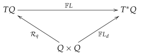
To appreciate this, we look at the interaction of three manifolds $Q\times Q$, $T^{\ast }Q$ and $TQ$. We take $(q_k,q_{k+1})$ to be the configuration variable q at successive time-step—it is the dynamical equation that governs the evolution from $q_k$ to $q_{k+1}$. The Hamiltonian dynamics, which is encoded in the preservation of ${\omega }_{can}$ of $T^{\ast }Q$, governs discrete Hamiltonian flow $H(q_k,p_k)$, through a Type I generating function $L_d(q_k,q_{k+1})$. On the other hand, the Lagrangian flow is governed by the retraction map ${\mathcal{R}}_q$, such as the Dirichlet-to-Neumann map induced by Jacobi’s solution $S_{q_0}\left(q\right)$ to the Hamilton–Jacobi equation. Those two dynamic updates $q_k\to q_{k+1}$ need not be identical. In mechanics, the Hamiltonian energy conservation system and the Lagrangian extremization system lead to one and the same dynamics, precisely because $L(q_k,v_k)$ and $H(q_k,p_k)$ are linked through the fiberwise Legendre transform $\mathbb{F}L$ at $q_k$:

$$L(q_k,v_k)+H(q_k,p_k)-{⟨v_k,p_k⟩}_{q_k}\equiv 0.$$

In other words, L and H are perfectly coupled–with no duality gap.

Information geometry, on the other hand, starts with a divergence (or contrast) function $\mathcal{D}(q,v,p)$ on $TQ\oplus T^{\ast }Q$, which measures the discrepancy between the two systems. Given $H(q,p)$ on $T^{\ast }Q$ and $L(q,v)$ on $TQ$, we write

$$\mathcal{D}(q,v,p)=L(q,v)+H(q,p)-{⟨v,p⟩}_q.$$

Theorem 2.

Let $L(q,v)$ and $H(q,p)$ be strictly convex functions, defined on $TQ$ and $T^{\ast }Q$ in terms of the variables $(q,v)$ and $(q,p)$, respectively. Then, for the following statements, any two imply the rest:

(i) 

$\mathcal{D}=0$;

(ii) 

$H(q,·)$ and $L(q,·)$ are (fiberwise) convex conjugate (Legendre dual) to each other;

(iii) 

$p=\frac{\partial L}{\partial v}=\mathbb{F}L\left(v\right)$ ;

(iv) 

$v=\frac{\partial H}{\partial p}=\mathbb{F}H\left(p\right)$ .

When $\mathcal{D}=0$, ${\omega }_L({\xi }_L,·)={\iota }_{{\xi }_L}{\omega }_L=d{E}_L$ with ${\xi }_L=(\dot{q},\dot{v})$, and

$$E_L(q,v)=\sum _i{v}^i\frac{\partial L(q,v)}{\partial v^i}-L(q,v).$$

Then,

$$d{E}_L=\sum _i\left(\sum _j\frac{{\partial }^{2}L}{\partial q^i\partial v^j}{v}^j-\frac{\partial L}{\partial q^i}\right)d{q}^i+\sum _{ij}{v}^j\frac{{\partial }^{2}L}{\partial v^i\partial v^j}d{v}^i.$$

The Euler–Lagrange equations are equivalent to

$${\xi }_L=\left(\frac{\partial E_L}{\partial q},\frac{\partial E_L}{\partial v}\right).$$

Our insight here is that $\mathcal{D}$ does not have to vanish identically. The consequence is that we do not require the Lagrangian dynamics (extremization dynamics) and Hamiltonian dynamics (conservation dynamics) to be coupled; they will be allowed to evolve independently. The function $\mathcal{D}$ allows us to study fiberwise symplectomorphisms of Dirac manifolds.

Let us consider the case that (ii) holds, i.e., $H(q,·)$ and $L(q,·)$ are Legendre duals to each other. Then, the canonical divergence $\mathcal{D}$ can be written as the Bregman divergence ${\mathcal{B}}_H$ and ${\mathcal{B}}_L$, after applying the fiberwise Legendre map $\mathbb{F}L$ or $\mathbb{F}H$,

$$p=\frac{\partial L(q,v)}{\partial v}⟺v=\frac{\partial H(q,p)}{\partial p}.$$

This implies that,

$$\begin{array}{cc}\hfill {\mathcal{B}}_L(q,v_0,v_1)& \equiv \mathcal{D}\left(q,v_0,\frac{\partial L(q,v)}{\partial v_1}\right)=L(q,v_1)-L(q,v_0)-⟨\frac{\partial L(q,v_0)}{\partial v_0},v_1-v_0⟩,\hfill \\ \hfill {\mathcal{B}}_H(q,p_0,p_1)& \equiv \mathcal{D}\left(q,\frac{\partial H(q,p_0)}{\partial p_0},p_1\right)=H(q,p_1)-H(q,p_0)-⟨\frac{\partial H(q,p_0)}{\partial p_0},p_1-p_0⟩,\hfill \end{array}$$

and they satisfy,

$${\mathcal{B}}_L(q,v_0,v_1)={\mathcal{B}}_H(q,p_1,p_0).$$

This is the reference-representation biduality [18,19], which is satisfied whenever L and H are Legendre duals of each other.

5.4. Variational Error Analysis

Recall that we previously defined the exact discrete Lagrangian $L_d^E$ (16), which is related to Jacobi’s solution of the Hamilton–Jacobi equation. The significance of the exact discrete Lagrangian is that it generates the exact discrete time flow of a Lagrangian system, but in general it cannot be computed explicitly. Instead, a computable discrete Lagrangian $L_d$ is used instead to construct a discretization of Lagrangian mechanics, and it induces the discrete Lagrangian map $F_{L_d}$.

Since discrete variational mechanics is expressed in terms of discrete Lagrangians, and the exact discrete Lagrangian generates the exact flow map of a continuous Lagrangian system, it is natural to ask whether we can characterize the order of accuracy of the Lagrangian map $F_{L_d}$ as an approximation of the exact flow map, in terms of the extent to which the discrete Lagrangian $L_d$ approximates the exact discrete Lagrangian $L_d^E$. This is indeed possible, and is referred to as variational error analysis. Theorem 2.3.1 of [11] shows that if a discrete Lagrangian $L_d$ approximates the exact discrete Lagrangian $L_d^E$ to order p, i.e., $L_d(q_0,q_1;h)=L_d^E(q_0,q_1;h)+\mathcal{O}\left(h^{p+1}\right)$, then the discrete Hamiltonian map, ${\tilde{F}}_{L_d}:(q_k,p_k)\mapsto (q_{k+1},p_{k+1})$, viewed as a one-step method, is order p accurate.

As mentioned above, the divergence function $\mathcal{D}$ from information geometry can serve as a Type I generating function of a symplectic map, and hence it can be viewed as a discrete Lagrangian in the sense of discrete Lagrangian mechanics. A divergence function also generates the Riemannian metric and affine connection structures on the diagonal manifold (Lemma 1), in addition to generating the symplectic structure on $Q\times Q$. Viewed in this way, a natural question is to what extent can we view the divergence function as corresponding to the exact Lagrangian flow of an associated continuous Lagrangian. We can show that

Theorem 3.

The exact discrete Lagrangian $L_d^E(q\left(0\right),q\left(h\right),h)$ associated with the geodesic flow, with respect to the induced metric g, can be approximated by a divergence function $\mathcal{D}\left(q\right(0),q(h\left)\right)$ up to third order $\mathcal{O}\left(h^3\right)$ accuracy,

$$L_d^E(q\left(0\right),q\left(h\right),h)=hL(q\left(0\right),v\left(0\right))+\mathcal{D}(q\left(0\right),q\left(h\right))+\mathcal{O}\left(h^3\right),$$

if and only if Q is a Hessian manifold, i.e., $\mathcal{D}$ is the Bregman divergence ${\mathcal{B}}_{\mathsf{\Phi }}$, for some strictly convex function Φ.

Proof. 

Let us expand the exact discrete Lagrangian to obtain,

$$\begin{array}{cc}\hfill L_d^E(q\left(0\right),q\left(h\right),h)& =hL(q,\dot{q})+\frac{h^2}{2}\left(\frac{\partial L}{\partial q}(q,\dot{q})+\frac{\partial L}{\partial \dot{q}}(q,\dot{q})·\ddot{q}\right)+\mathcal{O}\left(h^3\right)\hfill \\ & =hL(q,v)+\frac{h^2}{2}\left(\frac{\partial L}{\partial q^i}{v}^i+\frac{\partial L}{\partial v^i}{a}^i\right)+\mathcal{O}\left(h^3\right),\hfill \end{array}$$

(73)

where $q\left(0\right)=q,v=\dot{q}\left(0\right),a=\ddot{q}\left(0\right)$.

From the definition of a divergence function:

$${\mathcal{D}}_{,j}(q,q)=0.$$

Differentiating with respect to q,

$$0=\frac{\partial }{\partial q^i}{\mathcal{D}}_{,j}(q,q)={\mathcal{D}}_{i,j}(q,q)+{\mathcal{D}}_{,ij}(q,q),$$

so

$${\mathcal{D}}_{i,j}(q,q)=-{\mathcal{D}}_{,ij}(q,q).$$

Differentiating with respect to q again,

$$\frac{\partial }{\partial q^k}{\mathcal{D}}_{,ij}(q,q)={\mathcal{D}}_{k,ij}(q,q)+{\mathcal{D}}_{,ijk}(q,q).$$

Observe that the left-hand side is the metric induced by the divergence function,

$$\frac{\partial }{\partial q^k}{\mathcal{D}}_{,ij}(q,q)=-{\mathcal{D}}_{i,j}(q,q)=g_{ij}\left(q\right).$$

Expanding $\mathcal{D}(q,q^{\prime })$ around $q=q\left(0\right)$ for $q^{\prime }=q\left(h\right)$:

$$q^{\prime }=q+vh+\frac{1}{2}a{h}^2+\mathcal{O}\left(h^3\right),$$

we obtain

$$\mathcal{D}(q,q^{\prime })=\frac{h^2}{2}{g}_{ij}\left(q\right)+\frac{h^3}{4}{g}_{ij}\left(q\right)(v^i{a}^j+v^j{a}^i)+\frac{h^3}{6}{\Gamma }_{ijk}\left(q\right)v^i{v}^j{v}^k+\mathcal{O}\left(h^4\right),$$

where

$$\mathcal{D}(q,q)=0,{\mathcal{D}}_{,i}(q,q)=0,{\mathcal{D}}_{,ij}(q,q)\equiv g_{ij}\left(q\right)=-{\mathcal{D}}_{i,j}(q,q),{\mathcal{D}}_{,ijk}(q,q)\equiv {\Gamma }_{ijk}\left(q\right).$$

Clearly, $g_{ij}=g_{ji}$, and

$${\Gamma }_{ijk}={\Gamma }_{ikj}={\Gamma }_{kij}={\Gamma }_{kji}={\Gamma }_{jki}={\Gamma }_{jik}.$$

Comparing the corresponding terms in powers of h, we obtain,

$$\begin{array}{cc}\hfill L(q,v)& =\frac{1}{2}{g}_{ij}{v}^i{v}^j,\hfill \end{array}$$

(74)

$$\begin{array}{cc}\hfill v^i\frac{\partial L}{\partial q^i}(q,v)+a^i\frac{\partial L}{\partial v^i}(q,v)& =\frac{1}{2}{g}_{ij}(a^i{v}^j+a^j{v}^i)+\frac{1}{3}{\Gamma }_{ijk}{v}^i{v}^j{v}^k.\hfill \end{array}$$

(75)

Substituting (74) into (75) yields

$$\frac{\partial g_{ij}}{\partial q^k}={\Gamma }_{ijk},$$

with

$$\frac{\partial g_{ij}}{\partial q^k}=\frac{\partial g_{ik}}{\partial q^j}.$$

This, according to Proposition 1, demonstrates that the manifold $\mathbb{M}$ is Hessian, and hence dually-flat. So, for the expansions to agree to $\mathcal{O}\left(h^3\right)$, the inducing divergence function $\mathcal{D}$ must be the Bregman divergence ${\mathcal{B}}_{\mathsf{\Phi }}$. ☐

6. Summary

In this paper, we show the differences and connections between geometric mechanics and information geometry in canonically prescribing differential geometric structures on a smooth manifold Q. The Legendre transform plays crucial roles in both; however, they serve very different purposes. In geometric mechanics, the fiberwise Legendre map serves to link the cotangent bundle $T^{\ast }Q$ with tangent bundle $TQ$, whereas in information geometry, the Legendre transform relates the pair of biorthogonal coordinates, which are special coordinates on a dually-flat manifold Q. More specifically, $\mathbb{F}L$ (or its inverse $\mathbb{F}H$) is invoked to establish the isomorphism between $T^{\ast }Q\leftrightarrow TQ$ in geometric mechanics, whereas in information geometry, a Hessian metric g built upon a convex function on Q is used for the correspondence between two coordinate systems on Q, and also for potentially (but not necessarily) establishing a correspondence between $TQ$ and $T^{\ast }Q$.

The link between information geometry and discrete mechanics is much stronger when one considers the discrete version (as opposed to the traditional, continuous version) of geometric mechanics. Both endow a symplectic structure ${\omega }_{\times }$ on $Q\times Q$, through the use of a discrete Lagrangian $L_d$ in the case of geometric mechanics and a divergence function $\mathcal{D}$ in the case of information geometry—in fact they are both Type I generating functions for inducing ${\omega }_{\times }$ on $Q\times Q$ via pullback from the canonical symplectic structure ${\omega }_{can}$ on $T^{\ast }Q$. Using the Legendre transform, Type II generating functions can be constructed, which lead to the (right) discrete Hamiltonian $H^{+}$ in geometric mechanics and to the dual divergence function in information geometry.

Our analyses draw a distinction between the fiberwise Legendre map (which is used in continuous mechanics setting), the Legendre transform between biorthogonal coordinates (which is used in information geometry), and the Legendre transform between Type I and Type II generating functions (which is used in the setting of both discrete geometric mechanics and information geometry). The distinctions are more prominent when one considers the Pontryagin bundle $TQ\oplus T^{\ast }Q$. There, we can construct a divergence function that actually measures the duality gap between the Lagrangian function and the Hamiltonian function that generate a pair of (forward and backward) Legendre maps. In so doing, we demonstrate that information geometry can be viewed as an extension of geometric mechanics based on Dirac mechanics and geometry, with a full-blown duality between the Lagrangian and Hamiltonian components.

7. Discussion and Future Directions

Noda [24] showed that, with respect to the symplectic structure ${\omega }_{\times }$ on $Q\times Q$, the Hamiltonian flow of the canonical divergence $\mathcal{A}$ induces geodesic flows for ∇ and ${\nabla }^{\ast }$. He interpreted biorthogonal coordinates as a single coordinate system on $Q\times Q$, in a way that is consistent with treating $\mathcal{A}$ as the Type I generating function on $Q\times Q$. It remains unclear how the resulting Hamiltonian flow is related to dynamical flow on the Dirac manifold.

In another related work, Ay and Amari [25] sought to characterize the canonical form of divergence functions for general (non dually-flat) manifolds. They investigated the retraction map ${\mathcal{R}}_q:\left\{q\right\}\times Q\to T_{q}Q$ which we discussed in Section 2.5, and used the exponential map associated to any torsion-free affine connection ∇ on $TQ$. This approach, based on parallel transport, in essence generates a semispray on $TQ$, and is quite different from characterizing the dynamics using the Hamilton flow on $T^{\ast }Q$. Note that even though one may define a symplectic structure (through pullback) on $TQ$ as well, Ay and Amari [25] treats the semispray on $TQ$ as the primary geometric object. Future research will clarify its relation to our approach, which is based on defining a symplectic structure on $Q\times Q$ directly.

Finally, comparing information geometry with geometric mechanics may shed light on universal machine learning algorithms. In machine learning or state estimation applications, we wish to have the estimated distribution be influenced by the observations, so that the estimated distribution eventually becomes consistent with the observed data. Let $\left\{x_i\right\}$ denote the sequence of predictions by (possibly a series of) model distributions $\mathcal{X}$, and let $\left\{y_i\right\}$ denote the actual data generated by an unknown distribution $\mathcal{Y}$ that we are trying to estimate. In practice, the divergence functions are constructed so that the pseudo-distance between two distributions $\mathcal{X}$ and $\mathcal{Y}$ can be computed using only complete information about $\mathcal{X}$ and samples from $\mathcal{Y}$. As such, we can measure the mismatch between the current prediction $x_i$ and the actual data $y_i$ using $\mathcal{D}(x_i,y_i)$, since the asymmetry in the definition of $\mathcal{D}$ is such that we only require samples $y_i$ from the true but unknown distribution. So, adding a momentum term to ensure gentle change in model predictions, a possible choice of a discrete Lagrangian for generating the discrete dynamics for the machine learning application might be given by

$$L(x_i,x_{i+1})=\mathcal{D}(x_i,x_{i+1})+\mathcal{D}(x_{i+1},y_{i+1}),$$

where the first term can be interpreted as the action associated with the kinetic energy, and the second term is the action associated with the potential energy. By construction, the term $\mathcal{D}(x_i,y_i)$ vanishes when the prediction $x_i$ is consistent with the actual observation $y_i$, and it is positive otherwise, so the term $\mathcal{D}(x_i,y_i)$ can be viewed as a potential energy term that penalizes mismatch between the estimated distribution and the observational data. Our variational error analysis may thus shed light on an asymptotic theory of inference where sample size $N\to \infty$ is akin to discretization step $h\to 0$.

The link between geometric mechanics and information geometry, as revealed through our present investigation, is still rather preliminary. The possibility of a unified mathematical framework for information and mechanics is intriguing and remains a challenge for future research.