Abstract
Tests for dependence of continuous, discrete and mixed continuous-discrete variables are ubiquitous in science. The goal of this paper is to derive Bayesian alternatives to frequentist null hypothesis significance tests for dependence. In particular, we will present three Bayesian tests for dependence of binary, continuous and mixed variables. These tests are nonparametric and based on the Dirichlet Process, which allows us to use the same prior model for all of them. Therefore, the tests are “consistent” among each other, in the sense that the probabilities that variables are dependent computed with these tests are commensurable across the different types of variables being tested. By means of simulations with artificial data, we show the effectiveness of the new tests.
1. Introduction
Tests for dependence of continuous, discrete and mixed continuous-discrete variables are fundamental in science. The standard way to statistically assess if two (or more) variables are dependent is by using null-hypothesis significance tests (NHST), such as -test, Kendall’s τ, etc. However, these tests are affected by the drawbacks which characterize NHST [1,2,3]. An NHST computes the probability of getting the observed (or a larger) value of the statistics under the assumption that the null hypothesis of independence is true, which is obviously not the same as the probability of variables being dependent on each other, given the observed data. Another common problem is that the claimed statistical significance might have no practical impact. Indeed, the usage of NHST often relies on the wrong assumptions that p-values are a reasonable proxy to the probability of the null hypothesis and that statistical significance implies practical significance.
In this paper, we propose a collection of Bayesian dependence tests. The questions we are actually interested in—for example, Is variable Y dependent on Z? or Based on the experiments, how probable is Y dependent on Z?—are actually questions about posterior probabilities. Answers to these questions are naturally provided by Bayesian methods. The core of this paper is thus to derive Bayesian alternatives to frequentist NHST and to discuss their inference and results. In particular, we present three Bayesian tests for dependence of binary, continuous and mixed variables. All of these tests are nonparametric and based on the Dirichlet Process. This allows us to use the same prior model for all the tests we develop. Therefore, they are “consistent” in the sense that the probabilities of dependence we compute are commensurable across the tests. This is another main difference about such an approach and the use of p-values, since the latter usually cannot be compared across different types of tests.
To address the issue of how to choose the prior parameters in case of lack of information, we propose the use of the Imprecise Dirichlet Process (IDP) [4]. It consists of a family of Dirichlet processes with fixed prior strength and and prior probability measure free to span the set of all distributions. In this way, we obtain as a byproduct a measure of sensitivity of inferences to the choice of the prior parameters.
Nonparametric tests based on the Dirichlet Process and on similar ideas to those presented in this paper have also been proposed in [4] to develop a Bayesian rank test, in [5] for a Bayesian signed-rank test, in [6] for a Bayesian Friedman test and in [7] for a Bayesian test that accounts for censored data.
Several alternative Bayesian methods are available for testing of independence. The test of linear dependence between two continuous univariate random variables can be achieved by fitting a linear model and inspecting the posterior distribution of the correlation coefficient. A more sophisticated test based on a Dirichlet Process Mixture prior is instead presented in [8] to deal with linear and nonlinear dependences. Other methods were proposed for testing of independence based on a contingency table [9,10,11]. The main difference between these works and the work presented in this paper is that we provide tests for continuous, categorical (binary) and mixed variables using the same approach. This allows us to derive a very general framework to test independence/dependence (these tests could be used for instance for feature selection in machine learning [12,13,14,15]).
By means of simulations on artificial data, we use our test to decide if two variables are dependent. We show that our Bayesian test achieves equal or better results than the frequentist tests. We moreover show that the IDP test is more robust, in the sense that it acknowledges when the decision is prior-dependent. In other words, the IDP test suspends the judgment and becomes indeterminate when the decision becomes prior dependent. Since IDP has all the positive features of a Bayesian test and it is more reliable than the frequentist tests, we propose IDP as a new test for testing dependence.
2. Dirichlet Process
The Dirichlet Process was developed by Ferguson [16] as a probability distribution on the space of probability distributions. Let be a standard Borel space with Borel σ-field and be the space of probability measures on equipped with the weak topology and the corresponding Borel σ-field . Let be the class of all probability measures on . We call the elements nonparametric priors.
An element of is called a Dirichlet Process distribution with base measure α if for every finite measurable partition of , the vector has a Dirichlet distribution with parameters , where is a finite positive Borel measure on . Consider the partition and for some measurable set , then if from the definition of the DP we have that , which is a β distribution. From the moments of the β distribution, we can thus derive that:
where we have used the calligraphic letter to denote expectation with respect to the Dirichlet process. This shows that the normalized measure of the DP reflects the prior expectation of P, while the scaling parameter controls how much P is allowed to deviate from its mean . Let stand for the total mass of and stand for the probability measure obtained by normalizing . If , we shall also describe this by saying or, if , , where stands for the cumulative distribution function of .
Let and f be a real-valued bounded function defined on . Then the expectation with respect to the Dirichlet Process of is
One of the most remarkable properties of the DP priors is that the posterior distribution of P is again a DP. Let be an independent and identically distributed sample from P and , then the posterior distribution of P given the observations, denoted as , is
where is an atomic probability measure centered at and . This means that the Dirichlet Process satisfies a property of conjugacy, in the sense that the posterior for P is again a Dirichlet Process with updated unnormalized base measure . From Equations (1)–(3), we can easily derive the posterior mean and variance of and, respectively, posterior expectation of f. Hereafter we list some useful properties of the DP that will be used in the sequel (see Chapter 3 in [17]).
- (a)
- In case , since P is completely defined by its cumulative distribution function F, a-priori we say and a posteriori we can rewrite (3) as follows:where I is the indicator function and is the empirical cumulative distribution.
- (b)
- Consider an element which puts all its mass at the probability measure for some . This can also be modeled as for each .
- (c)
- Assume that , , and , , are independent, then Section 3.1.1. in [17]:
- (d)
- Let have distribution . We can writewhere , and . This follows from (b)–(c).
An issue in the use of the DP as prior measure on P is how to choose the infinite dimensional parameter in case of lack of prior information. There are two avenues that we can follow. The first assumes that prior ignorance can be modelled satisfactorily by a so-called noninformative prior. In the DP setting, the only noninformative prior that has been proposed so far is the limiting DP obtained for , which has been introduced by [16] and discussed by [18]. The second approach suggests that lack of prior information should be expressed in terms of a set of probability distributions. This approach known as Imprecise Probability [19,20,21] is connected to Bayesian robustness [22,23,24] and it has been extensively applied to model prior (near-)ignorance in parametric models. In this paper, we implement a prior (near-)ignorance model by considering a set of DPs obtained by fixing s to a strictly positive value and letting span the set of all distributions. This model has been introduced in [4] with the name of Imprecise Dirichlet Process (IDP).
3. Bayesian Independence Tests
Let us denote by X the vector of variables so that the n observations of X can be rewritten as
that is, a set of n vector-valued i.i.d. observations of X. We also consider an auxiliary variable together with X. We assume that are independent variables from the same unknown distribution and that , that is, we have the same observations of X and .
Let P be the unknown distribution of and assume that the prior distribution of P is . Our goal is to compute the posterior of P. The posterior of P is given in (3) and, by exploiting (6), we know that
with and . The distribution of is similarly defined.
The questions we pose in a statistical analysis can all be answered by querying this posterior distribution in different ways. We adopt this posterior distribution to devise Bayesian counterparts of the independence hypothesis tests.
3.1. Bayesian Bivariate Independence Test for Binary Variables
Let us assume that the variables (that is, they are binary). Our aim is to devise a Bayesian independence test for binary variables based on the DP. We will also show that our test is a Bayesian generalisation of the frequentist -test for independence applied to binary variables. We start by defining the following quantities:
where we have exploited the independence of and here denotes the posterior cumulative distribution of defined in (8). From (8), it can easily be verified that
where
and
where in the last equality we have exploited the fact that has the same distribution as X and also the same observations. The two quantities include two terms. The first is the term due to the prior and the second term is due to the observations.
Similarly, we compute
where
and
Summing up, represent the posterior probabilities of the events (that is, and ), , and , respectively, according to the posterior joint distribution .
Theorem 1.
The variables Y and Z are said to be concordant (dependent) with posterior probability provided that
and they are said to be discordant provided that
where is the probability computed with respect to and . Finally, they are said to be simply dependent with posterior probability provided that
where denotes the posterior Highest Density Interval of .
Proof.
We just derive the third statement. The other two statements are analogue. We first consider the indicator functions
and same for the auxiliary variables . By computing the expectation of these functions, we can obtain the marginals of the variables with respect to the joint :
where (resp. ) denotes the marginal with respect to Z when (resp. ), while (resp. ) denotes the marginal with respect to Y when (resp. ).
Then, by exploiting independence between X and , we derive
We are now ready to define the independence test. If the two variables are independent, then the vector
has zero mean. Note that the first component of the vector v is and thus is a well-defined quantity with respect to our probabilistic model (similarly for the other terms). Therefore, the independence test reduces to checking whether the highest density credible region (HCR) of v includes the zero vector. It can be easily verified that for each component of v. In fact, we have
for and , , and so
Therefore, it is enough to check whether
If this is the case, then we can declare that the two variables are dependent with probability . Here, the multiplier 2 in is only a scaling factor so that varies in . ☐
From the proof of Theorem 1 it is evident the similarity of the test with the frequentist -test for independence. Both tests use the difference between the joint and the product of the marginals as a measure of dependence. The advantage of the Bayesian approach is that we compute posterior probabilities for the hypothesis in which we are interested and not the probability of getting the observed (or a larger) difference under the assumption that the null hypothesis of independence is true.
The probabilities computed in Theorem 1 depend on the prior information . In this paper we adopt IDP as prior model. We can then perform a Bayesian nonparametric test that is based on extremely weak prior assumptions, and easy to elicit, since it requires only the choice of the strength s of the DP instead of its infinite-dimensional parameter . The infinite-dimensional parameter is free to vary in the set of all distributions.
Let us consider for instance (13). Each one of these priors gives a posterior probability . We can characterize this set of posteriors by computing the lower and upper bounds and . Inferences with IDP can be computed by verifying if
and then by taking the following decisions:
- if both the inequalities are satisfied, then we declare that the two variables are dependent with probability larger than ;
- if only one of the inequalities is satisfied (which has necessarily to be the one for the upper), we are in an indeterminate situation, that is, we cannot decide;
- if both are not satisfied, then we declare that the probability that the two variables are dependent is lower than the desired probability of .
When IDP returns an indeterminate decision, it means that the evidence from the observations is not enough to declare that the probability of the hypothesis being true is either larger or smaller than the desired value ; more observations are necessary to reach a reliable decision.
Theorem 2.
The upper probability is obtained by a prior measure with
where and . The lower probability is obtained by a prior measure with the same m as before but and .
Proof.
We are interested in the quantity . It is clear that in order to maximize the probability that we must put all the prior mass on . Let us call . Then . From (9)–(12), we have that and with . By computing the derivative with respect to m we have
whose zero is , which is also a maximum. Hence, the maximum can be either on or on the extremes or . This can be easily verified by checking when (so ) or (so ). The lower probability can be determined using a similar reasoning. ☐
Since , the computation of , can be obtained by Monte Carlo sampling. The following pseudo-code describes how to compute the upper (the lower can be computed in a similar way).
- Initialize the counter to 0 and the array V to empty;
- For
- (a)
- sample ;
- (b)
- compute as in (9)–(12) by choosing with m defined in Theorem 2;
- (c)
- compute and store the result in V;
- (d)
- if then else .
- compute the histogram of the elements in V (this gives us the plot of the posterior of )
- compute the posterior upper probability that is greater than zero as .
The number of Monte Carlo samples is equal to 100 thousand in the next examples and figures.
The lower and upper intervals in Theorem 1 can also be obtained as in Theorem 2 and computed via Monte Carlo sampling ( can be computed using the values stored in V, see pseudo-code). Hereafter we will denote the two intervals corresponding to the lower and upper distributions as and , respectively.
The only prior parameter that must be selected with IDP is the prior strength s. The value of s determines how quickly the posteriors corresponding to the lower and upper probabilities converge as the number of observations increases. We select —this means that we need at least 4 concordant binary observations to take a decision with . In other words, for we need two observations of type and two of type to guarantee that both intervals, i.e., and , do not include the zero. For any number of (and configuration of) observations less than four, the test is always indeterminate (i.e., no decision can be taken). Thus, four is the minimum number of observations that is required to take a decision. This choice is arbitrary and subjective, but is our measure of cautiousness. We make clearer the meaning of determinate and indeterminate in the following example.
Example 1.

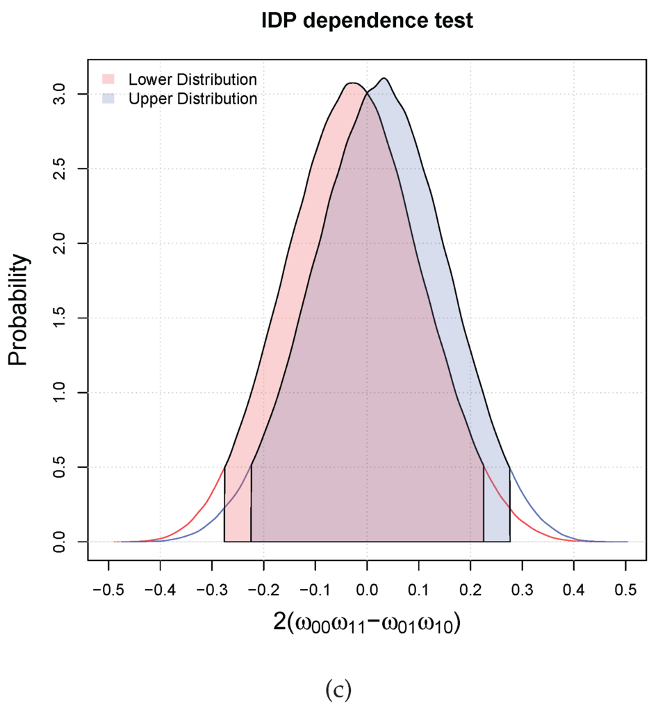
Let us consider the following three matrices of 10 paired binary i.i.d. observations
They correspond to different degrees of dependence. Figure 1 shows the lower and upper distributions of and the relative HDI, i.e., and , for the three cases (the filled in areas). In case (a), the two variables are dependent (concordant) with probability greater than , since all the mass of the lower and upper distributions are in the interval . In the second case, we are in an indeterminate situation, that is, the lower and upper are in disagreement, which means that the inference is prior dependent. In the third case, we can only say that they are not dependent at since both the intervals include the zero.


Figure 1.
Three possible results of the independence hypothesis testing with two binary variables. The red and blue filled areas correspond respectively to the lower and upper . (a) Dependent at ; (b) Indeterminate at ; (c) They are not dependent at .
3.2. Bayesian Bivariate Independence Test for Continuous Variables
Let us assume that variables , that is, they are real continuous variables. Our aim is to devise a Bayesian independence test for continuous variables based on the DP. We will also show that our test is a Bayesian generalisation of Kendall-τ test for independence. This test uses results from [25] that derived a Bayesian Kendall’s τ statistic using DP. As before, we introduce auxiliary variables . We start by defining the following quantities:
and are concordance measures. We can then compute
where we have exploited the independence of and here denotes the posterior cumulative distribution of . This quantity is equal to
where we have exploited the fact that has the same distribution as X and the same observations. Given , it can be seen that the first two terms depend on the prior distribution and the last term is only due to the observations.
Theorem 3.
The variables Y and Z are said to be concordant (dependent) with posterior probability provided that
and they are said to be discordant provided that
where is the probability computed with respect to and . Finally, they are said to be simply dependent with posterior probability provided that
where denotes the posterior Highest Density Interval of .
The divisor 2 in is only a scaling factor so that the expectation lies in . The theorem simply follows from the fact that is the same measure of dependence used in Kendall’s τ test. In this respect, it is worth to highlight the connection with Kendall’s τ. By exploiting the properties of DP, we have that the posterior mean of for large n is approximately equal to.
and this is exactly Kendall’s sample τ coefficient. In fact, Kendall’s sample τ coefficient is defined as:
with
Observe that T can also be rewritten as:
in terms of all the pairs, which is proportional to (30) for large n. This clarifies the connection between our Bayesian test of dependence for continuous variables based on and Kendall’s τ test.
As for the dependence test for binary variables, we will make inferences using IDP. Inferences with IDP can computed by verifying if
Theorem 4.
The upper probability is obtained by a prior measure with for . The lower probability is obtained by a prior measure with and and for .
Proof.
We have that
We want to maximize . Since , we need at least two Dirac’s deltas. Hence, we consider the mixture with for . Then we have that
and so we have maximized the second term. For the first term depending on , the maximum is obtained at . For the lower probability, the proof is similar. ☐
The lower and upper intervals can also be obtained as in Theorem 4. Again in this case, the value of s determines how quickly lower and upper posteriors converge as the number of observations increases. We choose as for the binary test.
Example 2.

Also in this case we consider three matrices of 10 paired continuous i.i.d. observations
They correspond to different degrees of dependence. Figure 2 shows the lower and upper posteriors for the three cases and the relative intervals at probability (the filled in areas). In case (a), the two variables are dependent (concordant) with probability greater than , since all the mass of the lower and upper distributions are in the interval . In the second case, we are in an indeterminate situation, that is, the lower and upper are in disagreement, which means that the inference is prior dependent. In the third case, we can only say that they are not dependent at since both the intervals include the zero.

Figure 2.
Three possible results of the independence hypothesis testing for continuous variables. The red and blue filled areas correspond respectively to the lower and upper . (a) Dependent at ; (b) Indeterminate at ; (c) They are not dependent at .
3.3. Bayesian Bivariate Independence Test for Mixed Continuous-Binary Variables
Let us assume that the variables and . Our aim is to devise a Bayesian independence test based on the DP. We introduce the auxiliary variable as done before. To derive our test, we start by defining the following indicator:
This indicator is one if and , with and zero otherwise. We can compute
where we have exploited the independence of . denotes the posterior cumulative distribution of . This quantity is equal to
For large n, we have that
which is equal to the rank of Y in the observations with respect to the observations . Therefore, our dependence test is rank-based. It is clear that, in the case of independence of the variables Y and Z, the mean rank is equal to . Hence, we can formulate an independence test for mixed variables.
Theorem 5.
The variables Y and Z are dependent with posterior probability provided that
where denotes the posterior Highest Density Interval of .
The theorem follows from the fact that in case of independence between variables Y and Z the mean rank (36) scaled by 4 and shifted of is equal to 0. Also in this case, we make inferences using IDP.
Theorem 6.
The upper probability is obtained by a prior measure with equal to and equal to and
with and . The lower probability is obtained by a prior measure with equal to .
Proof.
Consider the quantity
and with equal to and equal to . Thus
By computing the derivative
we have that . The result is obtained by exploiting the fact that . For the lower probability, the computation is straightforward. ☐
The lower and upper intervals can also be obtained as in Theorem 4. We choose as for the previous tests.
Example 3.
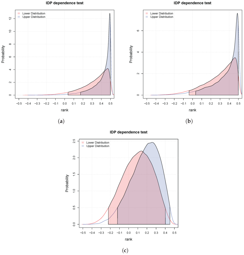
We consider three matrices of 10 paired binary-continuous i.i.d. observations
Again, they correspond to different degrees of dependence. Figure 3 shows the lower and upper posteriors for the three cases and the relative intervals at probability (the filled in areas). In case (a), the two variables are dependent (concordant) with probability greater than , since all the mass of the lower and upper distributions are in the interval . In the second case, we are in an indeterminate situation, that is, the lower and upper are in disagreement. In the third case, we can only say that they are not dependent at since both the intervals include the zero.

Figure 3.
Three possible results of the independence hypothesis testing for pairs binary-continuous. The red and blue filled areas correspond respectively to the lower and upper . (a) Dependent at ; (b) Indeterminate at ; (c) They are not dependent at .
4. Experiments
We compare our Bayesian testing approach in the three discussed main scenarios where both variables are binary, both are continuous and one is binary and the other is continuous. The goal is to decide whether the two variables are dependent or independent. We generate n samples ( and 50) using the distributions defined in Table 1. Ten thousand repetitions are used by forcing the variables to be independent (so ) and thousand repetitions where the variables are dependent, for each value of . The value of β is varied as explained in the table. For each n, β and each of these twenty thousand samples (for which we know the correct result of the test), we run the new approach versus test, Kendall τ test and Kolmogorov–Smirnov test, respectively for the binary-binary, continuous-continuous and binary-continuous cases. For each run of each method, we record their p-values, while for the new approach we compute γ corresponding to the limiting credible region wide where the decision changes between dependent and independent. Such value is related to the p-values of the other tests and can be used for decision making by comparing it against a threshold (just as it is done with the p-values). However, it should be observed that thresholds different from or are hardly used in practice in null hypothesis significance tests. Conversely, for a Bayesian tests is a probability and, therefore, we can take decisions with probability , but also or even depending on the application (and the loss function). However, instead of fixing a threshold (which is a subjective choice) to decide between the options dependent and non-dependent with probability , we use Receiver Operating Characteristic (ROC) curves. ROC curves give the quality of the approaches for all possible thresholds. The curves are calculated as usual by varying the threshold from 0 to 1 and computing the sensitivity (or true positive rate) and specificity (or one minus false positive rate) (this is slightly different from the common approach of drawing ROC curves as a function of the true positive rate and false positive rate [26,27,28]). ROC curves are always computed considering different degrees of dependence (different values for ) against independence (). We apply the same criterion to p-values for comparing the methods across a wider range of decision criteria. We have used the R package “pROC” to compute the ROC curves [29].

Table 1.
Data generation setup. In order to generate independent data, β is set to zero. Larger values of β increase their dependency.
Figure 4, Figure 5 and Figure 6 present the comparison of the new approach (which we name as IBinary, ICont or IMixed to explicitly account for the types of variables been analyzed) using against the appropriate competitor. With such choice of s, the new approach runs without indeterminacy and can be directly compared against usual methods. As we see in the figures, the new method performs very similar to each competitor, with the advantage of being compatible among different types of data (the p-values of the other methods, among different data types, cannot be compared to each other). This is useful when one works with multivariate models involving multiple data types. As expected, the quality of the methods increases with the increase of β and of the sample size.

Figure 4.
Comparison of approaches with binary data. New approach with (so always determinate) is compared against test using ROC curves. Curves are built using two thousand repetitions (one thousand where variables are independent () and one thousand where they are dependent with β as shown in the figures). Data are generated as explained in Table 1. (a) ROC (, ); (b) ROC (, ); (c) ROC (, ); (d) ROC (, ).
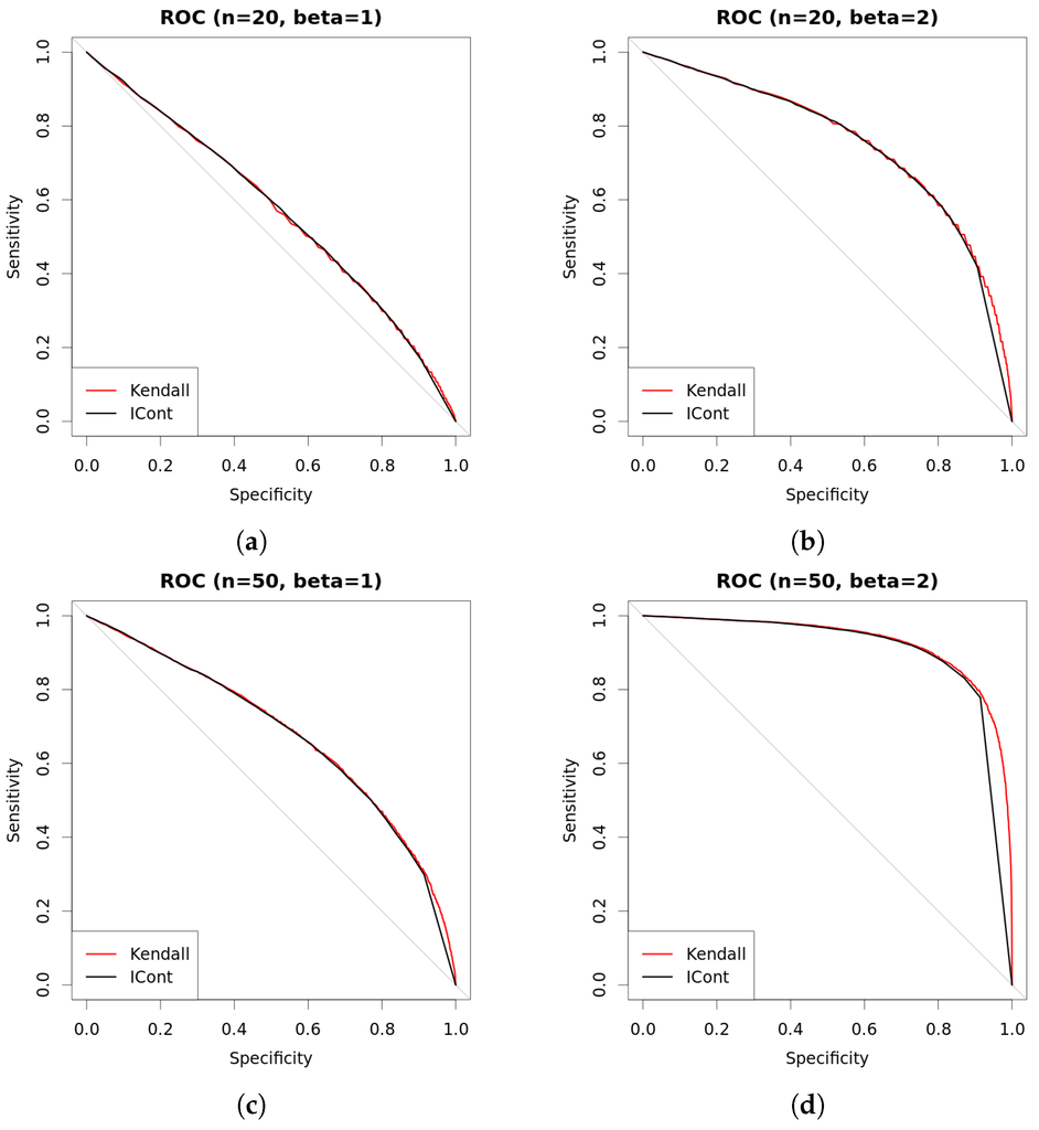
Figure 5.
Comparison of approaches with continuous data. New approach with (so always determinate) is compared against Kendall test using ROC curves. Curves are built using two thousand repetitions (one thousand where variables are independent () and one thousand where they are dependent with β as shown in the figures). Data are generated as explained in Table 1. (a) ROC (, ); (b) ROC (, ); (c) ROC (, ); (d) ROC (, ).
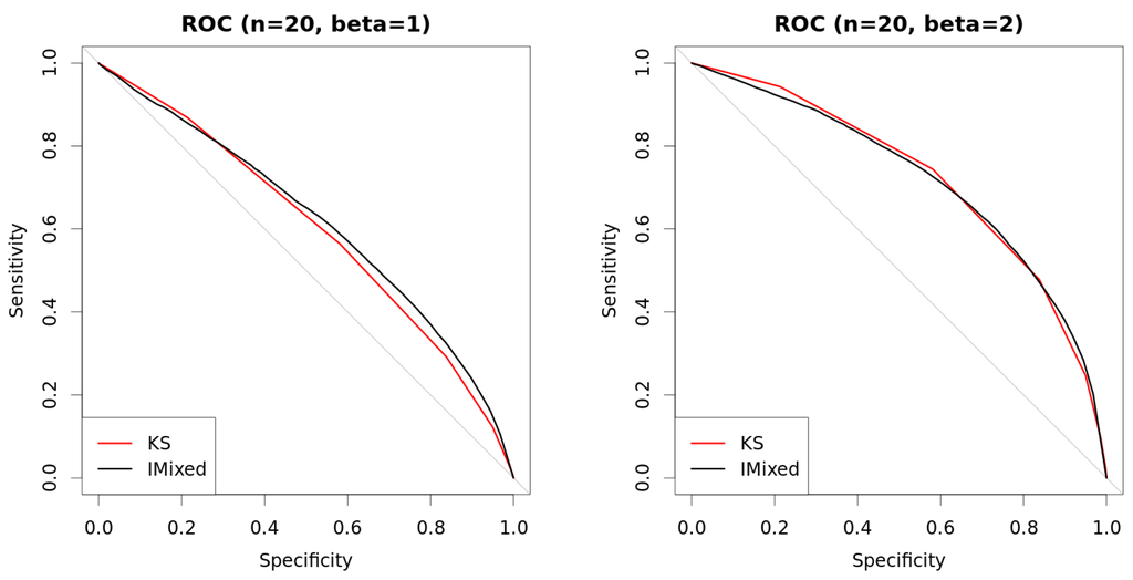
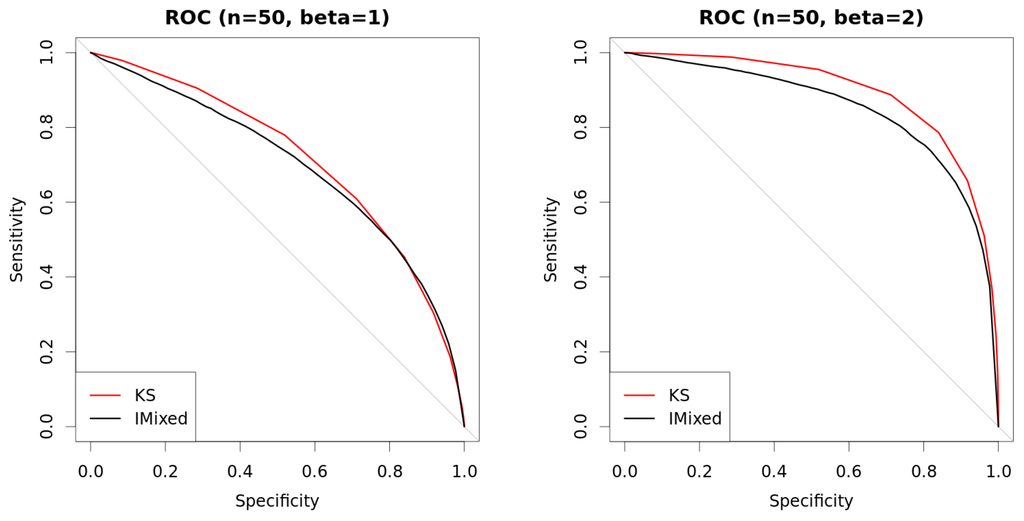
Figure 6.
Comparison of approaches with mixed data. New method with (so always determinate) is compared against Kolmogorov–Smirnov (KS) test using ROC curves. Curves are built using two thousand repetitions (one thousand where variables are independent () and one thousand where they are dependent with β as shown in the figures). Data are generated as explained in Table 1. (a) ROC (, ); (b) ROC (, ); (c) ROC (, ); (d) ROC (, ).
Figure 7, Figure 8 and Figure 9 present the ROC curves for the methods , Kendall τ and Kolmogorov–Smirnov, respectively. These curves are separated according to whether the instance is considered determinate or indeterminate by the new approach. In other words, for each one of the twenty thousand repetitions, we run the corresponding usual test and then we check whether the output of the new approach is determinate or indeterminate (applying ), and we split the instances accordingly (blue curves show the accuracy over instances that are considered easy (determinate cases) while green curves over instances that are hard (indeterminate cases)—we also present the overall accuracy of the method using red curves). As we see, such division is able to identify easy-to-classify and hard-to-classify cases, since the ROC curves for the cases deemed as indeterminate by the new approach suggest a performance not better than a random guess (green curves). using the new approach, This means that if we would devise another test (called “50/50 when indeterminate”) which returns the same response as IBinary, ICont or IMixed when they are determinate, and issues a random answer (with 50/50 chance) otherwise, then this “50/50 when indeterminate” test would have the same ROC curve as , Kendall τ and Kolmogorov–Smirnov, respectively.

Figure 7.
Comparison of approaches with binary data. New approach is used to differentiate instance by instance into hard-to-classify and easy-to-classify, and curves represent the outcome of test under each such different scenarios. Data are generated as explained in Table 1. (a) ROC (, ); (b) ROC (, ); (c) ROC (, ); (d) ROC (, ).
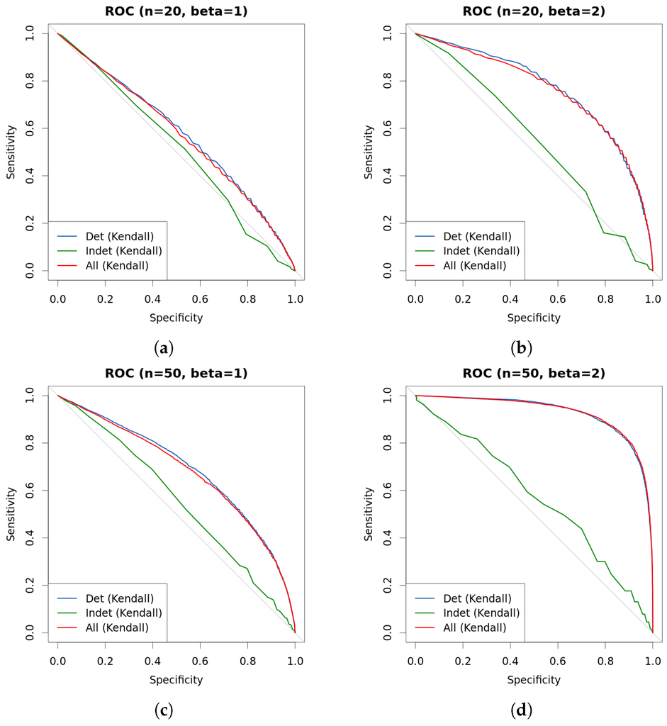
Figure 8.
Comparison of approaches with continuous data. New approach is used to differentiate instance by instance into hard-to-classify and easy-to-classify, and curves represent the outcome of Kendall τ test under each such different scenarios. Data are generated as explained in Table 1. (a) ROC (, ); (b) ROC (, ); (c) ROC (, ); (d) ROC (, ).
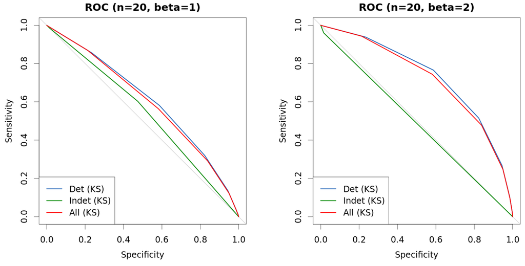
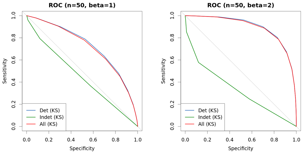
Figure 9.
Comparison of approaches with mixed data. New approach is used to differentiate instance by instance into hard-to-classify and easy-to-classify, and curves represent the outcome of Kolmogorov–Smirnov (KS) test under each such different scenarios. Data are generated as explained in Table 1. (a) ROC (, ); (b) ROC (, ); (c) ROC (, ); (d) ROC (, ).
This suggests that the indeterminacy of IDP based tests is an additional useful information that our approach gives to the analyst. In these cases she/he knows that (i) her/his posterior decisions would depend on the choice of the prior DP measure; (ii) deciding between the two hypotheses under test is a difficult problem as shown by the comparison with the DP with , , Kendall τ and Kolmogorov–Smirnov. Based on this additional information, the analyst can for example decide to collect additional measurements to eliminate the indeterminacy (in fact when the number of observations goes to infinity the indeterminacy goes to zero).
This represents a second advantage of our IDP approach, once we have fixed the value of s (e.g., ) it can automatically identify the risky cases where a decision must be taken with additional caution. For this reason, we suggest to use the IDP based test for dependence and not .
Finally, Table 2, Table 3 and Table 4 present the values for the Area under the curve (AUC) in Chaper 5 in [30] of the ROC curves discussed previously, as well as similar experimental setup but with different values of s: 0.25, 0.5 and 1. Table 2 has results for binary variable versus binary variable, Table 3 for continuous variable versus continuous variable, and Table 4 for continuous variable versus binary variable. Overall, results show that IBinary has similar performance as test, ICont has similar performance as Kendall’s τ test and IMixed is similar to Kolmogorov–Smirnov (KS) test. The most interesting outcome is the comparison, in each scenario, of the frequentist test over whole data, over only data samples that were considered determinate by the new test, and over only data samples that were considered indeterminate. We clearly see that the AUC values over the cases considered indeterminate are much inferior to the values over cases considered determinate, which indicates that the new test has a good ability to discriminate easy and hard cases. ROC curves for values of s other than 0.5 were omitted for clarity of exposition, but they are very similar to those obtained for .

Table 2.
Area under the ROC curve (AUC) values for all the performed experiments using different values of s, β and n. IBinary shows the AUC for the new test applied to two binary variables and . The columns test, Det.cases, and Indet.cases show the AUC obtained by the test over all samples, only over samples considered determinate by IBinary (with the corresponding s) and finally only over samples considered indeterminate by IBinary.

Table 3.
Area under the ROC curve (AUC) values for all the performed experiments using different values of s, β and n. ICont shows the AUC for the new test applied to two continuous variables and . Kendall, Det.cases, and Indet.cases show the AUC obtained by Kendall’s test over all samples, only over samples considered determinate by ICont (with the corresponding s) and finally only over samples considered indeterminate by ICont.

Table 4.
Area under the ROC curve (AUC) values for all the performed experiments using different values of s, β and n. IMixed shows the AUC for the new test applied to one binary and one continuous variables and . Kolmogorov–Smirnov (KS), Det.cases, and Indet.cases show the AUC obtained by KS test over all samples, only over samples considered determinate by IMixed (with the corresponding s) and finally only over samples considered indeterminate by IMixed.
5. Conclusions
We have proposed three novel Bayesian methods for performing independence tests for binary, continuous and mixed binary-continuous variables. All of these tests are nonparametric and based on the Dirichlet Process. This has allowed us to use the same prior model for all the tests we have developed. Therefore, all the tests are “consistent”, in the sense that the probabilities of dependence we compute with these tests are commensurable across the tests.
We have presented two versions of these tests: one based on a noninformative prior and one based on a conservative model of prior ignorance (IDP). Experimental results show that the prior ignorance method is more reliable than both the frequentist test and the noninformative Bayesian one, being able to isolate instances in which these tests are almost guessing at random. For future work, we plan to extend this approach in two directions: (1) feature selection in classification; (2) learning the structure (graph) of Bayesian networks and Markov Random Fields. The idea is to use our dependence tests to replace the frequentist tests that are commonly used for that purpose and evaluate the gain in terms of performance. For instance in case (1), we then could compare the accuracy of a classifier whose features are selected using our tests with that of a classifier whose features are selected by using frequentist tests. Our new approach is suitable since it addresses two limitations of currently used tests: they are based on null-hypothesis significance tests, and they cannot be applied to categorical and continuous variables at the same time in a commensurable way.
Author Contributions
All authors made substantial contributions to conception and design, data analysis and interpretation of data; all authors participate in drafting the article or revising it critically for important intellectual content; all authors gave final approval of the version to be submitted.
Conflicts of Interest
The authors declare no conflict of interest.
Abbreviations
The following abbreviations are used in this manuscript:
| DP | Dirichlet Process |
| IDP | Imprecise Dirichlet Process |
References
- Raftery, A.E. Bayesian model selection in social research. Sociol. Methodol. 1995, 25, 111–164. [Google Scholar] [CrossRef]
- Goodman, S.N. Toward evidence-based medical statistics. 1: The P–value fallacy. Ann. Intern. Med. 1999, 130, 995–1004. [Google Scholar] [CrossRef] [PubMed]
- Kruschke, J.K. Bayesian data analysis. Wiley Interdiscip. Rev. Cognit. Sci. 2010, 1, 658–676. [Google Scholar] [CrossRef] [PubMed]
- Benavoli, A.; Mangili, F.; Ruggeri, F.; Zaffalon, M. Imprecise Dirichlet Process With Application to the Hypothesis Test on the Probability that X ≤ Y. J. Stat. Theory Pract. 2015, 9, 658–684. [Google Scholar] [CrossRef]
- Benavoli, A.; Mangili, F.; Corani, G.; Zaffalon, M.; Ruggeri, F. A Bayesian Wilcoxon Signed-Rank Test Based on the Dirichlet Process. In Proceedings of the 31st International Conference on Machine Learning (ICML), Beijing, China, 21–26 July 2014; pp. 1026–1034.
- Benavoli, A.; Corani, G.; Mangili, F.; Zaffalon, M. A Bayesian Nonparametric Procedure for Comparing Algorithms. In Proceedings of the 32nd International Conference on Machine Learning (ICML), Lille, France, 6–11 July 2015; pp. 1–9.
- Mangili, F.; Benavoli, A.; de Campos, C.P.; Zaffalon, M. Reliable survival analysis based on the Dirichlet Process. Biom. J. 2015, 57, 1002–1019. [Google Scholar] [CrossRef] [PubMed]
- Kao, Y.; Reich, B.J.; Bondell, H.D. A nonparametric Bayesian test of dependence. 2015; arXiv:1501.07198. [Google Scholar]
- Nandram, B.; Choi, J.W. Bayesian analysis of a two-way categorical table incorporating intraclass correlation. J. Stat. Comput. Simul. 2006, 76, 233–249. [Google Scholar] [CrossRef]
- Nandram, B.; Choi, J.W. Alternative tests of independence in two-way categorical tables. J. Data Sci. 2007, 5, 217–237. [Google Scholar]
- Nandram, B.; Bhatta, D.; Sedransk, J.; Bhadra, D. A Bayesian test of independence in a two-way contingency table using surrogate sampling. J. Stat. Plan. Inference 2013, 143, 1392–1408. [Google Scholar] [CrossRef]
- Friedman, N.; Geiger, D.; Goldszmidt, M. Bayesian network classifiers. Mach. Learn. 1997, 29, 131–163. [Google Scholar] [CrossRef]
- Blum, A.L.; Langley, P. Selection of relevant features and examples in machine learning. Artif. Intell. 1997, 97, 245–271. [Google Scholar] [CrossRef]
- Keogh, E.J.; Pazzani, M.J. Learning Augmented Bayesian Classifiers: A Comparison of Distribution-Based and Classification-Based Approaches. Available online: http://www.cs.rutgers.edu/∼pazzani/Publications/EamonnAIStats.pdf (accessed on 31 August 2016).
- Jiang, L.; Cai, Z.; Wang, D.; Zhang, H. Improving Tree augmented Naive Bayes for class probability estimation. Knowl. Based Syst. 2012, 26, 239–245. [Google Scholar] [CrossRef]
- Ferguson, T.S. A Bayesian Analysis of Some Nonparametric Problems. Ann. Stat. 1973, 1, 209–230. [Google Scholar] [CrossRef]
- Ghosh, J.K.; Ramamoorthi, R. Bayesian Nonparametrics; Springer: Berlin/Heidelberg, Germany, 2003. [Google Scholar]
- Rubin, D.B. Bayesian Bootstrap. Ann. Stat. 1981, 9, 130–134. [Google Scholar] [CrossRef]
- Walley, P. Statistical Reasoning with Imprecise Probabilities; Chapman & Hall: New York, NY, USA, 1991. [Google Scholar]
- Coolen-Schrijner, P.; Coolen, F.P.; Troffaes, M.C.; Augustin, T. Imprecision in Statistical Theory and Practice. J. Stat. Theory Pract. 2009, 3. [Google Scholar] [CrossRef]
- Augustin, T.; Coolen, F.P.; de Cooman, G.; Troffaes, M.C. Introduction to Imprecise Probabilities; John Wiley & Sons: Hoboken, NJ, USA, 2014. [Google Scholar]
- Berger, J.O.; Rios Insua, D.; Ruggeri, F. Bayesian Robustness. In Robust Bayesian Analysis; Insua, D.R., Ruggeri, F., Eds.; Springer: Berlin/Heidelberg, Germany, 2000; Volume 152, pp. 1–32. [Google Scholar]
- Berger, J.O.; Moreno, E.; Pericchi, L.R.; Bayarri, M.J.; Bernardo, J.M.; Cano, J.A.; De la Horra, J.; Martín, J.; Ríos-Insúa, D.; Betrò, B.; et al. An overview of robust Bayesian analysis. Test 1994, 3, 5–124. [Google Scholar] [CrossRef]
- Pericchi, L.R.; Walley, P. Robust Bayesian credible intervals and prior ignorance. Int. Stat. Rev. 1991, 59. [Google Scholar] [CrossRef]
- Dalal, S.; Phadia, E. Nonparametric Bayes inference for concordance in bivariate distributions. Commun. Stat. Theory Methods 1983, 12, 947–963. [Google Scholar] [CrossRef]
- Tan, P.-N.; Steinbach, M.; Kumar, V. Introduction to Data Mining; Pearson Education: New York, NY, USA, 2006. [Google Scholar]
- Jiang, L.; Li, C.; Cai, Z. Learning decision tree for ranking. Knowl. Inf. Syst. 2009, 20, 123–135. [Google Scholar] [CrossRef]
- Jiang, L.; Wang, D.; Zhang, H.; Cai, Z.; Huang, B. Using instance cloning to improve naive Bayes for ranking. Int. J. Pattern Recognit. Artif. Intell. 2008, 22, 1121–1140. [Google Scholar] [CrossRef]
- Robin, X.; Turck, N.; Hainard, A.; Tiberti, N.; Lisacek, F.; Sanchez, J.C.; Müller, M. pROC: An open-source package for R and S+ to analyze and compare ROC curves. BMC Bioinform. 2011, 12. [Google Scholar] [CrossRef] [PubMed]
- Murphy, K.P. Machine Learning: A Probabilistic Perspective; MIT Press: Cambridge, MA, USA, 2012. [Google Scholar]
© 2016 by the authors; licensee MDPI, Basel, Switzerland. This article is an open access article distributed under the terms and conditions of the Creative Commons Attribution (CC-BY) license (http://creativecommons.org/licenses/by/4.0/).