1. Introduction
Analysis of real-world graphs can be greatly simplified by using artificial generative graph models, which we will refer to as theoretical graph models throughout this paper. These models try to mimic the mechanisms responsible for the emergence of graph phenomena by means of a simple generative procedure. The main advantage of theoretical graph models is that they provide analytic solutions to several graph problems. Over the years, numerous theoretical graph models have been proposed in the scientific literature. Most of these models focus on producing graphs which exhibit certain properties, such as a particular distribution of vertex degrees, edge betweenness, or local clustering coefficients. Sometimes a model might be proposed to explain an unexpected empirical result, such as shrinking graph diameter or the densification of edges. Each such theoretical graph model is governed by a small set of parameters, but many models are unstable, i.e., they produce significantly different graphs in response to even a minuscule modification of parameter values.
When faced with an empirical graph, researchers often want to approximate the graph by a theoretical graph model, for instance to derive analytically bounds on certain graph properties, or simply to be able to compare the empirical graph with similar other graphs originating from the same family. However, as we have previously mentioned, the choice of the proper theoretical graph model is not trivial since the shape and properties of artificially generated graphs depend so strongly on the values of the main parameter of the model. In addition, the inherent randomness of theoretical graph models produces individual realizations which can differ significantly within a single model and a single parameter setting. Thus, the similarity of the empirical graph to a single realization of a theoretical graph model can be purely incidental.
In this work we test the usefulness of traditional centrality measures in comparing graphs, and verify if additional features, namely, the entropy of centrality measure distributions, may allow for better graph comparisons. We analyze the behavior of theoretical graph models under changing model parameters and observe the stability of centrality measures. The results of our experiments clearly suggest that enriching graph properties with entropy of centrality measures allows for much more accurate comparisons of graphs. In addition we show how accurate is the comparison of graphs using Kolmogorov–Smirnov (K-S) test of distances between distributions when applied to distributions of degree, betweenness, local clustering coefficient, and vertex entropy. The results tend to suggest that the K-S test is of little help when trying to assign a graph to one of the theoretical graph models.
This paper is organized as follows. In
Section 2 we review previous applications of entropy in graphs.
Section 3 contains basic definitions, centrality measures, and a brief description of theoretical graph models used in our experiments. Then we propose the method for graph comparison and classification in
Section 4. We describe our experiments and discuss the results in
Section 5. The paper concludes in
Section 6 with a brief summary and future work agenda.
2. Related Work
Although the notion of entropy is quite well-established in computer science [
1] and has even a long application history in graphs analytics [
2], there is no agreed upon definition of entropy in the world of graphs. For instance, Allegrini et al. approach the entropy as the fundamental measure of complexity of every complex system, and they show that if entropy is to be perceived as the measure of complexity, this leads to several conflicting definitions of entropy. The entropies discussed by Allegrini et al. can be divided into three main groups. Thermodynamic-based entropies of Clausius and Boltzmann assume that all components of a complex system can be treated as statistically independent and that they all follow identical and independent distributions, with no interference or interactions with other components. Statistical entropies, such as Gibbs entropy [
3] or entropy proposed by Tsallis et al. [
4] generalize thermodynamic-based entropies by allowing individual components of a complex system to be described by unequal probabilities. This allows to combine activity of individual components at the microscale with the overall behavior of the complex system. A special case of statistical entropies are entropies developed in the field of information theory, most notably Shannon entropy [
5], Kolmogorov–Sinai entropy [
6], and Renyi entropy [
7]. These entropies measure the amount of information present in a system and can be used to describe the transmission of messages across the system. In these approaches it is assumed that the entropy, as a measure of uncertainty, is a non-decreasing function of the amount of available information.
Apart from trying to adapt classical definitions of entropy to graphs, many researchers tried to propose new formulas specifically tailored to the structure of graphs. For instance, Li et al. [
8] define the topological entropy by measuring the number of all possible configurations that can be produced by the process generating the graph for a given set of parameters. The more ”deterministic” the process is, i.e., the smaller the uncertainty about the final configuration of the graph, the smaller the entropy of the graph. Sole and Valverde redefine the classical Shannon entropy using the distribution of vertex degrees in the graph [
9]. In [
10,
11], the authors propose to derive interrelations of graph distance measures by means of inequalities in topological indices combined with distance measures derived from Wiener index, Randić index and eigenvalue-based quantities. Another approach has been proposed by Körner [
12] who defined graph entropy based on the notion of stable sets of a graph (a set of vertices is stable if no two vertices from the set are adjacent), but unfortunately the problem of finding stable sets is NP-hard, which significantly limits the usability of Körner entropy in large graphs. Recently, Dehmer proposed to define graph entropy based on information functionals [
13] which are monotonic functions defined on sets of associated objects of a graph (sets of vertices, sets of edges, subgraphs). This approach nicely generalizes several previous, more specific proposals. Information functionals allow to define many kinds of related network entropies based on degrees and distances. For instance, Cao et al. [
14] use the notion of information functionals to define degree-based graph entropy and establish limits on extremal values of such graph entropy for certain families of graphs. The information functional introduced in [
15] and defined as the number of vertices with distance
k to a given vertex establishes the distance-based graph entropy. Finally, it is worth noting that recent works have tackled the problem of graph entropy for weighted graphs, albeit in a limited way [
16,
17].
Graph entropy has been studied extensively in the field of network coding. Riis introduces the private entropy of a directed graph and relates it to the guessing number of the graph [
18]. This work is further expanded by Gadouleau and Riis [
19] by proposing the notion of the guessing graph and finding specific directed graphs with high guessing number which are capable of transferring large amounts of information. The relationship between perfect graphs and graph entropy is examined in detail by Simonyi [
20]. Perfect graphs are a very important class of graphs, in which many problems, such as graph coloring, maximum clique problem, or maximum independent vertex set problem can be solved in polynomial time.
In [
21,
22] authors summarize the methods for performing a comparative graph analysis and explain the history, foundations and differences of such techniques. It is underlined that distinguishing between methods for deterministic and random graphs is important for a better understanding of the interdisciplinary setting of data science to solve a particular problem involving comparative network analysis.
3. Basic Definitions
Given a graph
, where
is the set of vertices, and
is the set of edges, where each edge is an unordered pair of vertices from the set
V. Given a function
which associates a numerical weight with every edge. In this work we consider only undirected graphs, thus each edge is represented as a set of two vertices rather than an ordered pair of vertices. In order to characterize the graph
G we introduce the following centrality measures [
23].
3.1. Centrality Measures
3.1.1. Degree
The degree of the vertex
v is the number of edges incident to
v:
Degree is a natural measure of vertex importance. Vertices with high degrees tend to play central roles in many graphs and are considered by many to be the focal points of graph functionality.
3.1.2. Betweenness
Let
be a sequence of vertices such that any two consecutive vertices in the sequence form an edge in the graph
G. Such a sequence is referred to as a
path between vertices
and
. The shortest path is defined as
The intuition behind the betweenness centrality measure is that if there are many shortest paths traversing vertex
v, this vertex is important from the point of view of communication and flow through the graph. Formally, the betweenness of a vertex is defined as:
where
denotes a shortest path between vertices
and
traversing through the vertex
v. Betweenness is often considered to be a good measure of vertex importance with respect to information transmission, and vertices with the highest betweenness tend to be communication hubs which facilitate communication in the graph.
3.1.3. Local Clustering Coefficient
Given the vertex
v, we may consider the
ego network of
v which consists of the vertex
v, its direct neighbours, and all edges between them,
, where
and
. An interesting characteristic of a single vertex is the connection pattern in its ego network. This can be expressed as the
local clustering coefficient defined as:
where
. Simply put, the local clustering coefficient of a vertex
v is the ratio of the number of edges in the ego network of
v to the maximum number of edges that could exist in this ego network (i.e., if the ego network of
v formed a clique). The local clustering coefficient reaches its minimum when the ego network of the vertex
v has a star formation and its value informs how well connected the direct neighbours of
v are.
3.1.4. Vertex Entropy
The last centrality measure computed by us for all theoretical graph models is the vertex entropy, also known as
diversity. The vertex entropy of the vertex
v is simply the scaled Shannon entropy of the weighs of all edges adjacent to
v. Formally, vertex entropy is defined as:
Vertex entropy measures for each vertex the unexpectedness of edge weights for all edges adjacent to a given vertex. This measure can also be very easily modified to measure the inequality of edge weights.
All these centrality measures are commonly used to describe macro-properties of various graphs. In particular, distributions of degrees, betweennesses, and local clustering coefficients are often perceived as sufficient characterizations of a graph. In the remaining part of the paper we will try to show why this approach is wrong and leads to erroneous conclusions.
3.2. Graph Models
Over the years several theoretical graph models have been proposed. Most of these models try to construct a method of generating graphs that would display certain properties which are frequent in empirical graphs. For instance, the prevalence of real-world social networks displays the power-law distribution of vertex degrees [
24]. Many dynamic graphs show surprising behavior when examined along the time dimension, like the shrinking diameter of the graph as the number of vertices grow, or the slow densification of edges in relation to the number of vertices [
25]. Theoretical graph models presented in the literature try to capture these behaviors using simple rules of edge creation and deletion. In this section we briefly overview the most popular theoretical graph models used in our experiments.
3.2.1. Random Graph
The random graph model, also known as the Erdős–Rényi model, has been first introduced by Paul Erdős and Alfréd Rényi in [
26]. There are two versions of the model. The
model consists in randomly selecting a single graph
g from the universe of all possible graphs having
n vertices and
M edges. The second model, dubbed
, creates the graph
g by first creating
n isolated vertices, and then creating, for each pair of vertices
, an edge with the probability
p. Due to much easier implementation and analytical accessibility, the
model is far more popular and this is the model we have used in our experiments. Properties of the graph generated according to the
model depend strongly on the
ratio. If this ratio exceeds 1 (which means that the average degree of the random vertex approaches 1), we observe the phenomenon of percolation in which almost all isolated components quickly merge to form a single giant component. During this merging phase the betweenness distribution changes drastically.
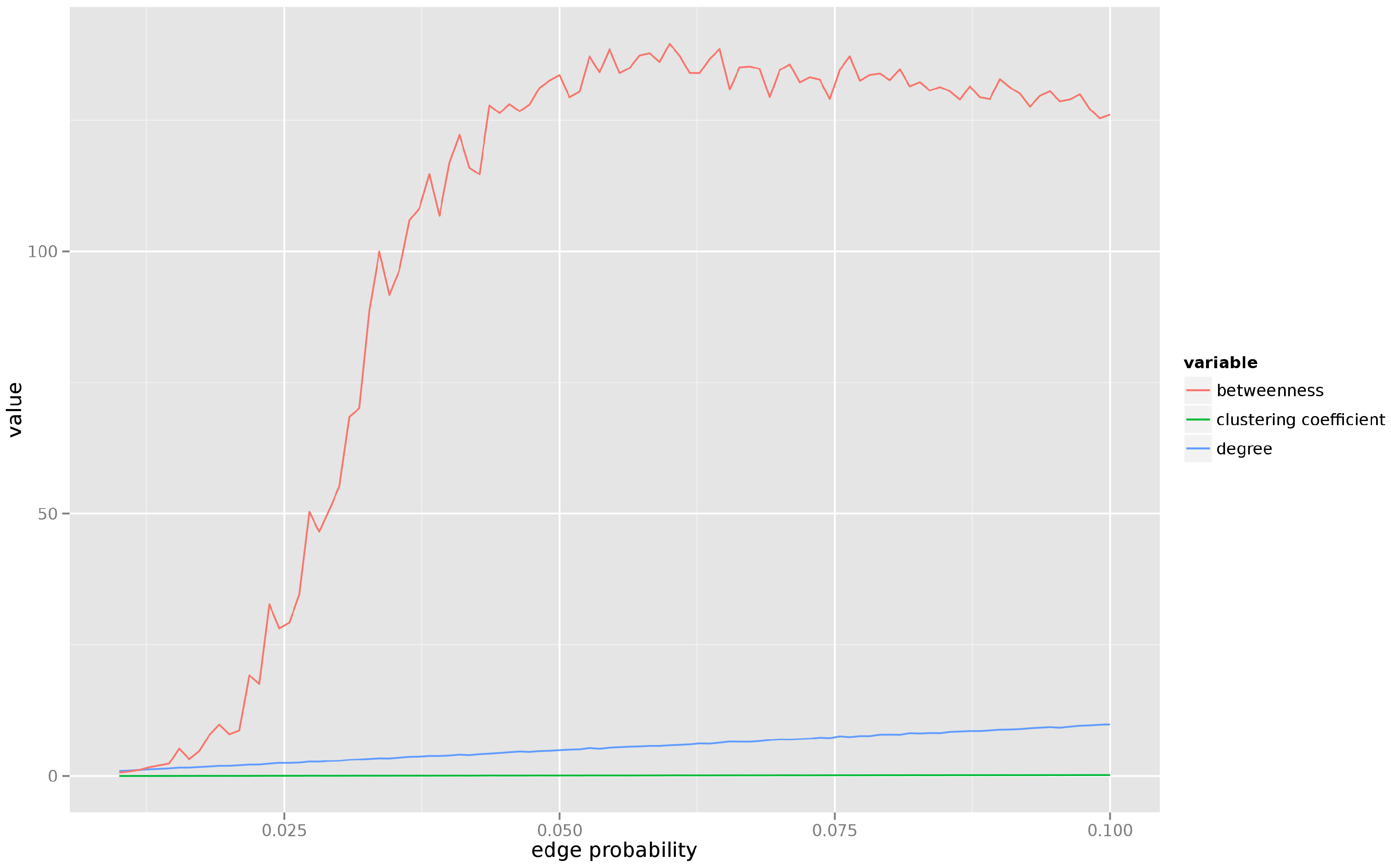
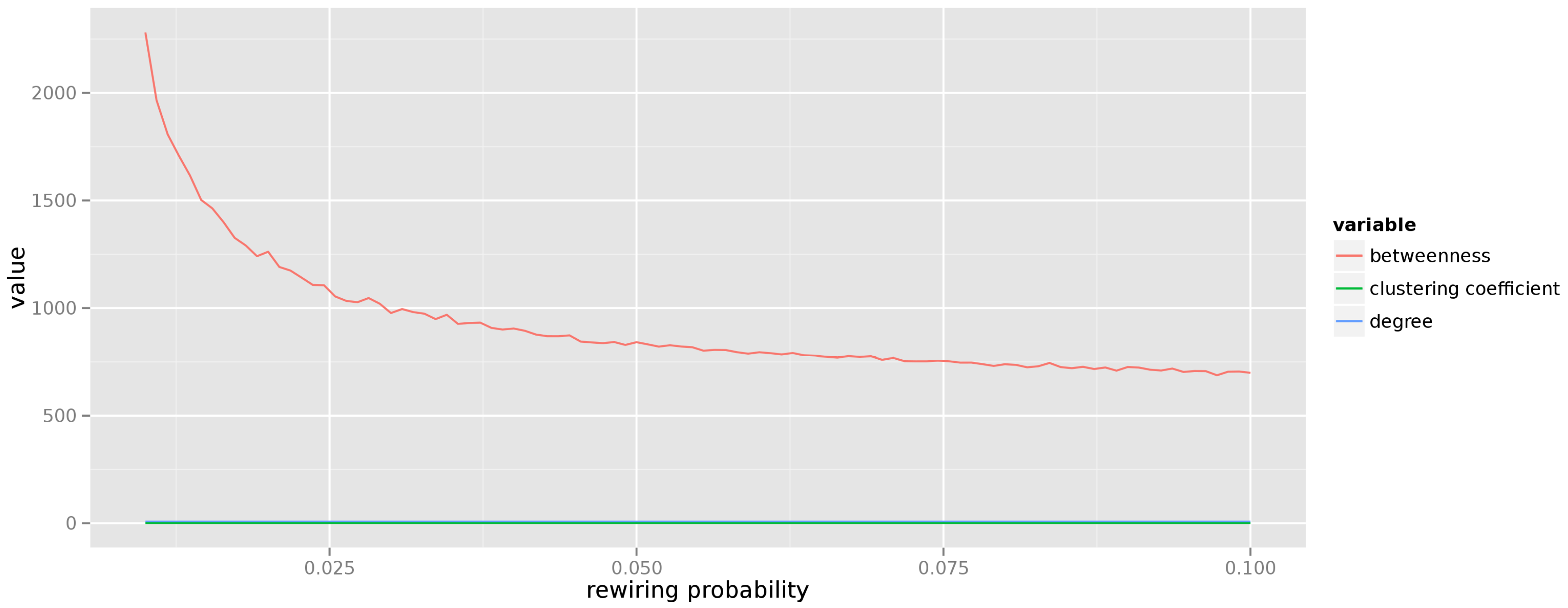
Figure 1 presents average degree, betweenness, and clustering coefficient for a graph consisting of
vertices and the probability of edge creation changing from
to
. Each value on the graph is an average of 50 independently generated graphs for a given
combination. We can see that the clustering coefficient remains constant, the average degree grows very slowly, but the betweenness undergoes a rapid transformation and, after the percolation, settles at a much higher level in the denser graph.
3.2.2. Small World
The small world model has been introduced by Duncan Watts and Steven Strogatz in [
27]. According to this model, a set of
n vertices is organized into a regular circular lattice, with each vertex connecting directly with
k of its nearest neighbours. After creating the initial lattice, each edge is rewired with the probability
p, i.e., an edge
is replaced with the edge
where
is selected uniformly from
V.
The resulting graphs have many interesting features.
Figure 2 presents the aggregated measures for graphs created from
vertices with the neighbour size of 4 and the edge rewire probability varying from
to
(again, each point is the average of 50 realizations of the graph for a given combination of
parameters). It is easy to see that the graphs generated according to the small world model display constant degree and local clustering coefficients (indeed, random rewiring of just a few edges does not impact these values), whereas the average betweenness tends to drop (more vertices begin acting as communication hubs as more edges become rewired). In addition, the average path length in a small world graph is short and falls rapidly with the increase of the edge rewire probability
p. When
the small world graph becomes the random graph.
3.2.3. Preferential Attachment
There is a whole family of graph models collectively referred to as “preferential attachment” models. Basically, any model in which the probability of forming an edge to a vertex is proportional to that vertex degree can be classified as a preferential attachment model. The first attempt to use the mechanism of preferential attachment to generate artificial graphs can be attributed to Derek de Solla Price who tried to explain the process of formation of scientific citations by the advantageous cumulation of citations by prominent papers [
28].
Another well-known model which utilizes the same mechanism has been proposed by Albert–László Barabási and Réka Albert [
29]. According to this model, the initial graph is a full graph
with
vertices. All subsequent vertices are added to the graph one by one, and each new vertex creates
m edges. The probability of choosing the vertex
as the endpoint of a newly created edge is proportional to current degree of
and can be expressed as
. The resulting graph displays the power law distribution of vertex degrees because of the quick accumulation of new edges by prominent vertices. Interestingly, the model encompasses two processes simultaneously: the graph continues to grow and new vertices are constantly added, at the same time the preferential attachment process creates hubs. The authors of the model limited each of these processes independently, resulting in graphs with either geometric or Gaussian degree distributions. Thus, graph growth or preferential attachment alone do not produce scale-free structures of power law graphs.
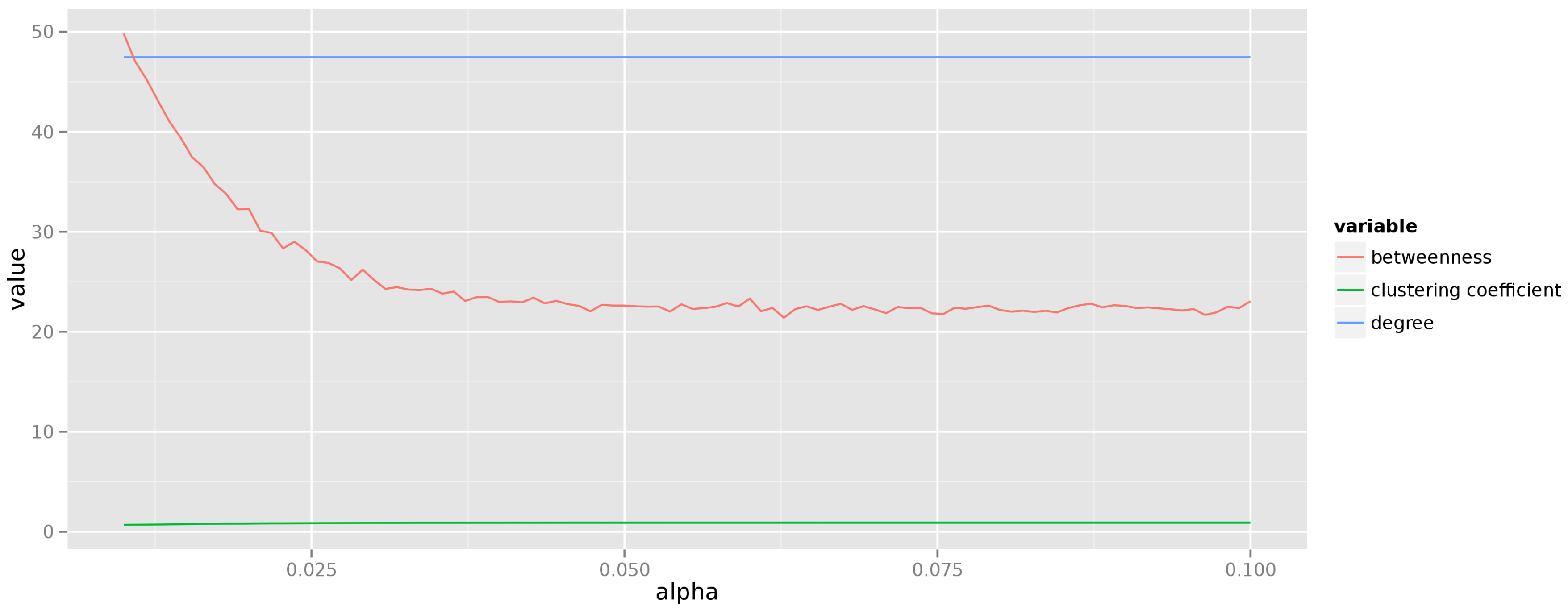
Figure 3 shows the average degree, betweenness, and clustering coefficient for graphs consisting of
vertices generated according to the Barabási–Albert model (each measurement is averaged over 50 instances of the graph generated for a given exponent
α, where the probability of creating an edge to a vertex
v with degree
is given as
). These results are quite misleading though, because for an individual instance the distribution of both degree and betweenness follows the power law, thus the very notion of an “average” is questionable.
3.2.4. Forest Fire
This model has been introduced by Jure Leskovec et al. [
30] and tried to explain two phenomena commonly observed in real-world social networks. Firstly, contrary to popular belief, the diameter of most networks tends to shrink as more and more vertices are added. Secondly, most networks become denser over time, i.e., the number of edges in the network grows super-linearly in the number of vertices. The forest fire model works as follows. Vertices are added sequentially to the graph. Upon arrival each vertex creates an initial edge to
n vertices called
ambassadors, which are selected uniformly from the set of existing vertices. Next, with the
forward burning probability p the newly added vertex begins to ”burn” neighbours of each ambassador, creating edges to ”burned” vertices. The fire spreads recursively, i.e., the burning of neighbouring vertices is repeated for every vertex to which an edge has been created. This model, according to its authors, tries to mimic the mechanism of real forest fire, but it can be also easily translated into the way people find new acquaintances. Graphs generated using the forest fire model exhibit not only the densification of edges and the shrinking diameter of the graph, but also preserve the power-law distributions of in-degrees and out-degrees.
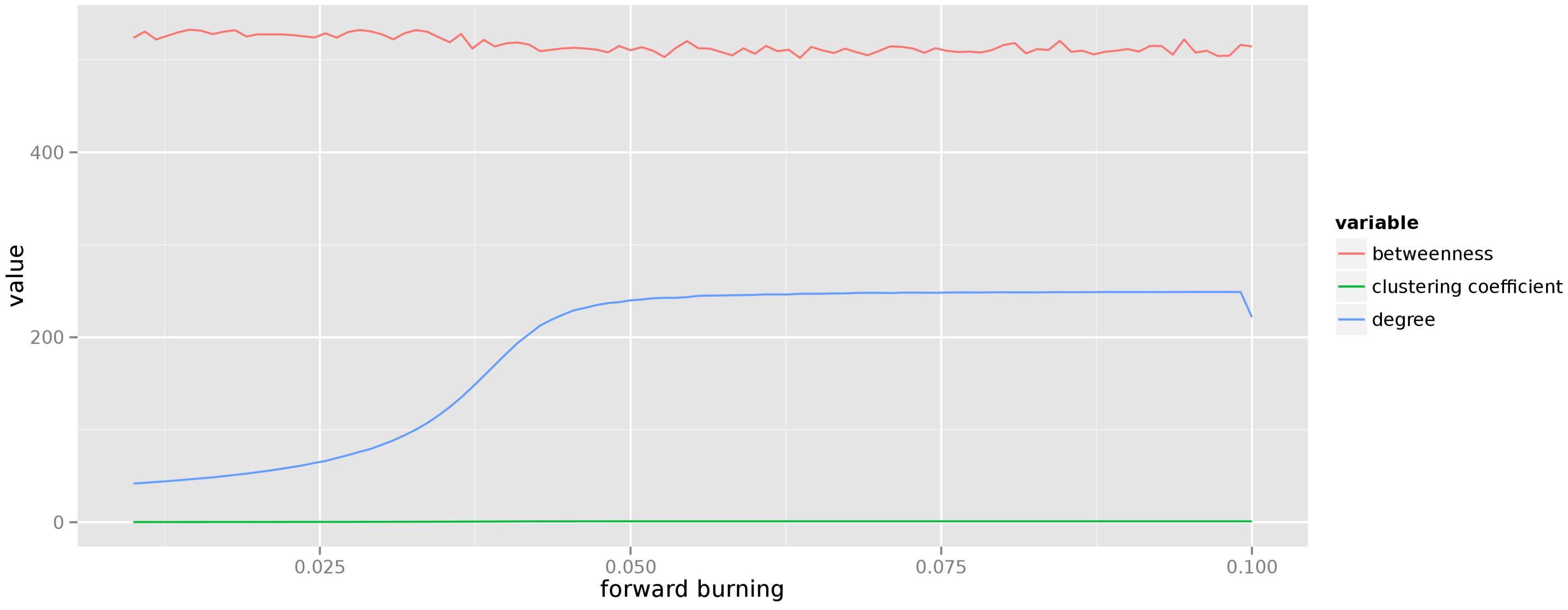
The change of centrality measures for graphs generated from the forest fire model is presented in
Figure 4. The forward burning probability varies from
to
and for each value of this parameter 50 graphs are generated, each consisting of 250 vertices. As can be seen, the forest fire model generates graphs in which vertices have high betweenness and very low local clustering coefficient (the dominating structures in the graph are star-shaped). The average degree changes in a sigmoid fashion and asymptotically reaches a stable value.
4. The Method for Graph Comparison and Classification
Our proposed method for graph comparison and classification is based on a simple unsupervised learning approach and uses a distance metric between a particular empirical graph and the graphs generated by theoretical graph models in order to classify the empirical graph to the theoretical graph model. The main idea is to classify graphs by comparing structural feature distributions of vertices. In order to make distributions suitable for unsupervised learning (which usually requires a metric space), we propose an aggregation function of the distributions. When applied to distributions of structural measures of vertices, denoted by , e.g., degree, betweenness, local clustering coefficient, the aggregation produces a single point in space which represents a given graph. Representing graphs in such space allows calculating the distance between graphs. Thus, any particular empirical graph could be compared to and classified as an example of a theoretical graph model.
In order to provide the classification for empirical graphs the proposed unsupervised learning approach is based on a non-parametric method called k-nearest neighbours. It is similar to kernel methods with a random and variable bandwidth. The idea is to base estimation of the class on the fixed number of k graphs representations which are the closest to the graph under evaluation, given some distance metric.
Let us suppose that graphs are represented in the space
and a sample
is available. For any fixed point
corresponding to a theoretical graph model we can calculate the distance to each
, e.g. by using Euclidean distance
, see Equation (
1).
The order of the distances composes a ranking or “nearest neighbors” list, i.e., and ranks sample graphs by how close they are to x. Then, based on majority voting from classes of k nearest graphs, the particular is labeled with the appropriate class. The procedure is depicted in Algorithm 1.
| Algorithm 1 The method for graph comparison and classification. |
- Input:
empirical graph , set of model graphs , empty space , set of aggregation functions , set of structural measures - 1:
for each graph x do - 2:
/* initialization of the vector representation of distributions in the space S */ - 3:
for each structural measure do - 4:
/* structural measure distributions for graphs */ - 5:
end for - 6:
/* calculate aggregation of structural measure distributions */ - 7:
end for - 8:
for each pair , do - 9:
calculate distances - 10:
end for - 11:
perform majority voting from distances for - 12:
return
|
5. Experiments, Results and Discussion
We have performed three different experiments aiming at the evaluation of the usefulness of graph entropy in graph classification:
The first experiment examines the stability of the mean entropy of centrality measure distributions under varying parameters of the theoretical graph models.
The second experiment assesses the improvement of classification accuracy of graphs when using centrality measure entropies as features.
The third experiment explores the power of the K-S test to correctly classify graphs.
In the following sections we describe the experiments in detail and we discuss obtained results.
5.1. Stability of Entropy
For each theoretical graph model we have created 5000 instances of graphs. We have chosen 100 different values of the main parameter of a given theoretical graph model, and for each value of the main parameter we have generated 50 instances of graphs. We have conducted our experiments on graphs having 50, 250, and 1000 vertices. For the sake of clarity we will report the results for graphs with 50 vertices. All results presented in this section are averaged over these 50 realizations of a particular graph model with the main parameter set. For each resulting graph realization we have computed the distribution of four centrality measures: degree, betweenness, local clustering coefficient, and vertex entropy. Then, we have computed the traditional Shannon entropy of each distribution. The results are presented below.
5.1.1. Random Graph Model
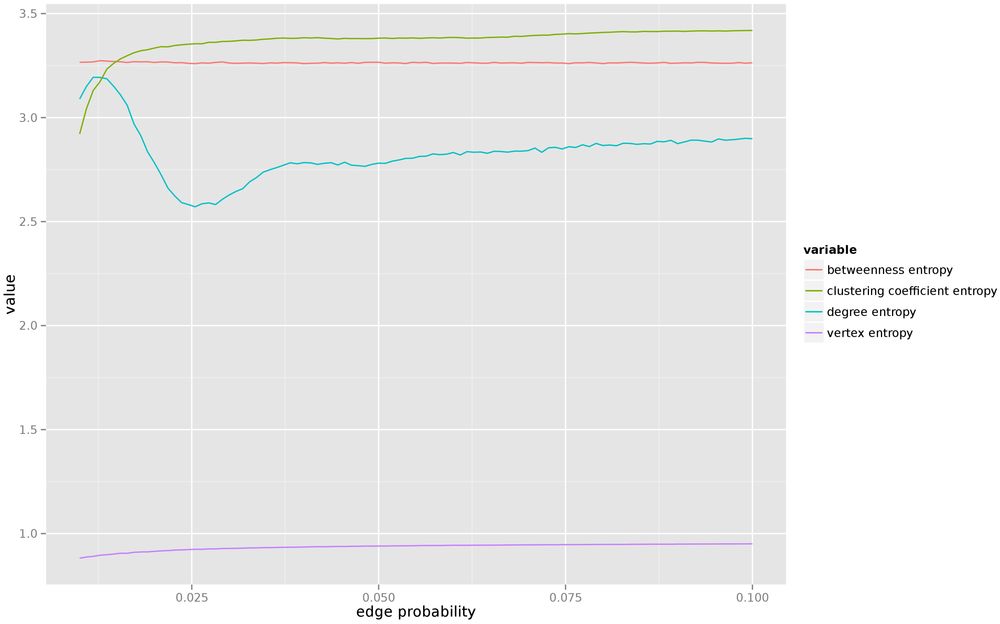
For this model we have varied the probability of edge creation from
to
.
Figure 5 presents the results. As one can see, for very low values of edge creation probability (when the resulting graph consists of several connected components) the entropy of most centrality measures is unstable, but as soon as the average degree of each vertex reaches 1, the entropy of all centrality measures quickly stabilizes. We also observe that there is little uncertainty about the vertex entropy, but the entropy of the remaining centrality measures remains relatively high (which agrees with the intuition, in a random graph the properties of each individual vertex can vary significantly from vertex to vertex.
5.1.2. Small World Model
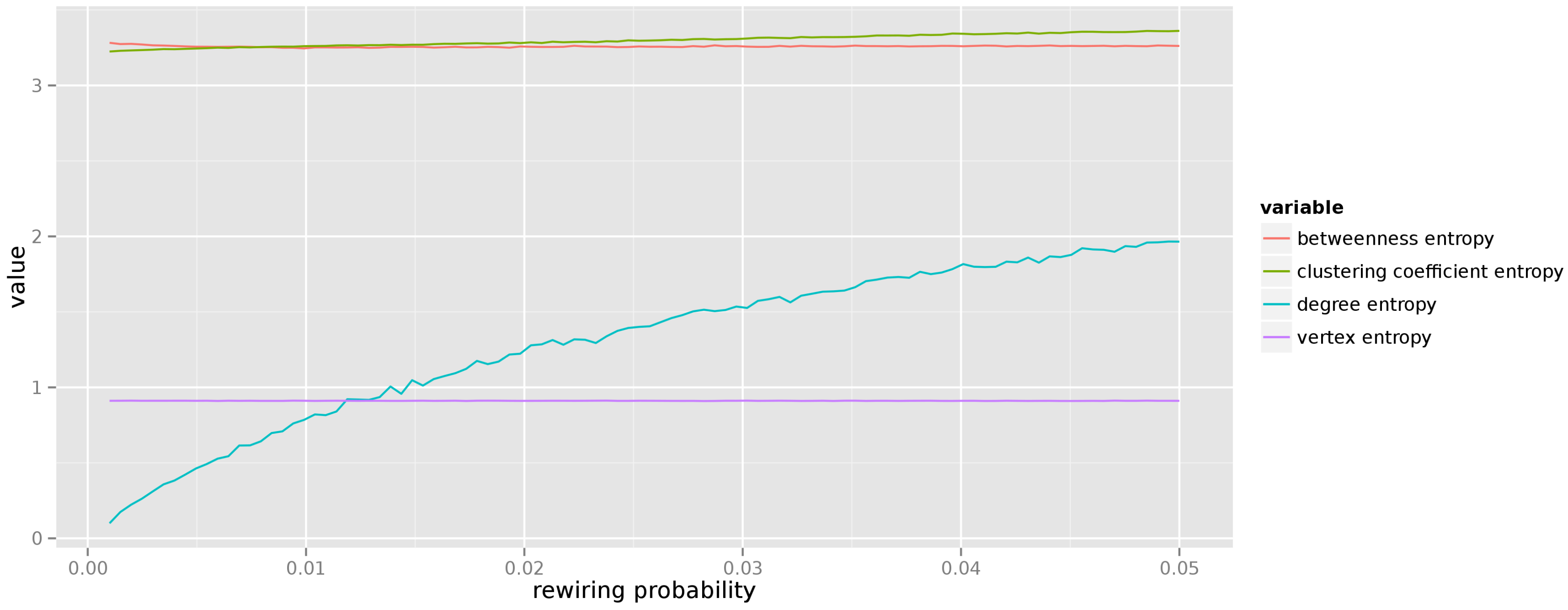
Figure 6 presents the results of a similar experiment conducted for the small world model. Here we have varied the edge rewiring probability from
to
, for a graph with 250 vertices. In the small world model higher values of the rewiring probability introduce more randomness to graph’s structure. The vertex entropy is stable, yet noticeably higher than for the random graph model. Entropies of betweenness and local clustering coefficient distributions remain stable throughout the entire range of varying parameter. Unsurprisingly we observe that the entropy of the degree distribution grows linearly with the increase of the rewiring probability. Indeed, initially all vertices in the graph have equal degrees and no uncertainty about any vertex degree exists, but as the rewiring probability increases, the degrees of individual vertices change in a more random manner, influencing the entropy.
5.1.3. Preferential Attachment
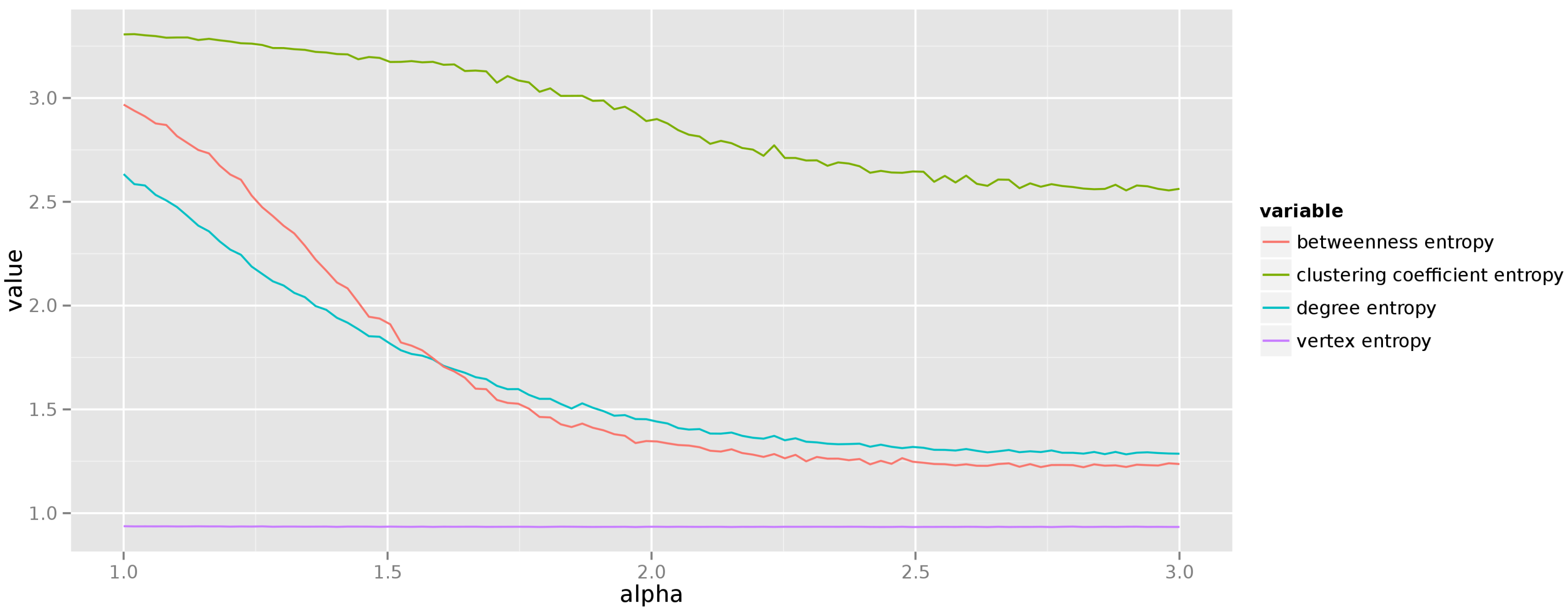
When investigating the preferential attachment model we have decided to change the exponent of the power-law distribution of vertex degrees from 1 to 3, and generate graphs with 250 vertices. The resulting average entropies of centrality measures are presented in
Figure 7. We see that the uncertainty about centrality measure values diminishes with the increasing exponent of the degree distribution. This should come as no surprise as the higher values of the exponent lead to graphs in which preferential attachment creates just a few hubs, and the remaining degree is distributed almost equally among non-hub vertices.
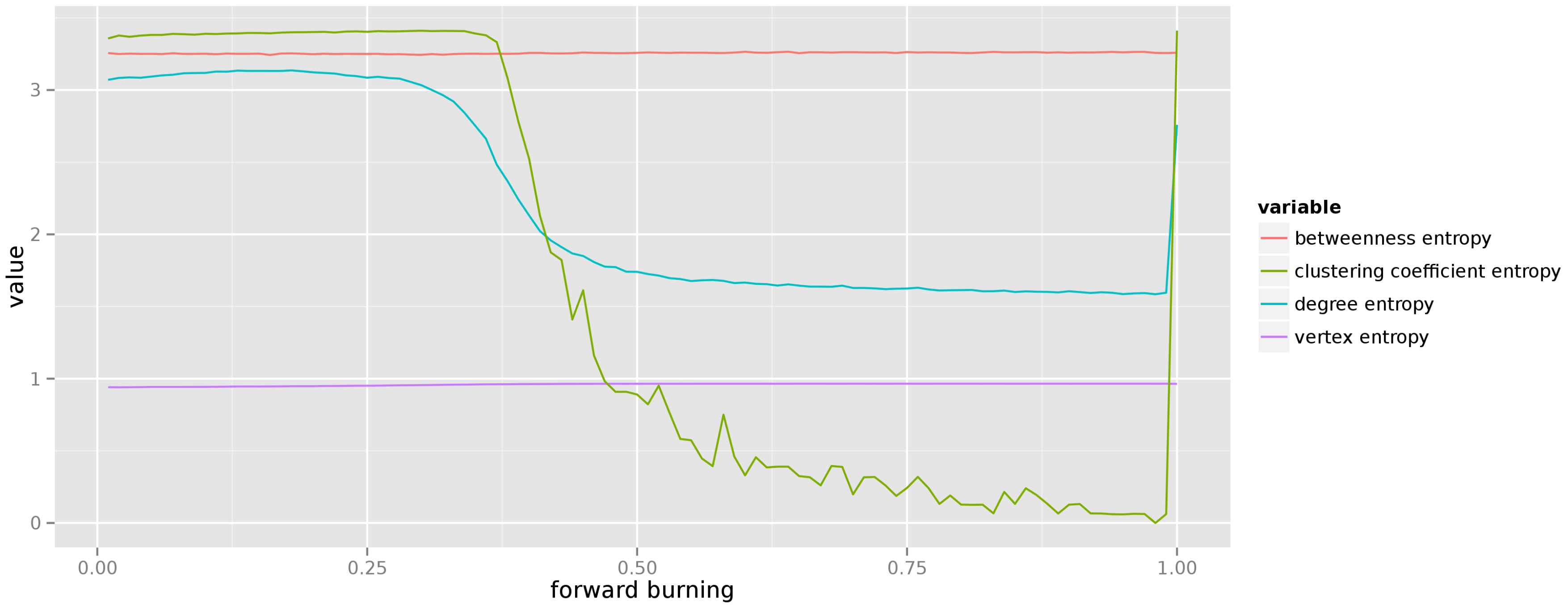
5.1.4. Forest Fire
Finally, for the last theoretical graph model we have varied the forward burning ratio from
to
. The results of measuring the average entropy of centrality measures over 50 different realizations of each graph are depicted in
Figure 8. This result is the most surprising. It remains to be examined why do we observe such sharp drop in the entropy of local clustering coefficient (and, to a lesser extend, of degree). The graph displays high uncertainty about the betweenness of each vertex, but remains quite confident about the expected degree of each vertex.
5.2. k-NN Classification
Next, we proceed to the presentation of the results obtained from running the k-nearest neighbour algorithm to classify graphs. Here we want to verify if features representing the entropy of centrality measures are beneficial for graph comparison and classification. The protocol of the experiment was the following. We have collected detailed statistics from all graphs. Then, we have built the test set of randomly created 1000 graphs, first uniformly choosing the theoretical graph model, and then picking a random parameter value and generating a graph. Finally, we have used the k-nearest neighbour classifier to assign each graph from the test set to one of four classes (random graph, small world, preferential attachment, forest fire). The features used to classify each graph can be divided into two sets: the original features (average degree, average betweenness, average local clustering coefficient), and entropy-related features (average vertex entropy, average entropy of degree distribution, average entropy of betweenness distribution, and average entropy of local clustering coefficient).
When the classifier used only the original features, the accuracy of the classifier was extremely low (
, with the
confidence interval for accuracy of
,
Table 1). Kappa statistic for the accuracy is
which clearly shows that better classification could be achieved by chance alone.
Detailed statistics per class are presented in
Table 2 (A: sensitivity; B: specificity; C: positive predictive value; D: negative predictive value; E: prevalence; F: detection rate; G: detection prevalence; H: balanced accuracy):
Next, we have run the classifier on the full set of features, taking into consideration both original features and the features describing the entropy of centrality measures. This time the accuracy rose to
(
confidence interval
,
), and the confusion matrix is presented in
Table 3. Detailed per class statistics are presented in
Table 4.
Finally, we have decided to test if using entropy-related features alone would improve the accuracy of the classifier. Much to our surprise we have found that these features are far superior to original graph features, resulting in the accuracy of
(
confidence interval
) and
. In particular, the value of the
κ measure suggests that the accuracy of the classifier is much higher than the accuracy which could be attained by chance alone (
p-value for the hypothesis that the accuracy is higher than ”no information rate”, which is basically the accuracy of the majority vote, is 2.2
). However, to obtain such result we had to drop the vertex entropy feature which proved to introduce confusion and lower the results. The final confusion matrix is presented in
Table 5. The detailed per class statistics for entropy features are presented in
Table 6.
The explanation of why entropy-related features work so well is quite straightforward. Centrality measures are being averaged over all vertices in each graph. In fact, most of the theoretical graph models used in our comparison produce graphs, which differ significantly in their structure, but the differences stem primarily from a small subset of significant nodes (hubs), and for a vast majority of vertices their parameters tend to be quite similar across the models. Secondly, the parameters of graphs depend strongly on the particular value of the main parameter of each theoretical graph model. The entropy, on the other hand, is much more stable and better describes the uncertainty of individual vertex properties. Thus, for a model in which resulting vertices may vary significantly regarding their degree or betweenness, the average value of a centrality measure might not be revealing, but the uncertainty about this value is much more descriptive for a given model.
5.3. Comparison of Learners
In order to prove that the usefulness of entropy-related features for graph classification is not limited to the
k-nearest neighbour classifier, we have tested a wide range of different classifiers.
Table 7 presents the results of conducted experiments, the experimental protocol was identical to the protocol used in the previous section. We have used the
R caret package [
31]. Attaining the highest classification accuracy was not the goal of our research, so we have used the default settings of each algorithm, the only change was in the set of features used by each classifier. The classifiers were given either only entropy-related features, only original features, or all available features. We clearly see that almost all classifiers, with the exception of the Naive Bayes classifier, achieve the greatest overall accuracy when working only with entropy-related features, and features pertaining to centrality (average degree, average betweenness, average local clustering coefficient) only tend to confuse the learners.
5.4. Kolmogorov–Smirnov Test
In this section we present the results of the evaluation of the power of the Kolmogorov–Smirnov test to distinguish between different classes of graphs when applied to centrality measure distributions. Let us recall that given two empirical distributions
and
, and their cumulative distribution functions
and
, respectively, the Kolmogorov–Smirnov statistic is given by:
with the null hypothesis stating that
and
come from the same theoretical distribution. The null hypothesis is rejected at
when
, where
are the sizes of
, respectively.
We have tested all theoretical graph models and all centrality measures. The protocol of the experiment was similar to the experiment for k-NN classification. We have generated realizations of each model, with 50 realizations per each value of the main theoretical graph model parameter and three classes of graph sizes (50, 250, and 1000 vertices). Thus, for a given graph size we had 5000 realizations generated for different values of the model parameter.
When comparing an empirical graph with a theoretical graph model, a researcher usually cannot estimate reliably the exact value of the main model parameter. So, one has to compare the empirical distribution of vertex degree, betweenness, and local clustering coefficient with theoretical distributions of these measures for every possible value of the model parameter. In each experiment we have generated 50 graphs, noted their true parameter value, and counted the number of instances for which the Kolmogorov–Smirnov test correctly accepted the null hypothesis. In the following figures the X-axis represents the absolute difference between the empirical parameter value and the theoretical parameter value. For the sake of brevity we will report on the results for a single centrality measure for each theoretical graph model.
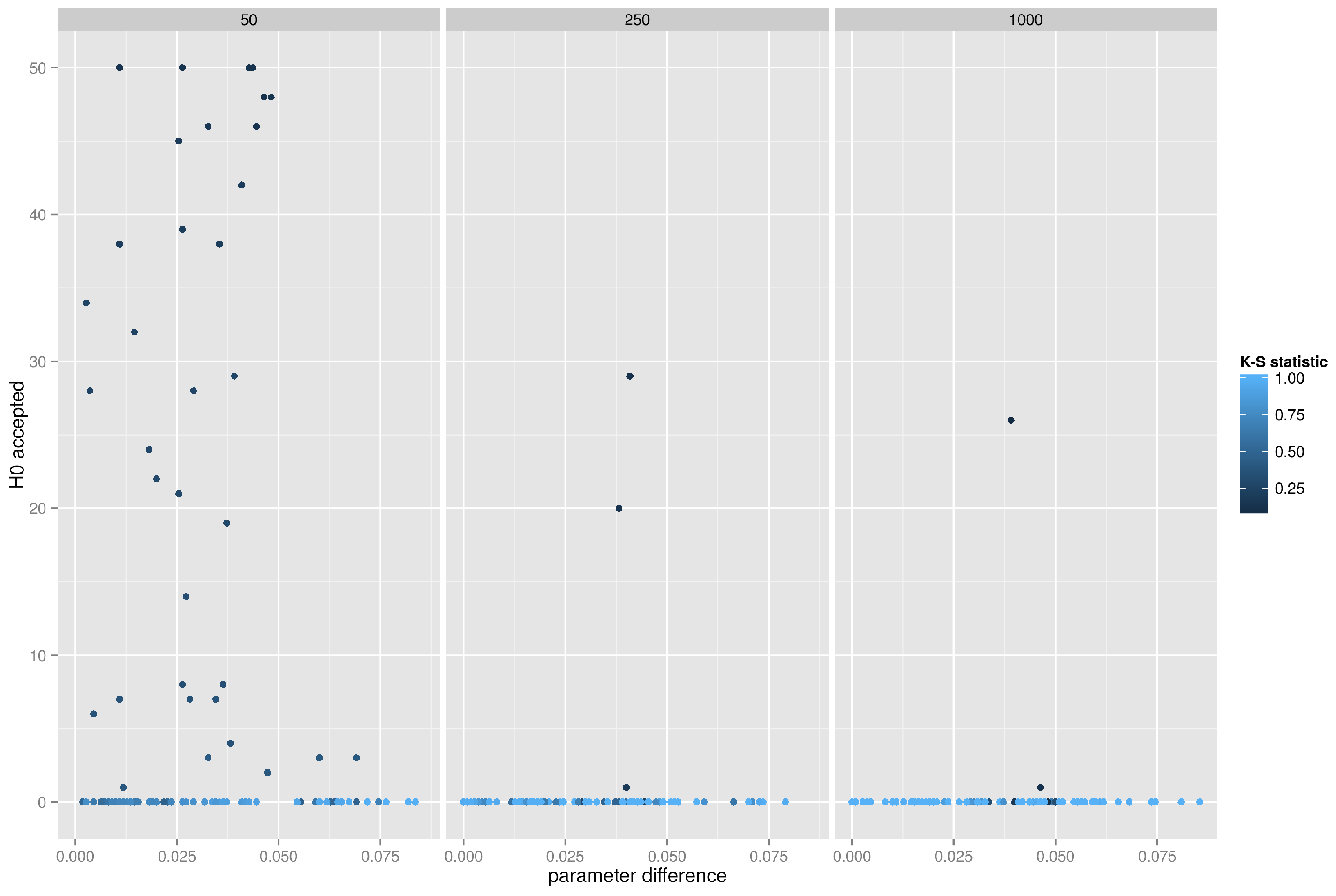
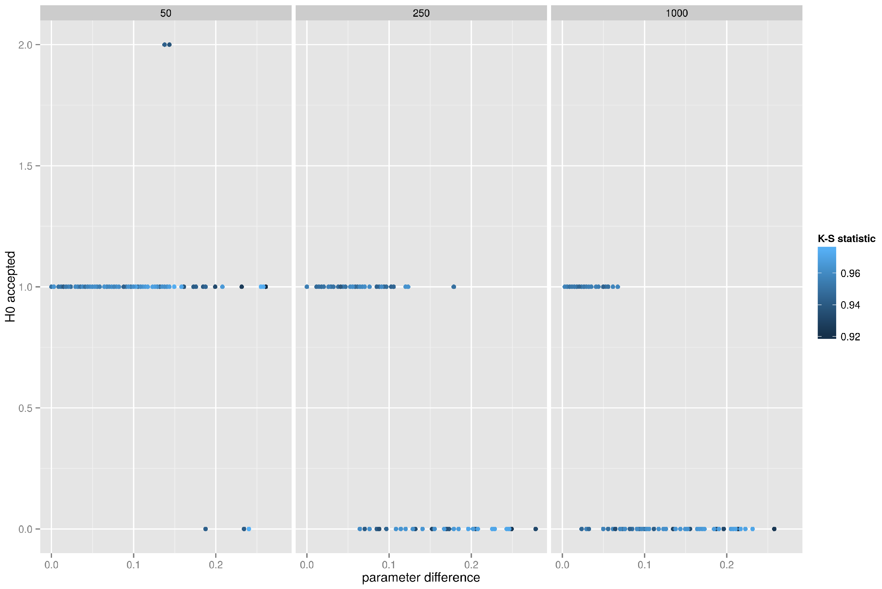
5.4.1. Random Network, K-S Test on the Degree Distribution
Figure 9 presents the accuracy of the K-S test when applied to degree distributions of graphs generated from the random graph model. As can be seen, if the absolute difference between theoretical and empirical edge creation probability is small, not exceeding
, the K-S test correctly accepts many realizations, but only in small networks (with 50 vertices). For networks with 250 or 1000 vertices the test fails miserably and almost always rejects the correct hypothesis.
5.4.2. Small World Network, K-S Test on the Betweenness Distribution
Figure 10 depicts the results of the K-S test of betweenness distributions. More often than not the Kolmogorov–Smirnov test correctly identifies a graph, but with larger graphs it is obvious that the matching can be performed only when the difference in the rewiring probability is small. In other words, given an empirical graph
g one would correctly recognize this graph as belonging to the small world family only if the K-S test was performed on an artificial graph with very similar rewiring probability (for a graph with 1000 vertices the difference in the rewiring probability parameter could not exceed
, otherwise the K-S test would fail to identify the graph
g correctly.
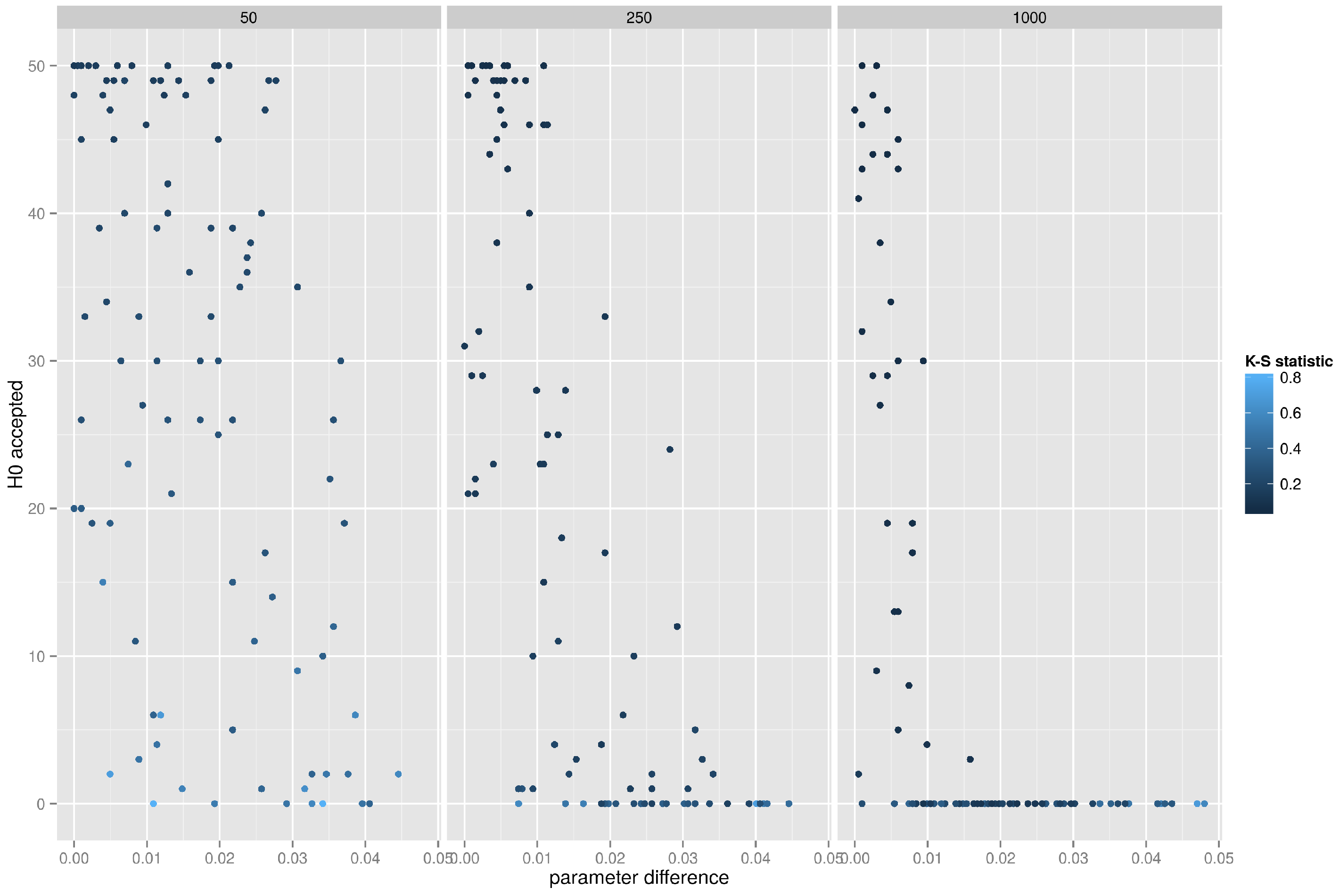
5.4.3. Preferential Attachment Network, K-S Test on the Clustering Coefficient Distribution
The power of the Kolmogorov–Smirnov test to classify graphs originating from the preferential attachment model is presented in
Figure 11. The performance of the test is erratic, it either correctly identifies every graph in the test batch, or it fails to recognize any graph, and this is observed across the entire spectrum of the power law exponent. Interestingly, almost identical behavior is observed when testing the equality of betweenness distributions, but the K-S test completely fails when testing the equality of degree distributions (for each test batch of 50 graphs it accepts at most one graph). This is particularly distressing since the classification of the graph as belonging to the preferential attachment family based solely on the inspection of degree distribution is such a common practice in the scientific community.
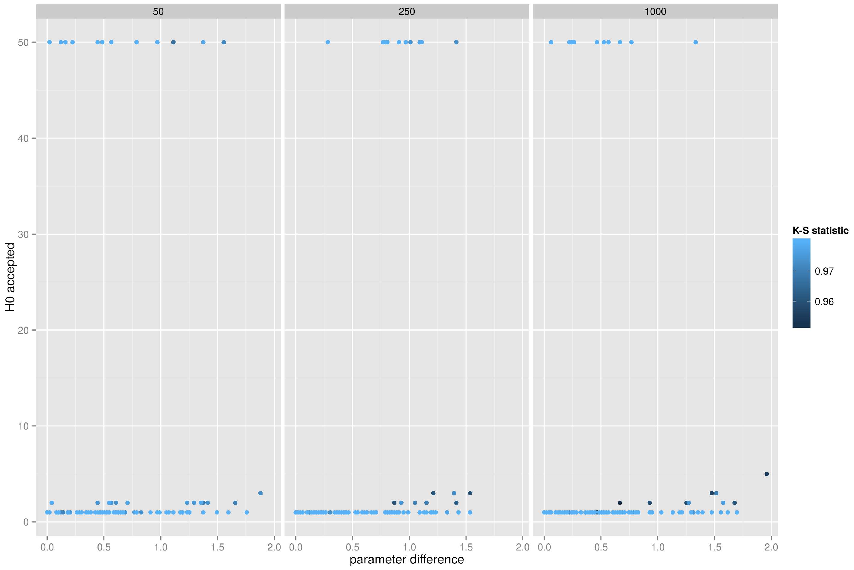
5.4.4. Forest Fire Network, K-S Test on the Degree Distribution
Finally, the results of the Kolmogorov–Smirnov test for the forest fire model are presented in
Figure 12 where degree distributions are compared. Unfortunately, the behavior of the test is very similar to the preferential attachment model—at most 2 graphs out of 50 pass the K-S test at
p-value of
.
6. Conclusions
The work presented in this paper examines the usefulness of entropy when applied to various graph characteristics. We begin by looking at the relationship between centrality measures and their entropies in various theoretical graph models, showing how the uncertainty about the expected value of vertex degree, betweenness, or local clustering coefficient changes with respect to main model parameter. Our goal is to present a set of suggestions on how to correctly assign an empirical graph to one of popular theoretical graph models. To do this, we look at the stability of entropy-related features of a graph, and we investigate the discriminative power of these features for classification. Finally, we examine the power of the Kolmogorov–Smirnov test of cumulative distribution similarity to identify graphs belonging to particular theoretical graph models.
The main conclusions of our up-to-date research can be summarized as follows.
Entropy stability: the most stable are betweenness and clustering coefficient entropies, at least for random graph and small world graph models. For preferential attachment and forest fire models these entropies tend to be more dependent on a particular value of the main model parameter. Degree entropy is unstable across all considered theoretical graph models.
k-NN classification: mean values of centrality measures are very bad descriptors of graphs for the purpose of classification. Adding features representing entropies of these centrality measures improves the performance of the classifier, but using entropy-related features alone produces the most robust classifier.
Kolmogorov–Smirnov test: our tentative conclusion is that the Kolmogorov–Smirnov test of similarity between cumulative distributions cannot be used with confidence to compare graphs. The results of conducted experiments suggest that the discriminative power of the test is not strong enough and that the test fails in most cases to recognize the correct family of a graph.
The research reported in this paper may be under further development. Until now we have experimented only with artificial graphs because we could establish the ground truth (the true theoretical graph model for each graph); thus, we were able to employ classification algorithms. In future we intend to examine a large spectrum of real-world networks and employ both supervised and unsupervised algorithms to group them. The experiments conducted so far found that vertex entropy was both unstable and useless from the point of view of classification. However, we have only examined the vertex entropy computed based on edge weights, and these weights were artificial. In real weighted graphs, vertex entropy could prove to be useful. In order to overcome that the fact that entropy measures adopted in the paper are defined on distributions based on the vertices of a graph it would also be possible to consider more globally defined distributions, e.g., one based on the orbits of the automorphism group or on chromatic properties of a graph. Examination of the classifying power of entropy measures based on these distributions would be an interesting research. Also, we intend to modify the definition of vertex entropy to measure the unexpectedness of vertex degrees in the neighbourhood of a given vertex and verify the usefulness of such measure. Finally, we started first experiments with the algorithmic entropy (also known as the Kolmogorov Complexity) of graphs, but this measure is unfortunately extremely computationally expensive and at this stage we cannot apply it even to small graphs. We are now considering various ways in which the computation of algorithmic complexity could be simplified in order to apply it to real-world graphs.


