Abstract
We propose using five data-driven community detection approaches from social networks to partition the label space in the task of multi-label classification as an alternative to random partitioning into equal subsets as performed by RAkELd. We evaluate modularity-maximizing using fast greedy and leading eigenvector approximations, infomap, walktrap and label propagation algorithms. For this purpose, we propose to construct a label co-occurrence graph (both weighted and unweighted versions) based on training data and perform community detection to partition the label set. Then, each partition constitutes a label space for separate multi-label classification sub-problems. As a result, we obtain an ensemble of multi-label classifiers that jointly covers the whole label space. Based on the binary relevance and label powerset classification methods, we compare community detection methods to label space divisions against random baselines on 12 benchmark datasets over five evaluation measures. We discover that data-driven approaches are more efficient and more likely to outperform RAkELd than binary relevance or label powerset is, in every evaluated measure. For all measures, apart from Hamming loss, data-driven approaches are significantly better than RAkELd (), and at least one data-driven approach is more likely to outperform RAkELd than a priori methods in the case of RAkELd’s best performance. This is the largest RAkELd evaluation published to date with 250 samplings per value for 10 values of RAkELd parameter k on 12 datasets published to date.
1. Introduction
Shannon’s work on the unpredictability of information content inspired a search for the area of multi-label classification that requires more insight: where has the field still been using random approaches to handling data uncertainty when non-random methods could shed light and provide the ability to make better predictions?
Interestingly enough, random methods are prevalent in well-cited and multi-label classification approaches, especially in the problem of label space partitioning, which is a core issue in the problem-transformation approach to multi-label classification.
A great family of multi-label classification methods, called problem transformation approaches, depends on converting an instance of a multi-label classification problem into one or more single-label single-class or multi-class classification problems, performs such classification and then converts the results back to multi-label classification results.
Such a situation stems from the fact that historically, the field of classification started out with solving single-label classification problems; in general, a classification problem of understanding the relationship (function) between a set of objects and a set of categories that should be assigned to it. If the object is allocated to at most one category, the problem is called a single-label classification. When multiple assignments per instance are allowed, we are dealing with a multi-label classification scenario.
In the single-label scenario, in one variant, we deal with a case when there is only one category, i.e., the problem is a binary choice: whether to assign a category or not, such a scenario is called single-class classification, e.g., the case of classifying whether there is a car in the picture or not. The other case is when we have to choose at most one from many possible classes; such a case is called multi-class classification, i.e., classifying a picture with the dominant brand of cars present in it. The multi-label variant of this example would concern classifying a picture with all car brands present in it.
As both single- and multi-class classification problems have been considerably researched during the last few decades, one can naturally see that it is reasonable to transform the multi-label classification case, by dividing the label space, into a single- or a multi-class scenario. A great introduction to the field was written by [1].
The two basic approaches to such a transformation are binary relevance and label powerset. Binary Relevance (BR) takes an a priori assumption that the label space is entirely separable, thus converting the multi-label problem into a family of single-class problems, one for every label, and making a decision whether to apply it or not. Converting the results back to multi-label classification is based just on taking a union of all assigned labels. Regarding our example, binary relevance assumes that correlations between car brands are not important enough and discards them a priori by classifying with each brand separately.
Label Powerset (LP) makes an opposite a priori assumption: the label space is non-divisible label-wise, and each possible label combination becomes a unique class. Such an approach yields a multi-class classification problem on a set of classes equal to the powerset of the label set, i.e., growing exponentially if one treats all label combinations as possible. In practice, this would be intractable. Thus, as [2] note, label powerset is most commonly implemented to handle only these combinations of classes that occur in the training set and, as such, is prone to overfitting. It is also, per [3], prone to differences in label combination distributions between the training set and the test set, as well as to an imbalance in how label combinations are distributed in general.
To remedy the overfitting of label powerset, Tsoumakas et al. [3] propose to divide the label space into smaller subspaces and use label powerset in these subspaces. The source of proposed improvements come from the fact that it should be easier for label powerset to handle a large number of label space combinations in a smaller space. Two proposed approaches are called random k-label sets (RAkEL). RAkEL comes in two variants: a label space partitioning RAkELd, which divides the label set into k disjoint subsets, and RAkELo, which is a sampling approach that allows overlapping of label subspaces. In our example, RAkEL would randomly select a subset of brands and use the label powerset approach for brand combinations in all of the subspaces.
While these methods were developed, we saw advances in other fields that brought us more and more tools to explore relations between entities in data. Social and complex networks have been flourishing after most of the well-established methods were published. In this paper, we propose a data-driven approach for label space partitioning in multi-label classification. While we tackle the problem of classification, our goal is to spark a reflection on how data-driven approaches to machine learning using new methods from complex/social networks can improve established procedures. We show that this direction is worth pursuing, by comparing method-driven and data-driven approaches towards partitioning the label space.
Why should one rely on label space division at random? Should not a data-driven approach be better than random choice? Are methods that perform simplistic a priori assumptions truly worse than the random approach? What are the variances of result quality upon label space partitioning? Instead of selecting random subspaces of brands, we could consider that some city brands occur more often with each other and less so with other suburban brands. Based on such a premise, we could build a weighted graph depicting the frequency of how often two brands occur together in photos. Then, using well-established community detection methods on this graph, we could provide a data-driven partition for the label space.
In this paper, we wish to follow Shannon’s ambition to search for a data-driven solution, an approach of finding structure instead of accepting uncertainty. We run RAkELd on 12 benchmark datasets, with different values of parameter k, taking k to be equal to 10%, 20%, …, 90% of the label set size. We draw 250 distinct partitions of the label set into subsets of k labels, per every value of k. In case there are less than 250 possible partitions of the label space (e.g., because there are less than 10 labels), we consider all possible partitions. We then compare these results against the performance of methods based both on a priori assumptions—binary relevance and label powerset—and also well-established community detection methods employed in social and complex network analysis to detect patterns in the label space. For each of the measures, we state three hypotheses:
- RH1:
- a data-driven approach performs statistically better than the average random baseline;
- RH2:
- a data-driven approach is more likely to outperform RAkELd than methods based on a priori assumptions;
- RH3:
- a data-driven approach has a higher likelihood to outperform RAkELd in the worst case than methods based on a priori assumptions;
- RH4:
- a data-driven approach is more likely to perform better than RAkELd, than otherwise, i.e., the worst-case likelihood is greater than ;
- RH5:
- the data-driven approach is more time efficient than RAkELd.
We describe the multi-label classification problem and existing methods in Section 3, our new proposed data-driven approach in Section 4 and compare the results of the likelihood of a data-driven approach being better than randomness in Section 6. We provide the technical detail of the experimental scenario in Section 5. We conclude with the main findings of the paper and future work in Section 7.
2. Related Work
Our study builds on two kinds of approaches to multi-label classification: problem transformation and ensemble. We extend the label powerset problem transformation method by employing an ensemble of classifiers to classify obtained partitions of the label space separately. We show that partitioning the label space randomly, as is done in the RAkEL approach, can be improved by using a variety of methods to infer the structure of partitions from the training. We extend the original evaluation of random k-label sets’ performance using a larger sampling of the label space and providing deeper insight into how RAkELd performs. We also provide some insights into the nature of random label space partitioning in RAkELd. Finally, we provide alternatives to random label space partitioning that are very likely to yield better results than RAkELd depending on the selected measure, and we show which methods to use depending on the generalization strategy.
The classifier chains [4] approach to label space partitioning is based on a Bayesian conditioning scheme, in which labels are ordered in a chain, and then, the n-th classification is performed taking into account the output of the last classifications. These methods suffer from a variety of challenges: the results are not stable when ordering of labels in the chain changes, and finding the optimal chain is NP-hard. Existing methods that optimize towards best quality cannot handle more than 15 labels in a dataset (e.g., Bayes-optimal Probabilistic Classifier Chains (PCC) [5]). Furthermore, in every classifier chain approach, one always needs to train at least the same number of classifiers as there are labels and if ensemble approaches are applied, much more. In our approach, we use community detection methods to divide the label space into a fewer number of cases to classify as multi-class problems, instead of transforming to a large number of single-class problems that are interdependent. We also do not strive to find the directly optimal solution to community detection problems on the label co-occurrence graph, to avoid overfitting; instead, we perform approximations of the optimal solutions. This approach provides a large overhead over random approaches. We note that it would be an interesting question whether the random orderings in classifier chains are as suboptimal of a solution, as random partitioning turns out to be in label space partitioning. Yet, it is not the subject of the study and is open to further research.
Tsoumakas et al.’s [6] Hierarchy Of Multilabel classifiERs (HOMER) is a method of two-step hierarchical multi-label classification in which the label space is divided based on label assignment vectors; then, observations are classified first with cluster meta-labels; and finally, for each cluster they were labeled with, they are classified with labels of that cluster. We do not compare to HOMER directly in this article, due to the different nature of the classification scheme, as the subject of this study is to evaluate how data-driven label space partitioning using complex/social network methods, which can be seen as weak classifiers (as all objects are assigned automatically to all subsets), can improve the random partitioning multi-label classification. HOMER uses a strong classifier to decide which object should be classified in which subspace. Although we do not compare directly to HOMER, due to the difference in the classification scheme and base classifier, our research shows similarities to Tsoumakas’s result that abandoning random label space partitioning for the k-means-based data-driven approach improves classification results. Thus, our results are in accord, yet we provide a much wider study, as we have performed a much larger sampling of the random space than the authors of HOMER in their method-describing paper.
Madjarov et al. [7] compare the performance of 12 multi-label classifiers on 11 benchmark sets evaluated by 16 measures. To provide statistical support, they use a Friedman multiple comparison procedure with a post hoc Nemenyi test. They include the RAkELo procedure in their study, i.e., the random label subsetting instead of partitioning. They do not evaluate the partitioning strategy RAkELd, which is the main subject of this study. Our main contribution, the study of how RAkELd performs against more informed approaches, therefore fills the unexplored space of Madjarov et al.’s extensive comparison. Note that, due to computational limits, we use Classification and Regression Trees (CART) instead of Support Vector Machines (SVM) as the single-label base classifier, as explained in Section 5.2.
Zhang et al. [8] review theoretical aspects and reported the experimental performance of eight multi-label algorithms and categorize them by the order of correlations taken into account and the evaluation measure that they try to optimize.
3. Multi-Label Classification
In this section, we aim to provide a more rigid description of the methods we use in the experimental scenario. We start by formalizing the notion of classification. Classification aims to understand a phenomenon, a relationship (function ) between objects and categories, by generalizing from empirically-collected data D:
- objects are represented as feature vectors from the input space X;
- categories, i.e., labels or classes come from a set L, and it spans the output space Y:
- –
- in the case of single-label single-class classification, and
- –
- in the case of single-label multi-class classification, and
- –
- in the case of multi-label classification,
- the empirical evidence collected: ;
- a quality criterion function q.
In practice the empirical evidence D is split into two groups: the training set for learning the classifier and the test set to use for evaluating the quality of classifier performance. For the purpose of this section, we will denote as the training set.
The goal of classification is to learn a classifier , such that h generalizes in a way that maximizes q.
We are focusing on problem-transformation approaches that perform multi-label classification by transforming it to a single-label classification and convert the results back to the multi-label case. In this paper, we use CART decision trees as the single-label base classifier. CART decision trees are a single-label classification method capable of both single- and multi-class classification. A decision tree constructs a binary tree in which every node performs a split based on the value of a chosen feature from the feature space X. For every feature, a threshold is found that minimizes an impurity function calculated for a threshold on the data available in the current node’s subtree. For the selected pair of a feature and a threshold θ, a new split is performed in the current node. Objects with values of the feature lesser than θ are evaluated in the left subtree of the node, while the rest in the right. The process is repeated recursively for every new node in the binary tree until the depth limit selected for the method is reached or there is just one observation left to evaluate. In all of our scenarios, we use CART as the base single-label single- and multi-class base classifier.
Binary relevance learns single-label single-class base classifiers for each and outputs the multi-label classification using a classifier .
Label powerset constructs a bijection between each subset of labels and a class . Label powerset then learns a single-label multi-class base classifier and transforms its output into a multi-label classification result .
RAkELd performs a random partition of the label set L into k subsets . For each , a label powerset classifier is learned. For a given input vector , the RAkELd classifier h performs multi-label classification with each classifier and then sums the results, which can be formally described as . Following the RAkELd scenario from [3], all partitions of the set L into k subsets are equally probable.
4. The Data-Driven Approach
Having described the baseline random scenario of RAkELd, we now turn to explaining how complex/social network community detection methods fit into a data-driven perspective for label space division. In this scenario, we are transforming the problem exactly like RAkELd, but instead of performing random space partitioning, we construct a label co-occurrence graph from the training data and perform community detection on this graph to obtain a label space division.
4.1. Label Co-Occurrence Graph
We construct the label co-occurrence graph as follows. We start with an undirected co-occurrence graph G with the label set L as the vertex set and the set of edges constructed from all pairs of labels that were assigned together at least once to an input object in the training set (here, denote labels, i.e., elements of the set L):
One can also extend this unweighted graph G to a weighted graph by defining a function :
Using such a graph G, weighted or unweighted, we find a label space division by using one of the following community detection methods to partition the graph’s vertex set, which is equal to the label set.
4.2. Dividing the Label Space
Community detection methods are based on different principles as different fields defined communities differently. We are employing a variety of methods.
Modularity-based approaches, such as the fast greedy [9] and the spectral leading eigenvector algorithms, are based on detecting a partition of label sets that maximizes the modularity measure by [10]. Behind this measure lies an assumption that true community structure in a network corresponds to a statistically-surprising arrangement of edges [10], i.e., that a community structure in a real phenomenon should exhibit a structure different from an average case of a random graph, which is generated under a given null model. A well-established null model is the configuration model, which joins vertices together at random, but maintains the degree distribution of vertices in the graph.
For a given partition of the label set, the modularity measure is the difference between how many edges of the empirically-observed graph have both ends inside of a given community, i.e., versus how many edges starting in this community would end in a different one in the random case: . More formally, this is . In the case of weights, instead of counting the number of edges, the total weight of edges is used, and instead of taking vertex degrees in r, the vertex strengths are used; a precise description of weighted modularity can be found in Newman’s paper [11].
Finding is NP-hard, as shown by Brandes et al. [12]. We thus employ three different approximation-based techniques instead: a greedy, a multi-level hierarchical and a spectral recursively-dividing algorithm.
The fast greedy approach works based on greedy aggregation of communities, starting with singletons and merging the communities iteratively. In each iteration, the algorithm merges two communities based on which merge achieves the highest contribution to modularity. The algorithm stops when there is no possible merge that would increase the value of the current partition’s modularity. Its complexity is .
The leading eigenvector approximation method depends on calculating a modularity matrix for a split of the graph into two communities. Such a matrix allows one to rewrite the two-community definition of modularity in a matrix form that can be then maximized using the largest positive eigenvalue and signs of the corresponding elements in the eigenvector of the modularity matrix: negative ones assigned to one community, positive ones to another. The algorithm starts with all labels in one community and performs consecutive splits recursively until all elements of the eigenvector have the same sign or the community is a singleton. The method is based on the simplest variant of spectral modularity approximation as proposed by Newman [13]. Its complexity is .
The infomap algorithm concentrates on finding the community structure of the network with respect to flow and to exploit the inference-compression duality to do so [14]. It relies on finding a partition of the vertex set that minimizes the map equation. The map equation divides flows through the graph into intra-community ones and the between-community ones and takes into consideration an entropy-based frequency-weighted average length of codewords used to label nodes in communities and inter-communities. Its complexity is .
The label propagation algorithm [15] assigns a unique tag to every vertex in the graph. Next, it iteratively updates the tag of every vertex with the tag assigned to the majority of the elements’ neighbors. The updating order is randomly selected at each iteration. The algorithm stops when all vertices have tags that are in accord with the dominant tag in their neighborhood. Its complexity is .
The walktrap algorithm is based on the intuition that random walks on a graph tend to get “trapped” into densely-connected parts corresponding to communities [16]. It starts with a set of singleton communities and agglomerates obtained communities in a greedy iterative approach based on how close two vertices are in terms of random-walk distance. More precisely, each step merges two communities to maximize the decrease of the mean (averaged over vertices) of squared distances between a vertex and all of the vertices that are in the vertex’s community. The random walk distance between two nodes is measured as the distance between the random walk probability distribution starting in each of the nodes. The distances are of the same maximum length provided as a parameter to the method. Its expected complexity is .
In complexity notation, N is the number of nodes and M the number of edges.
4.3. Classification Scheme
In our data-driven scheme, the training phase is performed as follows:
- the label co-occurrence graph is constructed based on the training dataset;
- the selected community detection algorithm is executed on the label co-occurrence graph;
- for every community , a new training dataset is created by taking the original input space with only the label columns that are present in ;
- for every community, a classifier is learned on training set .
The classification phase is performed by performing classification on all subspaces detected in the training phase and taking the union of assigned labels: .
5. Experiments and Materials
To prepare the ground for results, in this section, we describe which datasets we have selected for evaluation and why. Then, we present and justify model selection decisions for our experimental scheme. Next, we describe the configuration of our experimental environment. Finally, we describe the measures used for evaluation.
5.1. Datasets
Following Madjarov’s study [7], we have selected 12 different well-cited multi-label classification benchmark datasets. The basic statistics of datasets used in experiments, such as the number of data instances, the number of attributes, the number of labels, the labels’ cardinality, density and the distinct number of label combinations, are available online [17]. We selected the datasets to obtain a balanced representation of problems in terms of the number of objects, the number of labels and domains. At the moment of publishing, this is one of the largest studies of RAkELd, both in terms of datasets examined and in terms of random label partitioning sample count. This study also exhibits a higher ratio of the number of datasets to the number of methods than other studies.
The text domain is represented by 5 datasets: bibtex, delicious, enron, medical and tmc2007-500. Bibtex [18] comes from the ECML/PKDD 2008 Discovery Challenge and is based on data from the Bibsonomy.org publication sharing and bookmarking website. It exemplifies the problem of assigning tags to publications represented as an input space of bibliographic metadata, such as: authors, paper/book title, journal volume, etc. Delicious [6] is another user-tagged dataset. It spans over 983 labels obtained by scraping the 140 most popular tags from the del.icio.us bookmarking website, retrieving the 1000 most recent bookmarks, selecting the 200 most popular, deduplication and filtering tags that were used to tag less than 10 websites. For those labels, websites tagged with them were scraped, and from their contents, the top 500 words ranked by the method were selected as input features. Tmc2007-500 [6] contains an input space consisting of the similarly selected top 500 words appearing in flight safety reports. The labels represent the problems being described in these reports. Enron [19] contains emails from senior Enron Corporation employees categorized into topics by the UC Berkeley Enron E-mail Analysis Project [20] with the input space being a bag of word representation of the e-mails. The Medical [4] dataset is from the Medical Natural Language Processing Challenge [21]. The input space is a bag-of-words representation of patient symptom history, and labels represent diseases following the International Classification of Diseases.
The multimedia domain consists of five datasets: scene, corel5k, mediamill, emotions and birds. The image dataset scene [22] semantically indexes still scenes annotated with any of the following categories: beach, fall-foliage, field, mountain, sunset and urban. The birds dataset [23] represents a problem of matching bird voice recordings’ extracted features with a subset of 19 bird species that are present in the recording; each label represents one species. This dataset was introduced [24] during the The 9th Annual MLSP competition. A larger image set corel5k [25] contains normalized-cut segmented images clustered into 499 bins. The bins were labeled with 374 subset labels. The mediamill dataset of annotated video segments [26] was introduced during the 2005 NIST TRECVID challenge [27]. It is annotated with 101 labels referring to elements observable in the video. The emotions dataset [28] represents the problem of the automated detection of emotion in music, assigning a subset of music emotions based on the Tellegen–Watson–Clark model to each of the songs.
The biological domain is represented with two datasets: yeast and genbase. The yeast [29] dataset concerns the problem of assigning functional classes to genes of the Saccharomyces cerevisiae genome. The genbase [30] dataset represents the problem of assigning classes to proteins based on detected motifs that serve as input features.
5.2. Experiment Design
Using 12 benchmark datasets evaluated with five performance measures, we compare eight approaches to label space partitioning for multi-label classification:
- five methods that divide the label space based on structure inferred from the training data via label co-occurrence graphs, in both unweighted and weighted versions of the graphs;
- two methods that take an a priori assumption about the nature of the label space: binary relevance and label powerset;
- one random label space partitioning approach that draws partitions with equal probability: RAkELd.
In the random baseline (RAkELd), we perform 250 samplings of random label space partitions into k-label subsets for each evaluated value of k. If a dataset had more than 10 labels, we took values of k ranging from 10% to 90% with a step of 10%, rounding to the closest integer number if necessary. In case of two datasets with a smaller number of labels, i.e., scene and emotions, we evaluated RAkELd for all possible label space partitions due to their low number. The number of label space division samples per dataset can be found in Appendix A (Table A1).
As no one knows the true distribution of classification quality over label space partitions, we have decided to use a large number of samples, 250 per each of the groups, 2500 altogether, to get as close to a representative sample of the population as was possible with our infrastructure limitations.
As the base classifier, we use CART decision trees. While we recognize that the majority of studies prefer to use SVMs, we note that it is intractable to evaluate nearly 32,500 samples of the random label space partitions using SVMs. We have thus decided to use a classifier that presents a reasonable trade-off between quality and computational speed.
We perform statistical evaluation of our approaches by comparing them to average performance of the random baseline of RAkELd. We average RAkELd results per dataset, which is justified by the fact that this is the expected result one would get without performing extensive parameter optimization. Following Derrac et al.’s [31] de facto standard modus operandi, we use the Friedman test with Iman–Davenport modifications to detect differences between methods, and we check whether a given method is statistically better than the average random baseline using Rom’s post-hoc pairwise test. We use these tests’ results to confirm or reject RH1.
We do not perform statistical evaluation per group (i.e., isolating each value of k from 10% to 90%) due to the lack of non-parametric repeated measure tests, as noted by Demsar in the classic paper [32].
Instead, to account for variation, we consider the probability that a given data-driven approach to label space division is better than random partitioning. These probabilities were calculated per dataset, as the fraction of random outputs that yielded worse results than a given method. Thus, for example, if infomap has a 96.5% probability of having higher better subset accuracy (SA) than the random approach in Corel5k, this means that on this dataset, infomap’s SA score was better than the scores achieved by 96.5% of all RAkELd experiments. We check the median, the mean and the minimal (i.e., worst case) likelihoods. We use these results to confirm or reject RH2, RH3 and RH4.
5.3. Environment
We used scikit-multilearn (Version 0.0.1) [33], a scikit-learn API compatible library for multi-label classification in python that provides its own implementation of several classifiers and uses scikit-learn [34] multi-class classification methods. All of the datasets come from the MULAN [35] dataset library [17] and follow MULAN’s division into the train and test subsets.
We use CART decision trees from the scikit-learn package (Version 0.15), with the Gini index as the impurity function. We employ community detection methods from the Python version of the igraph library [36] for both weighted and unweighted graphs. The performance measures’ implementation comes from the scikit-learn metrics package.
5.4. Evaluation Methods
Following Madjarov et al.’s [7] taxonomy of multi-label classification evaluation measures, we use three example-based measures: Hamming loss, subset accuracy and Jaccard similarity, as well as a label-based measure, F1, as evaluated by two averaging schemes: micro and macro. The following definitions are used:
- X is the set of objects used in the testing scenario for evaluation
- L is the set of labels that spans the output space Y;
- denotes an example object undergoing classification;
- denotes the label set assigned to object by the evaluated classifier h;
- y denotes the set of true labels for the observation ;
- , , , are respectively true positives, false positives, false negatives and true negatives of the of label , counted per label over the output of classifier h on the set of testing objects , i.e., ;
- the operator converts the logical value to a number, i.e., it yields 1 if p is true and 0 if p is false.
5.4.1. Example-Based Evaluation Methods
Hamming loss is a label-wise decomposable function counting the fraction of labels that were misclassified. ⊗ is the logical exclusive or.
The accuracy score and subset 0/1 loss are instance-wise measures that count the fraction of input observations that have been classified exactly the same as in the golden truth.
Jaccard similarity is a measure of the size of similarity between the prediction and the ground truth comparing what is the cardinality of an intersection of the two, compared to the union of the two. In other words, what fraction of all labels taken into account by any of the prediction or ground truth were assigned to the observation in both of the cases.
5.4.2. Label-Based Evaluation Methods
The F1 measure is a harmonic mean of precision and recall where none of the two are more preferred than the other. Precision is the measure of how much the method is immune to Type I error, i.e., falsely classifying negative cases as positives: false positives or FP. It is the fraction of correctly positively-classified cases (i.e., true positives) to all positively-classified cases. It can be interpreted as the probability that an object without a given label will not be labeled as having it. Recall is the measure of how much the method is immune to the Type II error, i.e., falsely classifying positive cases as negatives: false negatives or FN. It is the fraction of correctly positively-classified cases (i.e., true positives) to all positively-classified label. It can be interpreted as the probability that an object with a given label will be labeled as such.
These measures can be averaged from two perspectives that are not equivalent in practice due to a natural non-uniformity of the distribution of labels among input objects in any testing set. Two averaging techniques are well-established, as noted by [37].
Micro-averaging gives equal weight to every input object and performs a global aggregation of true/false positives/negatives, averaging over all objects first. Thus:
In macro-averaging, the measure is first calculated per label, then averaged over the number of labels. Macro averaging thus gives equal weight to each label, regardless of how often the label appears.
6. Results and Discussion
We describe the performance per measure first and then look at how methods behave across measures. We evaluate each of the research hypotheses, RH1 to RH4, for each of the measures. We then look at how these methods performed across datasets. We compare the median and the mean of the achieved probabilities to assess the average advantage over randomness; the higher the better. We compare the median and the means, as in some cases, the methods admit a single worst-performing outlier, while in general providing a great advantage over random approaches. We also check how each method performs in the worst case, i.e., what is the minimum probability of it being better than randomness in label space division?
6.1. Micro-Averaged F1 Score
When it comes to ranking of how well methods performed in micro-averaged F1, fast greedy and walktrap approaches used on a weighted label co-occurrence graph performed best, followed by BR, leading eigenvector and unweighted walktrap/modularity-maximizations methods. Furthermore, weighted label propagation and infomap were statistically significantly better than the average random performance. We confirm RH1, with evidence presented in Figure 1 and Figure 2 and Table 1.
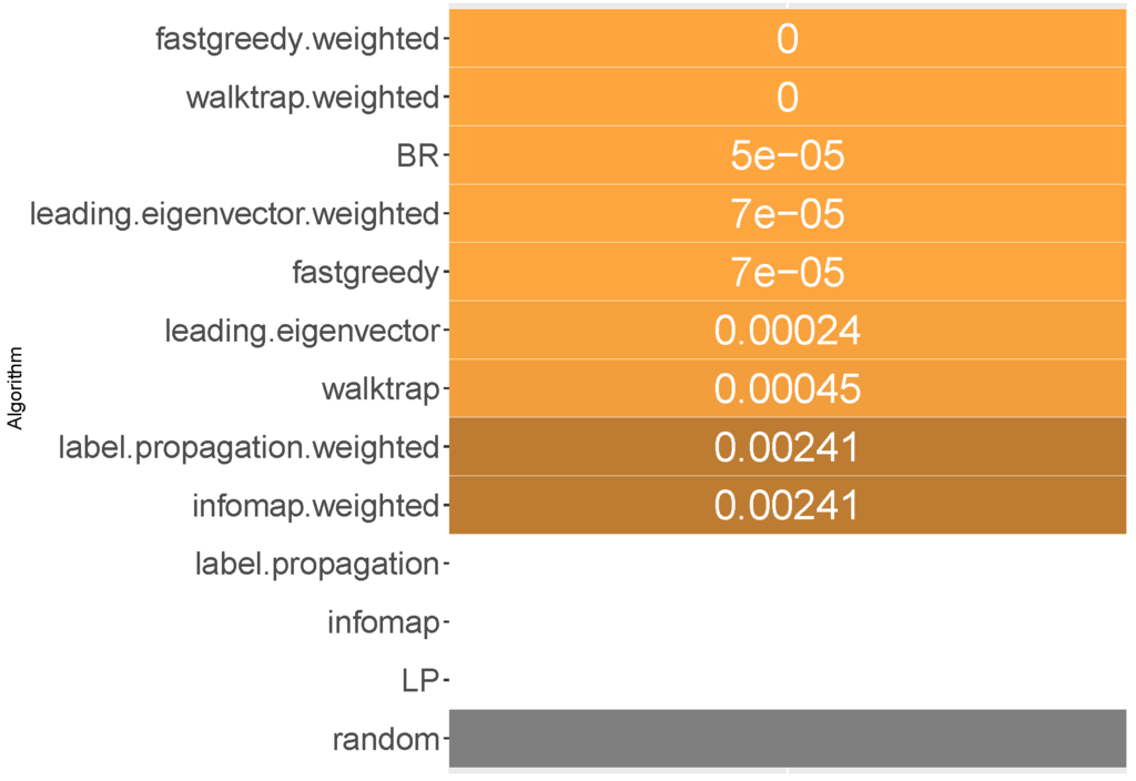
Figure 1.
Statistical evaluation of the method’s performance in terms of micro-averaged F1 score. Gray, baseline; white, statistically identical to the baseline; otherwise, the p-value of the hypothesis that a method performs better than the baseline.
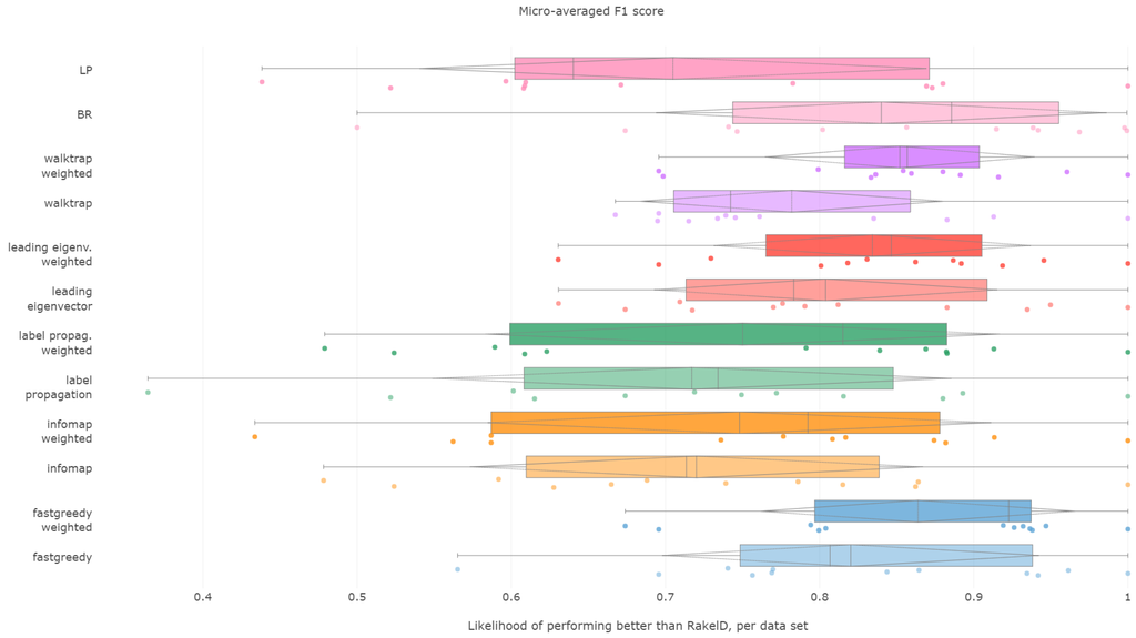
Figure 2.
Histogram of the methods’ likelihood of performing better than RAkELd in the micro-averaged F1 score aggregated over datasets.

Table 1.
Likelihood of performing better than RAkELd in the micro-averaged F1 score of every method for each dataset.
In terms of the micro-averaged F1, the weighted fast greedy approach has both the highest mean (86%) and median (92%) likelihood of scoring better than random baseline. Binary relevance and weighted variants of walktrap, leading eigenvector also performed well with a mean likelihood of 83% to 85% and a lower, but still satisfactory median of 85% to 88%. We confirm RH2.
Modularity-based approaches also turn out to be most resilient. The weighted variant of walktrap was the most resilient with a 69.5% likelihood in the worst case, followed closely by a weighted fast greedy approach with 67% and unweighted walktrap with 66.7%. We note that, apart from a single outlying datasets, all methods (apart from label powerset) had better than 50% likelihood of performing better than RAkELd. Binary relevance’s worst case likelihood was exactly . We thus confirm both RH3 and RH4.
Fast greedy and walktrap weighted approaches yielded the best advantage over RAkELd, both in the average and worst cases. Binary relevance also provided a strong overhead against random label space division, while achieving just in the worst case scenario. Thus, when it comes to micro-averaged F1 scores, RAkELd random approaches to label space partitions should be dropped in favor of weighted fast greedy and walktrap methods or binary relevance. All of these methods are also statistically significantly better than the average random baseline. We therefore confirm RH1, RH2, RH3 and RH4 for micro-averaged F1 scores.
We also note that RAkELd was better than label powerset on micro-averaged F1 in 57% of the cases in the worst case, while Tsoumakas et al.’s original paper [3] provides argumentation of micro-F1 improvements over LP yielded by RAkELd, using SVMs. We note that our observation is not contrary: LP failed to produce significantly different results than the average random baseline in our setting. Instead, our results are complementary, as we use a different classifier, but the intuition can be used to comment on Tsoumakas et al.’s results. While in some cases, RAkELd provides an improvement over LP in F1 score, on average, the probability of drawing a random subspace better is only 30%. We still note that it is much better to use one of the recommended community detection-based approaches instead of a method based on a priori assumptions.
6.2. Macro-Averaged F1 Score
All methods, apart from unweighted label propagation and infomap, performed significantly better than the average random baseline. The highest ranks were achieved by weighted fast greedy, binary relevance and unweighted fast greedy. We confirm RH1, with evidence presented in Figure 3 and Figure 4 and Table 2.
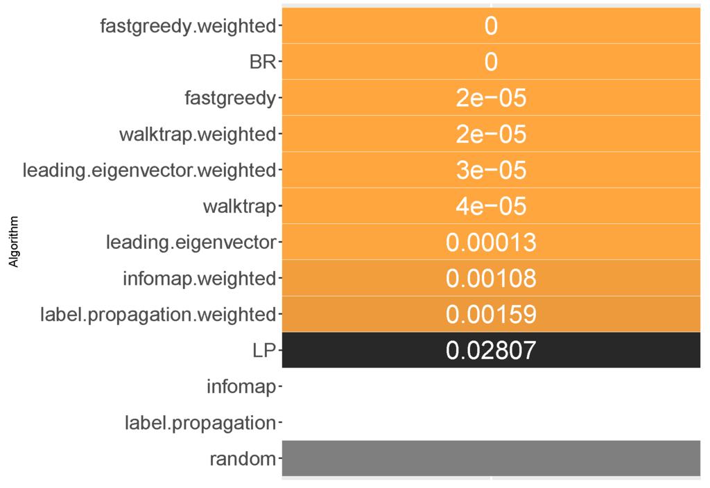
Figure 3.
Statistical evaluation of the method’s performance in terms of macro-averaged F1 score. Gray, baseline; white, statistically identical to baseline; otherwise, the p-value of the hypothesis that a method performs better than the baseline.
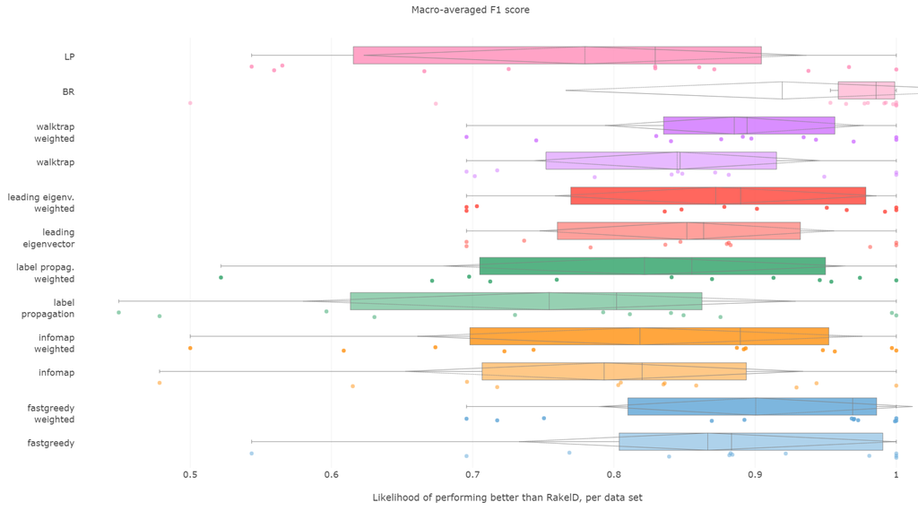
Figure 4.
Histogram of the methods’ likelihood of performing better than RAkELd in the macro-averaged F1 score aggregated over datasets.
Table 2.
Likelihood of performing better than RAkELd in the macro-averaged F1 score of every method for each dataset.
Fast greedy and walktrap approaches used on the weighted label co-occurrence graph were most likely to perform better than RAkELd samples, followed by BR, leading eigenvector and unweighted walktrap/modularity-maximizations methods. Furthermore, weighted label propagation and infomap were statistically significantly better than the average random performance.
Binary relevance and weighted fast greedy were the two approaches that surpassed the 90% likelihood of being better than random label space divisions in both the median (98.5% and 97%, respectively) and mean (92% and 90%) cases. Weighted walktrap and leading eigenvector followed closely with both the median and the mean likelihood of 87% to 89%. We thus reject RH2, as binary relevance achieved greater likelihoods than the best data-driven approach.
When it comes to resilience, all modularity (apart from unweighted fast greedy) methods achieve the same high worst-case 70% probability of performing better than RAkELd. Binary relevance underperformed in the worst case, being better exactly in 50% of the cases. All methods on all datasets, apart from the outlier case of infomap’s and label propagation’s performance on the scene dataset, are likely to yield a better macro-averaged F1 score than the random approaches. We confirm RH3 and RH4.
We recommend using binary relevance or weighted fast greedy approaches when generalizing to achieve the best macro-averaged F1 score, as they are both significantly better than average random performance and more likely to perform better than RAkELd samplings, and this likelihood is high even in the worst case. Thus, for macro-averaged F1, we confirm hypotheses RH1, RH3 and RH4. Binary relevance had a slightly better likelihood of beating RAkELd than data-driven approaches, and thus, we reject RH2.
6.3. Subset Accuracy
All methods apart from the weighted leading eigenvector modularity maximization approach were statistically significantly better than the average random baseline.
Label propagation, infomap, label powerset, weighted infomap, label propagation and walktrap are the methods that performed statistically significantly better than average random baseline, ordered by ranks. We confirm RH1, with evidence provided in Figure 5 and Figure 6 and Table 3.
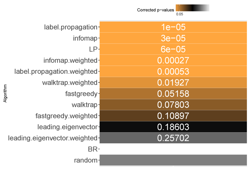
Figure 5.
Statistical evaluation of the method’s performance in terms of Jaccard similarity score. Gray, baseline; white, statistically identical to baseline; otherwise, the p-value of hypothesis that a method performs better than the baseline.
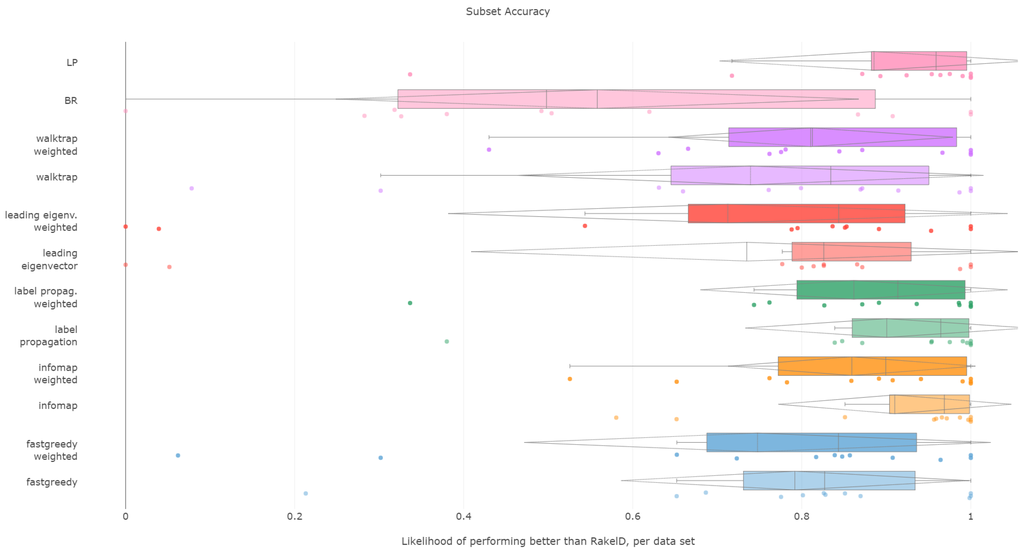
Figure 6.
Histogram of the methods’ likelihood of performing better than RAkELd in subset accuracy aggregated over datasets.
Table 3.
Likelihood of performing better than RAkELd in the subset accuracy of every method for each dataset.
Furthermore, unweighted infomap and label propagation are the most likely to yield results of higher subset accuracy than random label space divisions, both regarding the median (96%) and the mean (90% to 91%) likelihood. Label powerset follows with a 95.8% median and 89% mean. Weighted versions of infomap and label powerset are fourth and fifth with five to six percentage points less. We confirm RH2.
Concerning the resiliency of the advantage, only infomap versions proved to be better than RAkELd for more than half of the times: the unweighted version in 58% of cases, the weighted one in 52%. All other methods were below the 50% threshold in the worst case, with label powerset and label propagation likelihood of 33% for both variants. If one or two most wrong outliers were to be discarded, all methods are more than 50% likely to be better than random label space partitioning. We confirm RH3 and RH4.
We thus recommend using unweighted infomap as the data-driven alternative to RAkELd, as it is both significantly better than the random baseline, very likely to perform better than RAkELd and most resilient among the evaluated methods in the worst case. We confirm RH1, RH2, RH3 and RH4 for subset accuracy.
6.4. Jaccard Score
All methods apart from the weighted leading eigenvector modularity maximization approach were statistically significantly better than the average random baseline. Unweighted label propagation, label powerset and infomap were the highest ranked methods. We confirm RH1, with evidence provided in Figure 7 and Figure 8 and Table 4.
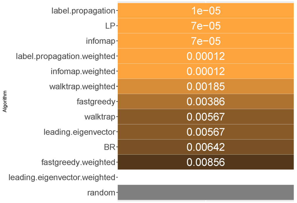
Figure 7.
Statistical evaluation of the method’s performance in terms of micro-averaged F1 score. Gray, baseline; white, statistically identical to baseline, otherwise; the p-value of the hypothesis that a method performs better than the baseline.
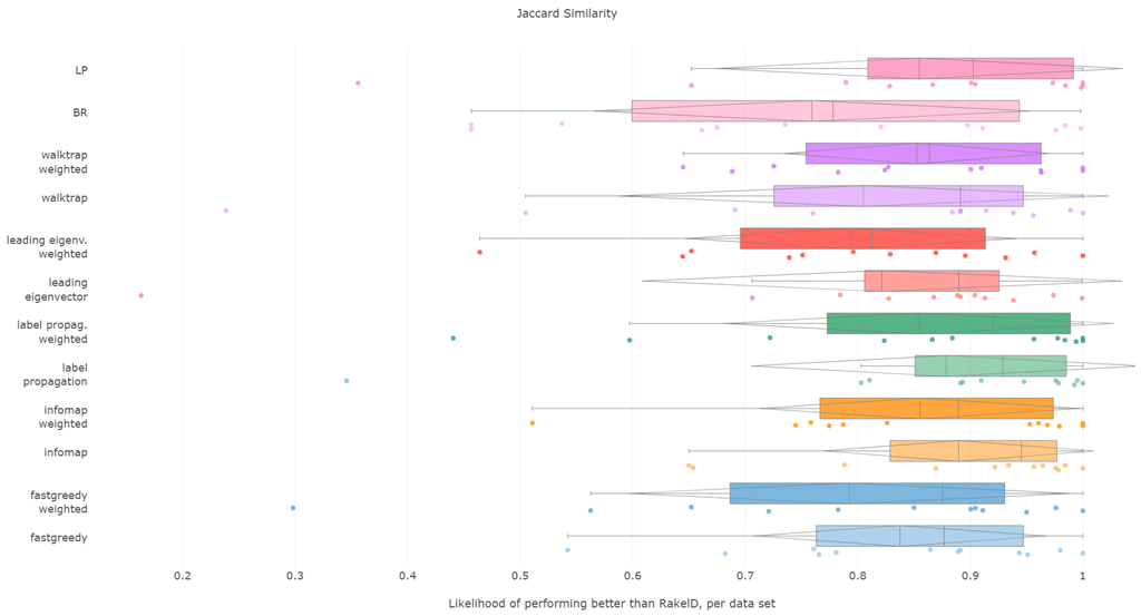
Figure 8.
Histogram of the methods’ likelihood of performing better than RAkELd in Jaccard similarity aggregated over datasets.
Table 4.
Likelihood of performing better than RAkELd in Jaccard similarity of every method for each dataset.
Jaccard score is similar to subset accuracy in rewarding exact label set matches. In effect, it is not surprising to see that unweighted infomap and label propagation are the most likely compared to RAkELd to yield a result of higher Jaccard score, both in terms of median (94.5% and 92.9%, respectively) and mean likelihoods (88.9% and 87.9%, resp.). Out of the two, infomap provides the most resilient advantage with a 65% probability of performing better than random approaches in the worst case. Label propagation is in the worst cases only 34% to 35% likely to be better than random space partitions.
We recommend using unweighted infomap approach over RAkELd when Jaccard similarity is of importance and confirm RH1, RH2, RH3 and RH4 for this measure.
6.5. Hamming Loss
Hamming loss is certainly a fascinating case in our experiments. As the measure is evaluated per each label separately, we can expect it to be the most stable over different label space partitions.
The first surprise comes with the Friedman–Iman–Davenport test result, where the test practically fails to find a difference in performance between random approaches and data-driven methods, yielding a p-value of . While the p-value is lower than , the difference cannot be taken as significant given the characteristics of the test. Lack of significance is confirmed by pairwise tests against random baseline (all hypotheses of difference are strongly rejected). We reject RH1, with evidence provided in Figure 9 and Table 5.
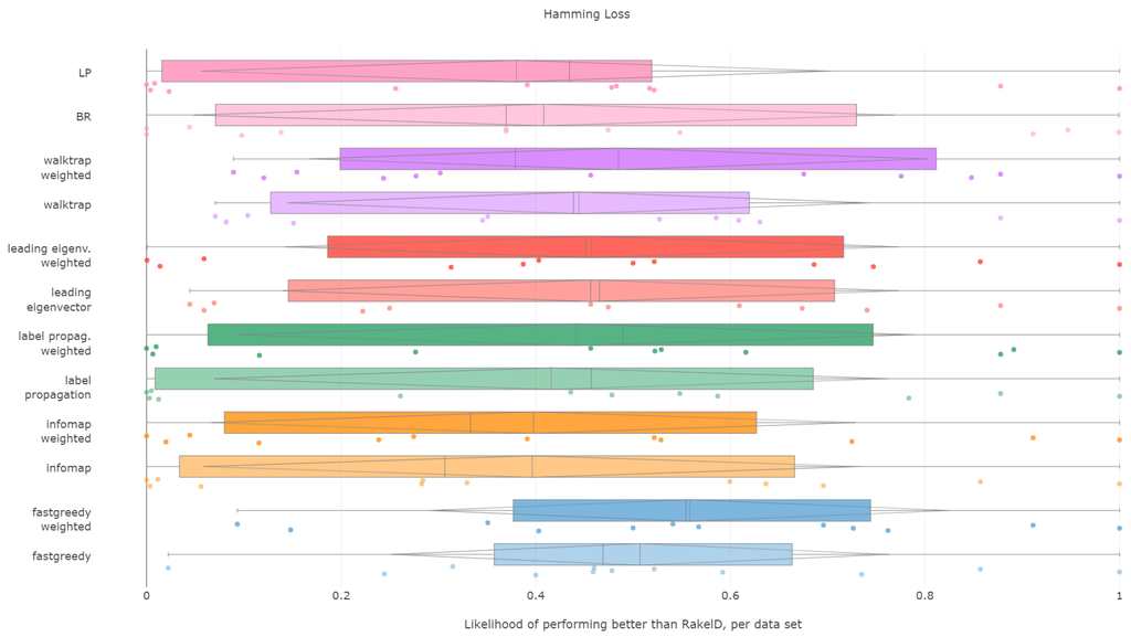
Figure 9.
Histogram of the methods’ likelihood of performing better than RAkELd in Hamming loss similarity aggregated over datasets.
Table 5.
Likelihood of performing better than RAkELd in Hamming loss of every method for each dataset.
Weighted fast greedy was the only approach to be more likely to yield a lower Hamming loss than RAkELd on average, both in median and mean (55%) likelihoods. The unweighted version was better than slightly over 50% more of the cases than RAkELd, with a median likelihood of 46%. Binary relevance and label powerset achieved likelihoods lower by close to 10 percentage points. We thus confirm RH2.
When it comes to worst-case observations binary relevance, label powerset and infomap in both variants were never better than RAkELd. The methods with the most resilient advantage in likelihood (9%) in the worst case were weighted versions of fast greedy and walktrap. We confirm RH3 and reject RH4.
We conclude that the fast greedy approach can be recommended over RAkELd, as even given such a large standard deviation (std) of likelihoods, it still yields lower Hamming loss than random label space divisions on more than half of the datasets. Yet, we reject RH1, RH2 and RH4 for Hamming loss. We confirm RH3, as a priori methods do not provide better performance than RAkELd in the worst case.
6.6. Efficiency
The efficiency comparison between the data-driven and random method for subspace division is of a special type. It is due to the fact that the data-driven approach requires a single run, whereas the random ones, a number of repetitions to get stable enough results. Thus, comparing the efficiency of both approaches, it must be based on the methods’ overall efficiency and not just the computation time of a single run/sampling.
The efficiency of label space partitioning approaches depends on the number of classifiers trained and the complexity of the partitioning procedure. In the case of the flat classification scheme, which we evaluate in this paper, the number of classifiers is equal to the number of subspaces into which the label space is partitioned. As all objects are classified by all sub-classifiers, the classification time is dependent on the single varying parameter: the label subspace size. RAkELd partitioning is performed in , as it is a procedure of randomly drawing a partition. The number of classifiers in the data-driven approach depends on the number of detected communities. Table 6 provides information about the number of detected communities in our experiments.
Table 6.
Number of communities (number of label subspaces) detected in training sets by each method per dataset.
That is why we evaluate the mean of the proportion between the running time of the data-driven approach to the time of running a single RAkELd, averaged per value of k. We compare this proportion to the average number of RAkELd runs required to match the average likelihood of data-driven approaches yielding better results of RAkELd per value of k, as only that number of RAkELd runs brings a high enough probability that enough samples were taken to yield comparable results. We call that point the efficiency threshold. If for example a data-driven method was better than 60% RAkELd samplings for a given k in a given measure and the total number of samplings for that value of k was 250, then the efficiency threshold for that value of k and that measure would be .
Efficiency figures presented in Appendix B (Figure B1, Figure B2, Figure B3, Figure B4 and Figure B5), are presented per method as log plots on the y axis of proportions averaged per k and thresholds per k per measure. We had to use log plots on the y axis due to the fact that the number of RAkELd runs equivalent to a single data-driven run was so greatly below the efficiency thresholds that the charts would not have been readable. Efficiency results do not vary much across methods; thus, we describe them collectively for all methods.
Points below baseline are cases when even a single iteration of RAkELd was slower than a single data-driven run. This happens when the number of classifiers in RAkELd is equal to 10, i.e., with of labels. The smaller the value of k becomes, the greater the efficiency of the data-driven methods becomes. As k increases, the number of classifiers trained by RAkELd decreases, and the single random run becomes faster. For most datasets, the data-driven approach running times become equivalent to six to eight RAkELd runs. The the worst case of data-driven running time reaching 15 RAkELd runs happens for large k on datasets genbase and medical. For these datasets, with a low level of label co-occurrence, the obtained co-occurrence graph is mostly disconnected, which yields many singletons, and that causes a large increase in the advantage of RAkELd over data-driven methods, as we never allow in the RAkELd scenario. What happens is that RAkELd trains few classifiers, and data-driven methods train more single-class classifiers representing singletons in the graph. We plan to improve this in the future by joining singletons into one subspace.
The slowest performance of data-driven methods was equivalent to 15 RAkELd runs. The average efficiency threshold of Hamming loss spanned between 50 and 70 runs of RAkELd, while other measures’ thresholds ranged between 80 and 110 runs. We thus note that RAkELd is far less efficient as a method than data-driven approaches, for every evaluated value of k.
We also note that before measuring efficiency per k, one needs to perform parameter estimation of the number of runs for RAkELd’ in our case, it would take at least ten runs of RAkELd, one for each value of of labels. One would usually want to repeat the procedure for each parameter value, at least a few times before selecting the value, as the variance in RAkELd performance is large. With data-driven methods, we gain a high likelihood of being better than RAkELd while running only one iteration.
We thus conclude that data-driven approaches are more efficient than RAkELd for every measure evaluated and for every value of k. We therefore accept RH5.
7. Conclusions
We have compared seven approaches as an alternative to random label space partition. RAkELd served as the random baseline for which we have drawn at most 250 distinct label space partitions for at most ten different values of the parameter k of label subset sizes. Out of the seven methods, five inferred the label space partitioning from training data in the datasets, while the two others were based on an a priori assumption on how to divide the label space. We evaluated these methods on 12 well-established benchmark datasets.
We conclude that in four of five measures, micro-/macro-averaged F1 score, subset accuracy and Jaccard similarity, all of our proposed methods were more likely to yield better scores than RAkELd apart from single outlying datasets; a data-driven approach was better than average random baseline with statistical significance at . The data-driven approach was also better than RAkELd in worst-case scenarios. Thus, hypotheses RH1, RH3 and RH4 have been successfully confirmed with these measures.
When it comes to Research Hypothesis 2 (RH2), we have confirmed that with micro-averaged F1, subset accuracy, Hamming loss and Jaccard similarity, the data-driven approaches have a higher likelihood of outperforming RAkELd than a priori methods do. The only exception to this is the case of macro-averaged F1, where binary relevance was most likely to beat random approaches, followed closely by a data-driven approach: weighted fast greedy.
Hamming loss forms a separate case for discussion, as this measures is most unrelated to label groups: it is calculated per label only. With this measure, most data-driven methods performed much worse than in other methods. Our study failed to observer a statistical difference between data-driven methods and the random baseline; thus, we reject hypothesis RH1. For best performing data-driven methods, the worst-case likelihood of yielding a lower Hamming loss than RAkELd was close to 10%, which is far from a resilient score; thus, we also reject RH4. We confirm RH2 and RH3, as there existed a data-driven approach that performed better than a priori approaches.
All in all, the statistical significance of a data-driven approach performing better than the averaged random baseline (RH1) has been confirmed for all measures, except Hamming loss. We have confirmed that the data-driven approach was more likely than binary relevance/label powerset to perform better than RAkELd (RH2) in all measures apart from the macro-averaged F1 score, where it followed the best binary relevance closely. Data-driven approaches were always more likely to outperform RAkELd in the worst case than binary relevance/label powerset, confirming RH3 for all measures. Finally, for all measures apart from Hamming loss, data-driven approaches were more likely to outperform RAkELd in the worst case, than otherwise. RH4 is thus confirmed for all measures, except Hamming loss.
In case of measures that are label-decomposable, the fast greedy community detection approach computed on a weighted label co-occurrence graph yielded the best results among data-driven perspectives and is the recommended choice for F1 measures and Hamming loss. When the measure is instance-decomposable and not label-decomposable, such as subset accuracy or Jaccard similarity, the infomap algorithm should be used on an unweighted label co-occurrence graph.
Data-driven methods also prove to be more time efficient than RAkELd. In case of small values of k, i.e., a large number of models trained by RAkELd, data-driven methods are more efficient than one iteration of RAkELd on most datasets, whereas the number of models decreases; the advantage of speed gained by RAkELd is not reflected in the likelihood of obtaining a result better than data-driven approaches provide in one run.
We conclude that community detection methods offer a viable alternative to both random and a priori assumption-based label space partitioning approaches. We summarize our findings in Table 7, answering the question in the title of how the data-driven approach to label space partitioning is likely to perform better than random choice.
Table 7.
The summary of the evaluated hypotheses and proposed recommendations of this paper.
Acknowledgments
The work was partially supported by the fellowship co-financed by the European Union within the European Social Fund; The European Commission under the 7th Framework Programme, Coordination and Support Action, Grant Agreement Number 316097 (ENGINE); the European Union’s Horizon 2020 research and innovation program under the Marie Skłodowska-Curie Grant Agreement No. 691152 (RENOIR); The National Science Centre research project 2014–2017 Decision No. DEC-2013/09/B/ST6/02317. This work was partially supported by the Faculty of Computer Science and Management, Wrocław University of Science and Technology statutory funds. Kristian Kersting acknowledges the support by the DFG Collaborative Research Center SFB 876 Project A6 “Resource Efficient Analysis of Graphs”. The authors wish to thank Łukasz Augustyniak for helping with proofreading the article.
Author Contributions
Piotr Szymański came up with the concept, conducted the experimental code and wrote most of the paper. Tomasz Kajdanowicz helped design the experiments, supported interpreting the results, supervised the work, wrote parts of the paper and corrected and proofread the paper. Kristian Kersting helped reorient the study towards the data-driven perspective, reorganizing and proofreading the paper. All authors have read and approved the final manuscript.
Conflicts of Interest
The authors declare no conflict of interest.
Appendix A. Result Tables
Table A1.
Number of random samplings from the universum of RAkELd label space partitions for cases different from 250 samples.
| Set Name | k | Number of Samplings |
|---|---|---|
| birds | 17 | 163 |
| emotions | 2 | 15 |
| 3 | 10 | |
| 4 | 15 | |
| 5 | 6 | |
| scene | 2 | 15 |
| 3 | 10 | |
| 4 | 15 | |
| 5 | 6 | |
| tmc2007-500 | 21 | 22 |
| yeast | 12 | 91 |
Table A2.
Likelihood of performing better than RAkELd in micro-averaged F1 score aggregated over datasets. Bold numbers signify the best likelihoods of a method performing better than RAkELd in the worst-case (Minimum) and average cases (Mean and Median).
| Minimum | Median | Mean | Std | |
|---|---|---|---|---|
| BR | 0.500000 | 0.885556 | 0.840028 | 0.152530 |
| LP | 0.438280 | 0.640237 | 0.704891 | 0.171726 |
| fast greedy | 0.565217 | 0.806757 | 0.820198 | 0.127463 |
| fast greedy-weighted | 0.673913 | 0.922643 | 0.863821 | 0.106477 |
| infomap | 0.478261 | 0.713565 | 0.720074 | 0.153453 |
| infomap-weighted | 0.433657 | 0.792426 | 0.748072 | 0.170349 |
| label_propagation | 0.364309 | 0.734100 | 0.717083 | 0.175682 |
| label_propagation-weighted | 0.478964 | 0.815100 | 0.750085 | 0.174347 |
| leading_eigenvector | 0.630606 | 0.783227 | 0.803901 | 0.116216 |
| leading_eigenvector-weighted | 0.630435 | 0.846506 | 0.834201 | 0.107420 |
| walktrap | 0.667500 | 0.742232 | 0.781920 | 0.102776 |
| walktrap-weighted | 0.695652 | 0.856861 | 0.852037 | 0.091232 |
Table A3.
Likelihood of performing better than RAkELd in macro-averaged F1 score aggregated over datasets. Bold numbers signify the best likelihoods of a method performing better than RAkELd in the worst-case (Minimum) and average cases (Mean and Median).
| Minimum | Median | Mean | Std | |
|---|---|---|---|---|
| BR | 0.500000 | 0.985683 | 0.919245 | 0.160273 |
| LP | 0.543478 | 0.829283 | 0.779482 | 0.163611 |
| fast greedy | 0.543478 | 0.883312 | 0.866478 | 0.139572 |
| fast greedy-weighted | 0.695652 | 0.969111 | 0.900483 | 0.116022 |
| infomap | 0.478261 | 0.820006 | 0.793086 | 0.147108 |
| infomap-weighted | 0.500000 | 0.889556 | 0.818476 | 0.164492 |
| label_propagation | 0.449376 | 0.801890 | 0.754205 | 0.182183 |
| label_propagation-weighted | 0.521739 | 0.855195 | 0.821663 | 0.148561 |
| leading_eigenvector | 0.695652 | 0.863565 | 0.851696 | 0.108860 |
| leading_eigenvector-weighted | 0.695652 | 0.889778 | 0.872119 | 0.118911 |
| walktrap | 0.695652 | 0.846889 | 0.844807 | 0.105977 |
| walktrap-weighted | 0.695652 | 0.894335 | 0.885253 | 0.095436 |
Table A4.
Likelihood of performing better than RAkELd in subset accuracy aggregated over datasets. Bold numbers signify the best likelihoods of a method performing better than RAkELd in the worst-case (Minimum) and average cases (Mean and Median).
| Minimum | Median | Mean | Std | |
|---|---|---|---|---|
| BR | 0.000000 | 0.498000 | 0.558057 | 0.323240 |
| LP | 0.336570 | 0.958889 | 0.885476 | 0.190809 |
| fast greedy | 0.213130 | 0.827043 | 0.791811 | 0.214756 |
| fast greedy-weighted | 0.061951 | 0.843413 | 0.747624 | 0.288200 |
| infomap | 0.580500 | 0.968667 | 0.910039 | 0.143954 |
| infomap-weighted | 0.525659 | 0.899430 | 0.859231 | 0.152637 |
| label_propagation | 0.380028 | 0.964444 | 0.900555 | 0.174854 |
| label_propagation-weighted | 0.336570 | 0.913652 | 0.861642 | 0.189690 |
| leading_eigenvector | 0.000000 | 0.826087 | 0.734935 | 0.340537 |
| leading_eigenvector-weighted | 0.000000 | 0.843778 | 0.712555 | 0.345277 |
| walktrap | 0.078132 | 0.834338 | 0.739359 | 0.288072 |
| walktrap-weighted | 0.429958 | 0.812667 | 0.810542 | 0.175723 |
Table A5.
Likelihood of performing better than RAkELd in Hamming loss aggregated over datasets. Bold numbers signify the best likelihoods of a method performing better than RAkELd in the worst-case (Minimum) and average cases (Mean and Median).
| Minimum | Median | Mean | Std | |
|---|---|---|---|---|
| BR | 0.000000 | 0.369565 | 0.408252 | 0.375954 |
| LP | 0.000000 | 0.434653 | 0.380021 | 0.338184 |
| fast greedy | 0.022222 | 0.469130 | 0.507034 | 0.266736 |
| fast greedy-weighted | 0.093333 | 0.554208 | 0.558218 | 0.280209 |
| infomap | 0.000000 | 0.306667 | 0.396299 | 0.352963 |
| infomap-weighted | 0.000000 | 0.332902 | 0.397576 | 0.345339 |
| label_propagation | 0.000000 | 0.457130 | 0.415966 | 0.361819 |
| label_propagation-weighted | 0.000000 | 0.489511 | 0.441813 | 0.363469 |
| leading_eigenvector | 0.044383 | 0.465511 | 0.456441 | 0.330251 |
| leading_eigenvector-weighted | 0.000444 | 0.451556 | 0.457361 | 0.328774 |
| walktrap | 0.070667 | 0.438943 | 0.444424 | 0.312845 |
| walktrap-weighted | 0.089333 | 0.379150 | 0.484974 | 0.331186 |
Table A6.
Likelihood of performing better than RAkELd in Jaccard similarity aggregated over datasets. Bold numbers signify the best likelihoods of a method performing better than RAkELd in the worst-case (Minimum) and average cases (Mean and Median).
| Minimum | Median | Mean | Std | |
|---|---|---|---|---|
| BR | 0.456522 | 0.778060 | 0.759178 | 0.202349 |
| LP | 0.355987 | 0.902632 | 0.854545 | 0.189086 |
| fast greedy | 0.542302 | 0.876667 | 0.837570 | 0.135707 |
| fast greedy-weighted | 0.298197 | 0.875222 | 0.792386 | 0.205646 |
| infomap | 0.650000 | 0.945261 | 0.889663 | 0.125510 |
| infomap-weighted | 0.510865 | 0.889488 | 0.855242 | 0.148578 |
| label_propagation | 0.345816 | 0.928789 | 0.878622 | 0.181165 |
| label_propagation-weighted | 0.440592 | 0.920261 | 0.853821 | 0.181186 |
| leading_eigenvector | 0.163199 | 0.889874 | 0.821436 | 0.222219 |
| leading_eigenvector-weighted | 0.464170 | 0.812444 | 0.794091 | 0.154102 |
| walktrap | 0.238558 | 0.891304 | 0.804866 | 0.227916 |
| walktrap-weighted | 0.644889 | 0.863722 | 0.852369 | 0.122837 |
Table A7.
The p-values of the assessment of the performance of the multi-label learning approaches compared against random baseline by the Iman–Davenport–Friedman multiple comparison, per measure.
| Iman–Davenport p-Value | |
|---|---|
| Subset Accuracy | 0.0000000004 |
| F1-macro | 0.0000000000 |
| F1-micro | 0.0000000177 |
| Hamming Loss | 0.0491215784 |
| Jaccard | 0.0000124790 |
Table A8.
The post-hoc pairwise comparison p-values of the assessment of the performance of the multi-label learning approaches compared against random baseline by the Iman–Davenport–Friedman test with Rom post hoc procedure, per measure. Bold numbers signify methods that perfomed statistically significantly better than RAkELd with a p-value .
| Accuracy | F1-macro | F1-micro | Hamming Loss | Jaccard | |
|---|---|---|---|---|---|
| BR | 0.3590121 | 0.0000003 | 0.0000500 | 1.0000000 | 0.0064229 |
| LP | 0.0000641 | 0.0280673 | 0.0205862 | 1.0000000 | 0.0000705 |
| fast greedy | 0.0515844 | 0.0000234 | 0.0000656 | 1.0000000 | 0.0038623 |
| fast greedy-weighted | 0.1089704 | 0.0000001 | 0.0000001 | 0.3472374 | 0.0085647 |
| infomap | 0.0000257 | 0.0484159 | 0.0205862 | 1.0000000 | 0.0000705 |
| infomap-weighted | 0.0002717 | 0.0010778 | 0.0024092 | 1.0000000 | 0.0001198 |
| label_propagation | 0.0000112 | 0.0484159 | 0.0205862 | 1.0000000 | 0.0000098 |
| label_propagation weighted | 0.0005315 | 0.0015858 | 0.0024092 | 1.0000000 | 0.0001196 |
| leading_eigenvector | 0.1860319 | 0.0001282 | 0.0002372 | 1.0000000 | 0.0056673 |
| leading_eigenvector-weighted | 0.2570154 | 0.0000274 | 0.0000653 | 1.0000000 | 0.0259068 |
| walktrap | 0.0780264 | 0.0000397 | 0.0004457 | 1.0000000 | 0.0056673 |
| walktrap-weighted | 0.0192676 | 0.0000239 | 0.0000040 | 1.0000000 | 0.0018482 |
Appendix B. Efficiency Figures
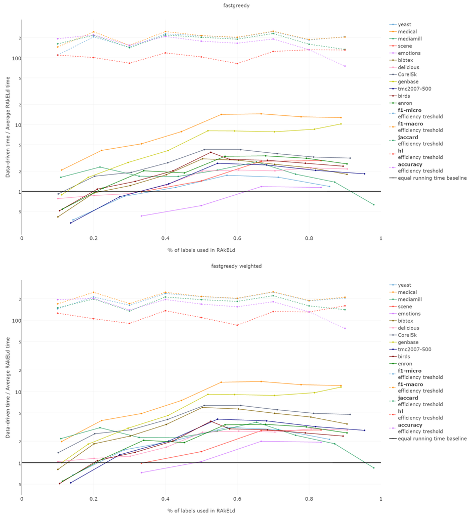
Figure B1.
Efficiency of fast greedy modularity maximization data-driven approach against RAkELd.
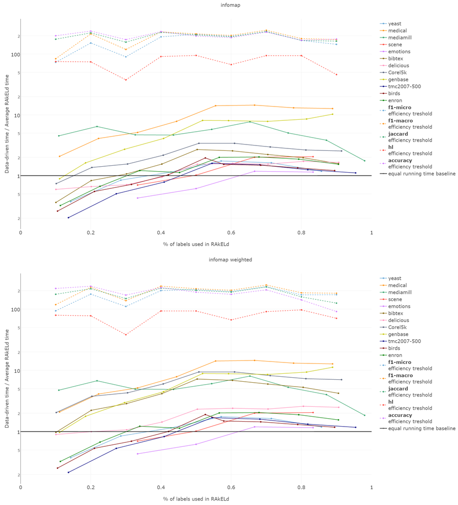
Figure B2.
Efficiency of the infomap greedy data-driven approach against RAkELd.
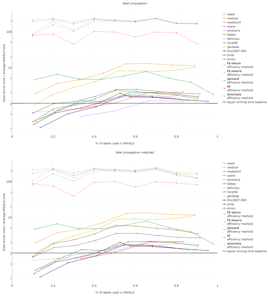
Figure B3.
Efficiency of the label propagation data-driven approach against RAkELd.
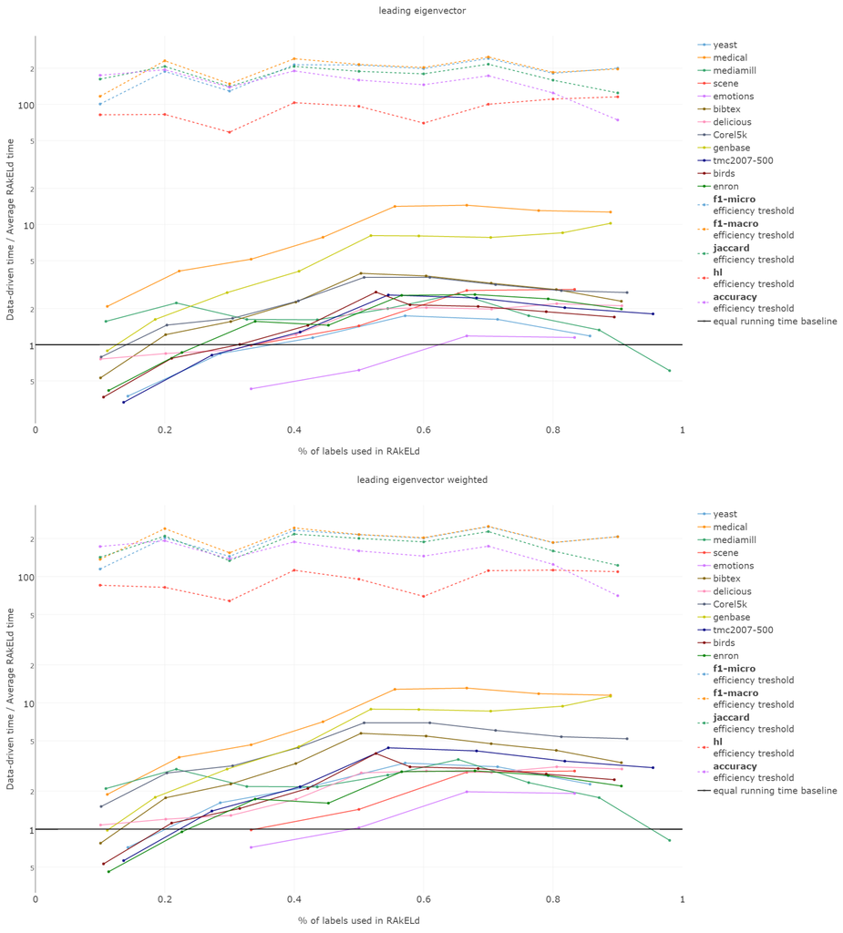
Figure B4.
Efficiency of the leading eigenvector modularity maximization data-driven approach against RAkELd.
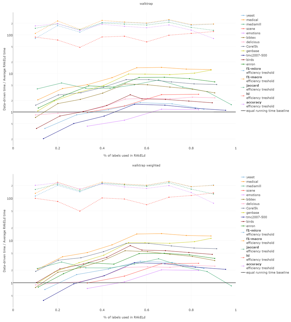
Figure B5.
Efficiency of the walktrap data-driven approach against RAkELd.
References
- Tsoumakas, G.; Katakis, I. Multi-label classification: An overview. Int. J. Data Warehous. Min. 2007, 3, 1–13. [Google Scholar] [CrossRef]
- Dembczyński, K.; Waegeman, W.; Cheng, W.; Hüllermeier, E. On label dependence and loss minimization in multi-label classification. Mach. Learn. 2012, 88, 5–45. [Google Scholar] [CrossRef]
- Tsoumakas, G.; Katakis, I.; Vlahavas, I. Random k-Labelsets for Multilabel Classification. IEEE Trans. Knowl. Data Eng. 2011, 23, 1079–1089. [Google Scholar] [CrossRef]
- Read, J.; Pfahringer, B.; Holmes, G.; Frank, E. Classifier chains for multi-label classification. Mach. Learn. 2011, 85, 333–359. [Google Scholar] [CrossRef]
- Dembczynski, K.; Cheng, W.; Hüllermeier, E. Bayes Optimal Multilabel Classification via Probabilistic Classifier Chains. In Proceedings of the 27th International Conference on Machine Learning (ICML-10), Haifa, Israel, 21–24 June 2010; pp. 279–286.
- Tsoumakas, G.; Katakis, I.; Vlahavas, I. Effective and efficient multilabel classification in domains with large number of labels. In Proceedings of the ECML/PKDD 2008 Workshop on Mining Multidimensional Data (MMD ‘08), Antwerp, Belgium, 19 September 2008; pp. 30–44.
- Madjarov, G.; Kocev, D.; Gjorgjevikj, D.; Džeroski, S. An extensive experimental comparison of methods for multi-label learning. Pattern Recognit. 2012, 45, 3084–3104. [Google Scholar] [CrossRef]
- Zhang, M.L.; Zhou, Z.H. A review on multi-label learning algorithms. IEEE Trans. Knowl. Data Eng. 2014, 26, 1819–1837. [Google Scholar] [CrossRef]
- Clauset, A.; Newman, M.E.J.; Moore, C. Finding community structure in very large networks. Phys. Rev. E 2004, 70, 066111. [Google Scholar] [CrossRef] [PubMed]
- Newman, M.E.J.; Girvan, M. Finding and evaluating community structure in networks. Phys. Rev. E 2004, 69, 026113. [Google Scholar] [CrossRef] [PubMed]
- Newman, M.E. Analysis of weighted networks. Phys. Rev. E 2004, 70, 056131. [Google Scholar] [CrossRef] [PubMed]
- Brandes, U.; Delling, D.; Gaertler, M.; Görke, R.; Hoefer, M.; Nikoloski, Z.; Wagner, D. On Modularity Clustering. IEEE Trans. Knowl. Data E 2008, 20, 172–188. [Google Scholar] [CrossRef]
- Newman, M.E.J. Finding community structure in networks using the eigenvectors of matrices. Phys. Rev. E 2006, 74, 036104. [Google Scholar] [CrossRef] [PubMed]
- Rosvall, M.; Axelsson, D.; Bergstrom, C.T. The map equation. Eur. Phys. J. Spec. Top. 2009, 178, 13–23. [Google Scholar] [CrossRef]
- Raghavan, U.N.; Albert, R.; Kumara, S. Near linear time algorithm to detect community structures in large-scale networks. Phys. Rev. E 2007, 76, 036106. [Google Scholar] [CrossRef] [PubMed]
- Pons, P.; Latapy, M. Computing communities in large networks using random walks (long version). 2005; arXiv:physics/0512106. [Google Scholar]
- MULAN. Available online: http://mulan.sourceforge.net/datasets-mlc.html (accessed on 21 July 2016).
- Katakis, I.; Tsoumakas, G.; Vlahavas, I. Multilabel text classification for automated tag suggestion. Available online: http://www.kde.cs.uni-kassel.de/ws/rsdc08/pdf/all_rsdc_v2.pdf#page=83 (accessed on 21 July 2016).
- Klimt, B.; Yang, Y. The enron corpus: A new dataset for email classification research. In Machine Learning: ECML 2004; Springer: Berlin/Heidelberg, Germany, 2004; pp. 217–226. [Google Scholar]
- UC Berkeley Enron Email Analysis. Available online: http://bailando.sims.berkeley.edu/enron_email.html (accessed on 21 July 2016).
- Computationalmedicine.org. Available online: http://www.computationalmedicine.org/challenge/ (accessed on 21 July 2016).
- Boutell, M.R.; Luo, J.; Shen, X.; Brown, C.M. Learning multi-label scene classification. Pattern Recognit. 2004, 37, 1757–1771. [Google Scholar] [CrossRef]
- Briggs, F.; Lakshminarayanan, B.; Neal, L.; Fern, X.Z.; Raich, R.; Hadley, S.J.K.; Hadley, A.S.; Betts, M.G. Acoustic classification of multiple simultaneous bird species: A multi-instance multi-label approach. J. Acoust. Soc. Am. 2012, 131, 4640–4650. [Google Scholar] [CrossRef] [PubMed]
- Briggs, F.; Huang, Y.; Raich, R.; Eftaxias, K.; Lei, Z.; Cukierski, W.; Hadley, S.; Hadley, A.; Betts, M.; Fern, X.; et al. The 9th annual MLSP competition: New methods for acoustic classification of multiple simultaneous bird species in a noisy environment. In Proceedings of the 2013 IEEE International Workshop on Machine Learning for Signal Processing (MLSP ‘13), Southampton, UK, 22–25 September 2013; pp. 1–8.
- Duygulu, P.; Barnard, K.; Freitas, J.F.G.D.; Forsyth, D.A. Object Recognition as Machine Translation: Learning a Lexicon for a Fixed Image Vocabulary. In Proceedings of the 7th European Conference on Computer Vision-Part IV (ECCV ‘02), Copenhagen, Denmark, 28–31 May 2012; pp. 97–112.
- Snoek, C.G.M.; Worring, M.; Gemert, J.C.V.; Geusebroek, J.M.; Smeulders, A.W.M. The challenge problem for automated detection of 101 semantic concepts in multimedia. In Proceedings of the ACM International Conference on Multimedia, Santa Barbara, CA, USA, 23–27 October 2006; pp. 421–430.
- MediaMill, Research on Visual Search. Available online: http://www.science.uva.nl/research/mediamill/challenge/ (accessed on 21 July 2016).
- Trohidis, K.; Tsoumakas, G.; Kalliris, G.; Vlahavas, I.P. Multi-Label Classification of Music into Emotions. In Proceedings of the Ninth International Conference on Music Information Retrieval (ISMIR 2008), Philadelphia, PA, USA, 14–18 September 2008; Volume 8, pp. 325–330.
- Elisseeff, A.; Weston, J. A Kernel Method for Multi-Labelled Classification. In Advances in Neural Information Processing Systems 14; MIT Press: Cambridge, MA, USA, 2001; pp. 681–687. [Google Scholar]
- Diplaris, S.; Tsoumakas, G.; Mitkas, P.A.; Vlahavas, I. Protein Classification with Multiple Algorithms. In Advances in Informatics; Springer: Berlin/Heidelberg, Germany, 2005; pp. 448–456. [Google Scholar]
- Derrac, J.; García, S.; Molina, D.; Herrera, F. A practical tutorial on the use of nonparametric statistical tests as a methodology for comparing evolutionary and swarm intelligence algorithms. Swarm Evol. Comput. 2011, 1, 3–18. [Google Scholar] [CrossRef]
- Demšar, J. Statistical Comparisons of Classifiers over Multiple Data Sets. J. Mach. Learn. Res. 2006, 7, 1–30. [Google Scholar]
- Scikit-Multilearn. Available online: http://scikit-multilearn.github.io/ (accessed on 21 July 2016).
- Pedregosa, F.; Varoquaux, G.; Gramfort, A.; Michel, V.; Thirion, B.; Grisel, O.; Blondel, M.; Prettenhofer, P.; Weiss, R.; Dubourg, V.; et al. Scikit-learn: Machine Learning in Python. J. Mach. Learn. Res. 2011, 12, 2825–2830. [Google Scholar]
- Tsoumakas, G.; Spyromitros-Xioufis, E.; Vilcek, J.; Vlahavas, I. Mulan: A Java Library for Multi-Label Learning. J. Mach. Learn. Res. 2011, 12, 2411–2414. [Google Scholar]
- Csardi, G.; Nepusz, T. The igraph software package for complex network research. Inter. J. Complex Syst. 2006, 1695, 1–9. [Google Scholar]
- Yang, Y. An Evaluation of Statistical Approaches to Text Categorization. Inf. Retr. 1999, 1, 69–90. [Google Scholar] [CrossRef]
© 2016 by the authors; licensee MDPI, Basel, Switzerland. This article is an open access article distributed under the terms and conditions of the Creative Commons Attribution (CC-BY) license (http://creativecommons.org/licenses/by/4.0/).