A Novel Image Encryption Scheme Using the Composite Discrete Chaotic System

Abstract

The composite discrete chaotic system (CDCS) is a complex chaotic system that combines two or more discrete chaotic systems. This system holds the chaotic characteristics of different chaotic systems in a random way and has more complex chaotic behaviors. In this paper, we aim to provide a novel image encryption algorithm based on a new two-dimensional (2D) CDCS. The proposed scheme consists of two parts: firstly, we propose a new 2D CDCS and analysis the chaotic behaviors, then, we introduce the bit-level permutation and pixel-level diffusion encryption architecture with the new CDCS to form the full proposed algorithm. Random values and the total information of the plain image are added into the diffusion procedure to enhance the security of the proposed algorithm. Both the theoretical analysis and simulations confirm the security of the proposed algorithm.

1. Introduction

With the rapid development of Internet and information technology, the secure transmission of image data becomes one of the most important problems. Due to some intrinsic features of image data, such as bulk data capacity, high redundancy and high correlation among adjacent pixels, traditional cryptosystems, for example, International Data Encryption Algorithm(IDEA), Data Encryption Standard (DES), and Advanced Encryption Standard (AES), are unsuitable for image data encryption [1,2,3]. It is well known that chaos theory has many unique characteristics, such as ergodicity, pseudo randomness, sensitivity to initial conditions and control parameters [4], and these characteristics meet the requirements of diffusion and mixing in the sense of cryptography. Hence, chaotic system has become a good choice for image encryption. Since the first chaos-based image encryption scheme was proposed by Fridrich [1], many chaos-based image encryption schemes can be found in recent literatures. Because low dimensional chaotic maps have the advantages of simplicity and efficiency, researchers in [5] realized an encryption scheme for color images permutated by using zigzag path scrambling with a spatiotemporal chaotic system. A RGB image encryption based on total image characteristics and modified Logistic map are presented in [6]. In [7], the authors presented a novel image encryption algorithm based on Henon map and compound spatiotemporal chaos with s superiority key sensitivity, plaintext sensitivity, and execution efficiency. Zhou et al. provided an image encryption algorithm with a simple structure and integrates the Logistic, Sine and Tent maps into one single system in [8]. However, these algorithms have some limitations, such as small key size and weak security. Recently, the purpose of using high dimensional chaotic maps and hyper chaotic systems is to enlarge the key space of the algorithms and resist brute force attack. For instance, a fast image encryption algorithm with a new two-dimensional Sine iterative chaotic map with infinite collapse (ICMIC) modulation map where the confusion and diffusion processes are combined for one stage with hyper chaotic behavior was introduced in [9]. Hua et al. proposed two new 2-dimensional (2D) Sine-Logistic modulation maps which were derived from the Logistic and Sine maps with wider chaotic range, better ergodicity, hyper chaotic property and relatively low implementation cost in [10,11]. In [12], Mollaeefar et al. provided a novel method for color image encryption based on high level chaotic maps Cosinus-Arcsinus and Sinus-Power Logistic map, which have better chaotic behavior against other available chaotic maps. Hyper-chaos has two or more Lyapunov exponents, and it indicates that the dynamics of this system is expanded in more than one direction instability [13,14,15,16]. Wang et al. in [13] proposed an effective image encryption algorithm based on genetic recombination and hyper-chaotic system. A new lossless encryption algorithm for color images based on a 6D hyper chaotic system and the 2D discrete wavelet transform in both the frequency domain and the spatial domain with key streams depend on the hyper chaotic system and the plain image is shown in [14]. Wu et al. in [15] introduced a novel color image cryptosystem based on synchronization of two different 6D hyper chaotic systems. Zhu et al. in [16] permutated the plain image twice by a discrete 2D hyper-chaos system to obtain good permutated effect. Moreover, many researchers suggested that composite chaotic system could be utilized to enhance the complexity and security level of the algorithm, because composite chaotic system may possess better randomness and complex chaotic character so that the cryptosystem can obtain higher security. Tong et al. in [17] adopted the Feistel network and constructed a Cubic function in the encryption algorithm and its key space was larger which was more efficiency and low resource depletion. A novel color image encryption algorithm was proposed based on the complex Chen and complex Lorenz systems, where One pixel in a channel may appear in any position and any channel in [18]. In [19,20,21], the authors provided several image encryption schemes with compound chaotic system by exploiting two 1D chaotic functions which switch randomly. All these references show the compound chaotic system has a better performance in speed, complexity, and security and can solve the problem that unable to resist short periods and low precision of low dimensional chaotic function by perturbation.

Besides the classic substitution-diffusion architecture, there are also other proposed chaos-based image encryption algorithms with their own structures. For example, the basic unit of an image can also be represented as bit (for example, a pixel value 54 can be represented as “00110110”). Some bit-level image encryption algorithms can be found in [22,23,24,25], which can play a permutation and diffusion effect simultaneously by a bit-level permutation. Zhu et al. in [22] proposed an image cryptosystem employing the 2D Arnold map for bit-level permutation, and this cryptosystem can obtain diffusion effect and save some encryption time. A new 3D bit matrix permutation algorithm was proposed where an image was considered as a natural three dimensional bit matrix (width, height, and bit length) in [23]. Fu et al. in [24] studied a symmetric chaos-based image cipher with a 3D cat map-based spatial bit-level permutation strategy where the diffusion effect of the new method was superior as the bits were shuffled among different bit-planes rather than within the same bit-plane. Zhu et al. in [25] arranged the positions of each bit by the generalized Arnold map in both row and column directions in a random way to get permutation and diffusion effect, then used affine cipher to obtain better diffusion effect to avoid the similarity existing in the bit-level permutation stage. Moreover, in [26], a novel image encryption scheme was proposed based on reversible cellular automata combining chaos. In [27,28], image encryption schemes based on DNA sequence operations rule and some improved chaotic systems were proposed, and an image encryption algorithm based on wave function and chaotic system was given in [29] where keystream was dependent on both the plain image and the secret key. However, some chaos-based image encryptions had been broken [30,31,32,33,34]. According to the Kerckhoff’s principle, the security level of cryptographic keys decides the security level of the cipher algorithms. To improve the security level of the chaos-based image encryption scheme, researchers have also attempted to generate good keystream providing cryptographic keys used in image encryption schemes. As an illustration, Seyedzadeh et al. in [35] designed a fast color image encryption algorithm based on a coupled two-dimensional piecewise chaotic map by a 256-bit external secret key as session keys. A 256-bit long hash value that depended on the three plain images was used to generate three random sequences to design a triple image encryption algorithm in [36].

In this paper, we aim to provide a novel image encryption method based on a composite discrete chaotic system with high chaotic behaviors, and a single permutation and double-diffusion operation are realized with scanning the plain image one time, which will lead to good encryption effect. Moreover, random values and the total information of the plain image are added into the diffusion procedure. As a result, the obtained cipher images are totally different even using the same secret key to encrypt a plain image several times. The rest of this paper is organized as follows.

In Section 2, we design a new composite discrete chaotic system (CDCS) that combines different chaotic systems in a random way, which can enhance the chaotic behaviors of the single chaotic system. In Section 3, we employ CDCS to perform the bit-level permutation and pixel-level diffusion operation to form the full proposed algorithm, and obtain a better diffusion effect. In Section 4, we analyze the security of the proposed scheme and evaluate its performance with several comparable algorithms through key size analysis, histogram analysis, chi-square test, correlation analysis, information entropy analysis, local Shannon entropy analysis, key sensitivity analysis, chosen/known plaintext attacks analysis, differential attack analysis, speed performance analysis, and the robustness of the proposed algorithm in noise and data loss. Finally, we summarize the main results in Section 5.

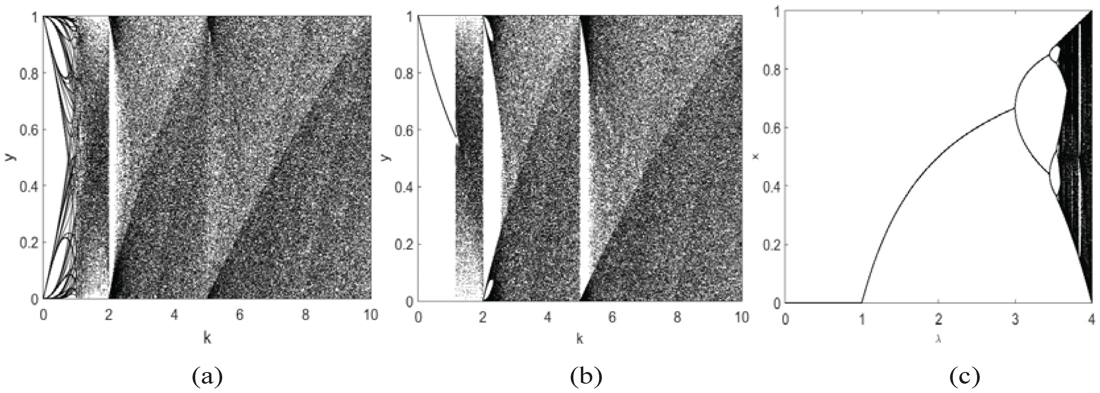
2. Composite Discrete Chaotic System

2.1. Two-Dimensional Composite Discrete Chaotic System

CDCS is a specific chaotic system combining two or more discrete chaotic systems. The merit of the new CDCS is that it can choose different chaotic system in the iteration procedure in a random way. The definition of the CDCS is given below:

Definition 1. 

Let $x_i=f_q(x_{i-1}),q=0,1,\cdots ,m-1,i=1,2,\cdots$ be m different discrete chaotic systems. For a random composite sequence $S=\{s_1,s_2,\cdots \}\in {\{0,1,\cdots ,m-1\}}^{\infty }$, we call the following functions an m-dimensional CDCS

$$x_i=f_{s_i}(x_{i-1}),i=0,1,\cdots ,m-1.$$

(1)

We denote this system as $(f_0,f_1,\cdots ,f_{m-1},S)$.

Definition 1 implies that the chaotic behavior of CDCS relies on the random composite chaotic sequence S and every discrete chaotic system in CDCS. Generally, the chaotic characteristics of CDCS is more complicated than that in every single chaotic system. Note that, if $m=1$ or $s_i$ is a constant, CDCS degenerates to an ordinary single chaotic system.

Theorem 2. 

Let $f_q(x),q=0,1,\cdots ,m-1$, be m functions in Definition 1. If $|f_q^{\prime }(x)|>1$, then for any random composite chaotic sequence S, the m-dimensional CDCS is chaotic.

Proof of Theorem 2. 

Let $S=\{s_1,s_2,\cdots \}\in {\{0,1,\cdots ,m-1\}}^{\infty }$ be a random composite chaotic sequence, $\left\{x_n\right\}$ is iterated by Equation (1) with initial value $x_0$, with a simple computation. The Lyapunov exponent of the CDCS is

$$\lambda =\underset{n\to \infty }{lim}\frac{1}{n}log|\prod f_{s_n}^{\prime }(x_n)|>0.$$

(2)

We know that positive Lyapunov exponent means chaos. Thus, the m-dimensional CDCS is chaotic. This completes the proof. ☐

According to Theorem 2, we design a 2-dimensional CDCS by the following Equations (3) and (4):

$$f_0(x)=\left\{\begin{array}{c}\sqrt{1-kx}0<x<\frac{1}{k},\hfill \\ 1-\sqrt{kx-1}\frac{1}{k}\le x\le 1,\hfill \end{array}\right.$$

(3)

$$f_1(x)=\left\{\begin{array}{c}1-\sqrt{1-kx}0<x<\frac{1}{k},\hfill \\ \sqrt{kx-1}\frac{1}{k}\le x\le 1,\hfill \end{array}\right.$$

(4)

where $k\ge 2,k\in \mathbf{N}$.

Note that

$$f_0^{\prime }(x)=\left\{\begin{array}{c}-\frac{k}{2\sqrt{1-kx}}0<x<\frac{1}{k},\hfill \\ -\frac{k}{2\sqrt{kx-1}}\frac{1}{k}\le x\le 1,\hfill \end{array}\right.$$

(5)

$$f_1^{\prime }(x)=\left\{\begin{array}{c}\frac{k}{2\sqrt{1-kx}}0<x<\frac{1}{k},\hfill \\ \frac{k}{2\sqrt{kx-1}}\frac{1}{k}\le x\le 1,\hfill \end{array}\right.$$

(6)

and, $|f_i^{\prime }(x)|>1,i=0,1$. Thus, the new CDCS is chaotic by Theorem 2.

2.2. Sensitivity Analysis of the Initial Values and Control Parameters in CDCS

A good chaotic system must be sensitive to initial values and control parameters, respectively. First, we generate a chaotic random sequence X by Chebyshev map $x_{n+1}=F(x_n)=cos(\beta \times arccos(x_n))$, $n=0,1,\cdots ,x_n\in [-1,1].$ with initial value $\beta =\pi ,x_0=0.436879342$, then, we quantify it by $y=\lceil x\ast {10}^9\rceil (mod2)$, and obtain the composite random sequence S.

Now, we consider the initial value sensitivity of the proposed CDCS, with the help of the composite random sequence S, we set the initial value $x_0=0.65382364$, $0.65382365$ from the Chebyshev chaotic sequence X and $k=2$ in Equations (3) and (4), and iterate it 2010 times and get two chaotic sequences, respectively. The first 2000 iterated random real numbers are discarded to avoid the harmful effect of CDCS, and the last 10 iterated random real numbers are shown in

Table 1. Chaotic sequences generated by CDCS with different initial value.

Chaotic Sequence	x0 = 0.65382364	x0 = 0.65382365
$y_{2001}$	0.6916087935	0.5510774642
$y_{2002}$	0.6190457067	0.3196168464
$y_{2003}$	0.4879461173	0.3993617501
$y_{2004}$	0.8447332446	0.5513615043
$y_{2005}$	0.8303411884	0.3205043035
$y_{2006}$	0.8128237059	0.4008410954
$y_{2007}$	0.7909787683	0.5546711225
$y_{2008}$	0.7250674640	0.3306693894
$y_{2009}$	0.6974535701	0.4180539361
$y_{2010}$	0.6709209552	0.595164073

. From Table 1, we know that the two chaotic sequences are very different though the initial values are just a trivial difference (${10}^{-8}$). So, CDCS is very sensitive to initial value.

Notice that the different control parameter k in Equations (3) and (4) means different CDCS. In order to see the sensitivity of the control parameter k in CDCS, we diffuse the plain image (lena) with the following steps:

Step 1: 

Get 6 different CDCS by setting $k=2,3,4,5,6,7$, respectively. Then, we obtain 6 chaotic sequences with the initial value $x_0=0.65382364$ by Equations (3) and (4), respectively. If the output $|y_i|$ is larger than 1, then we let $y_i=\frac{\sqrt{k-1}-y_i}{\sqrt{k-1}}$ in Equation (3) and $y_i=\frac{\sqrt{k-1}-1+y_i}{\sqrt{k-1}-1}$ in Equation (4), and if the output $y_i<0$, then $y_i=\left|y_i\right|$. Next, we turn them into 6 binary sequence by $y=\lceil x\ast {10}^9\rceil mod2$.

Step 2: 

Extend the plain gray image matrix to an 1-dimensional integer sequence, and transform the integer sequence into a binary sequence.

Step 3: 

Do exclusive OR for the binary sequence with the 6 chaotic binary sequences, respectively, then get 6 diffused binary sequences

Step 4: 

Transform the 6 diffused binary sequences into 6 integer sequences, and reshape them into 6 diffused images. The diffusion effect is shown in Figure 1. From Figure 1, we know that each CDCS can get good diffuse effect.

We also list the differences of the six diffused images in

Table 2. The differences among diffused images by CDCS with different k.

Control Parameter	k = 2	k = 3	k = 4	k = 5	k = 6	k = 7
k = 2	0	0.99607849	0.99603271	0.99586487	0.99604797	0.99598694
k = 3	0.99607849	0	0.99621582	0.99627686	0.99639893	0.9962616
k = 4	0.99603271	0.99621582	0	0.99629211	0.99645996	0.9962616
k = 5	0.99586487	0.99627686	0.99629211	0	0.99615479	0.99568176
k = 6	0.99604797	0.99639893	0.99645996	0.99615479	0	0.99591064
k = 7	0.99598694	0.9962616	0.9962616	0.99568176	0.99591064	0

.

The computation results show that the diffuse effect is very sensitive to the control parameter k in CDCS even with the same initial value. Therefore, CDCS is very sensitive to the initial values and control parameters.

2.3. Trajectory

For a chaotic system, the trajectory means the movement of the outputs, Figure 2 shows the trajectories of different chaotic maps: the CDCS of Equations (3) and (4); the single chaotic map Equation (3), and the Logistic map. Their parameters are set to the values that ensure both the maps to have excellent chaotic behaviors. The initial value are set to the same. From Figure 2, the trajectory of the CDCS distributes in much larger regions in the whole plane than that of the comparable chaotic maps. It means the CDCS is more random and has better ergodicity properties.

2.4. Gottwald and Melbourne Test

In 2004, Georg Gottwald and Ian Melbourne introduced a new test for chaos [37]. The input is any time series from a discrete map, a differential equation etc. The output is a real number in [0,1], which in theory is either 0, for non-chaotic data, or 1, for chaotic data. In practice, the result is close to 0 means non-chaotic, and close to 1 means chaotic, we use different parameters paris $(x_0,k)$ to generate different CDCS sequences, and do the Gottwald and Melbourne test in

Table 3. The Gottwald and Melbourne test.

Initial Value x0	Control Parameters k	Test Results
0.12345678	k = 2	0.99823000
0.12345679	k = 2	0.99839183
0.12345677	k = 2	0.99790976
0.12345676	k = 2	0.99798716
0.21345678	k= 3	0.99782871
0.21345678	k = 4	0.99831404
0.21345678	k = 5	0.99842179
0.21345678	k = 6	0.99854142
0.321345678	k = 7	0.99735072

, and we conclude that the CDCS has good chaotic behaviors.

3. The Proposed Scheme

Base on the discussion in Section 2, we are now ready to describe the proposed image encryption algorithm. The diagram of the proposed algorithm is shown in Figure 3.

3.1. Secret Key Generation

The secret keys of the proposed scheme actually are consisted of the following parts: (1) the initial value $x_0^{\prime }$ and control parameter $k_0^{\prime }$ of Chebyshev map for generating composite sequence S; (2) the 8 initial values $x_1^{\prime },x_2^{\prime },\cdots ,x_8^{\prime }$ and 8 control parameters $k_1^{\prime },k_2^{\prime },\cdots ,k_8^{\prime }$ of CDCS used in permutation stage; (3) the initial values and control parameters $x_9^{\prime }$, $x_{10}^{\prime }$, $k_9^{\prime }$ and $k_{10}^{\prime }$ of CDCS for generating random sequences $ran{d}_1$ and $ran{d}_2$ in the diffusion stage. We represent them $K=(A,B)$, where $A=(x_0^{\prime },x_1^{\prime },x_2^{\prime },\cdots ,x_{10}^{\prime })$, $B=(k_0^{\prime },k_1^{\prime },k_2^{\prime },\cdots ,k_{10}^{\prime })$. In order to satisfy the security requirement, we set a random key with the length of 505 bits to generate the secret key $K=(A,B)$ used in the proposed algorithm of the proposed algorithm, the detailed procedure is shown in the Algorithm 1:

Algorithm 1. The generation of the secret key

Input: Random key K with length of 505 bits

Output: Secret key $(A,B)$ used in the proposed algorithm.

1: $i=1$;

2: for $j=0:1:10$;

3:   $x_j=({\sum }_{t=0}^{24}K[i+t]\times 2^t)/2^{25}$;

4:   $i=i+25$;

5: end for

6: for $j=0:1:10$;

7:   $k_j=({\sum }_{t=0}^{9}K[i+t]\times 2^t)/2^{10}$;

8:   $i=i+10$;

9: end for

10: for $j=0:1:10$;

11:   $s_j=({\sum }_{t=0}^{9}K[i+t]\times 2^t)/2^{10}$;

12:   $i=i+10$;

13: end for

14:   $a=({\sum }_{t=0}^{9}K[496+t]\times 2^t)/2^{10}$;

15:   $k_0^{\prime }=(k_0\times mod1)+3$;

16: for $j=0:1:10$

17:   $x_j^{\prime }=(x_j+a\times s_j)mod1$

18: end for

19: for $j=1:1:10$

20:   $k_j^{\prime }=(round((k_j+a\times s_j)mod1\times {10}^9)mod32$;

21: end for

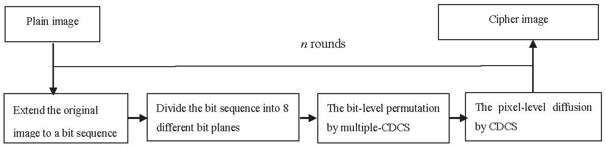
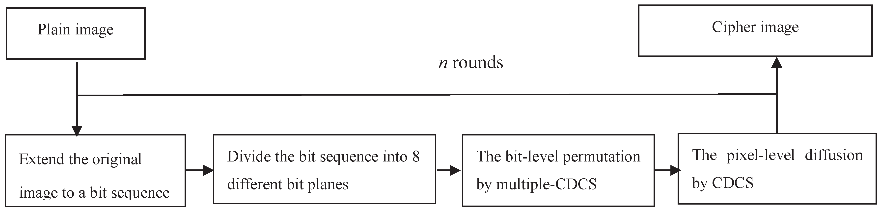
3.2. Encryption Process

There are two parts in the encryption algorithm: one is a bit-level permutation stage, and the other is a pixel-level diffusion procedure. Permutation in an image encryption architecture can be classified into pixel-level permutation and bit-level permutation. In this paper, we denote a plain image by a $3\times 3$ matrix M to show the bit-level permutation effect:

$$M=\left[\begin{array}{ccc}{p}_1& p_2& p_3\\ p_4& p_5& p_6\\ p_7& p_8& p_9\end{array}\right].$$

(7)

If we do a pixel-level permutation, only the position of the pixel is changed and the value of the pixel remains unchanged. However, if we consider the bit-level permutation, we extend M to a column vector ${(p_1,p_2,\cdots ,p_9)}^T$, and change each pixel $p_i$ into a 8-bits binary sequence $\{p_{i_1},p_{i_2},\cdots ,p_{i_8}\},$ $i=1,2,\cdots ,9$, and get a new 2-dimensional binary matrix $M_1$:

$$M_1=\left[\begin{array}{cccccccc}{p}_{11}& p_{12}& p_{13}& p_{14}& p_{15}& p_{16}& p_{17}& p_{18}\\ p_{21}& p_{22}& p_{23}& p_{24}& p_{25}& p_{26}& p_{27}& p_{28}\\ p_{31}& p_{32}& p_{33}& p_{34}& p_{35}& p_{36}& p_{37}& p_{38}\\ p_{41}& p_{42}& p_{43}& p_{44}& p_{45}& p_{46}& p_{47}& p_{48}\\ p_{51}& p_{52}& p_{53}& p_{54}& p_{55}& p_{56}& p_{57}& p_{58}\\ p_{61}& p_{62}& p_{63}& p_{64}& p_{65}& p_{66}& p_{67}& p_{68}\\ p_{71}& p_{72}& p_{73}& p_{74}& p_{75}& p_{76}& p_{77}& p_{78}\\ p_{81}& p_{82}& p_{83}& p_{84}& p_{85}& p_{86}& p_{87}& p_{88}\\ p_{91}& p_{92}& p_{93}& p_{94}& p_{95}& p_{96}& p_{97}& p_{98}\end{array}\right].$$

(8)

Then, we extend $M_1$ to a binary sequence and do the bit-level permutation. Moreover, we reshape the shuffled binary sequence to form the permutated binary matrix:

$$M_2=\left[\begin{array}{cccccccc}{p}_{94}& p_{61}& p_{57}& p_{58}& p_{93}& p_{43}& p_{53}& p_{62}\\ p_{95}& p_{66}& p_{12}& p_{44}& p_{54}& p_{63}& p_{96}& p_{67}\\ p_{72}& p_{32}& p_{87}& p_{18}& p_{13}& p_{45}& p_{84}& p_{51}\\ p_{55}& p_{64}& p_{97}& p_{68}& p_{73}& p_{33}& p_{75}& p_{35}\\ p_{25}& p_{88}& p_{21}& p_{14}& p_{77}& p_{37}& p_{46}& p_{27}\\ p_{85}& p_{24}& p_{83}& p_{17}& p_{11}& p_{52}& p_{92}& p_{56}\\ p_{42}& p_{65}& p_{73}& p_{98}& p_{71}& p_{31}& p_{86}& p_{48}\\ p_{74}& p_{34}& p_{76}& p_{26}& p_{23}& p_{82}& p_{16}& p_{91}\\ p_{41}& p_{28}& p_{47}& p_{22}& p_{81}& p_{15}& p_{38}& p_{78}\end{array}\right].$$

(9)

From $M_2$, we can see that both the positions of the bits and the value of the pixels are changed. Hence, a significant diffusion effect occurs in the bit-level permutation procedure. Finally, we turn every row of $M_2$ into an integer according to the normal order and get nine integers $p_1^{\prime },p_2^{\prime },\cdots ,p_9^{\prime }$, then we reshape them into the permutated image as follows:

$$\left[\begin{array}{ccc}{p}_1^{\prime }& p_2^{\prime }& p_3^{\prime }\\ p_4^{\prime }& p_5^{\prime }& p_6^{\prime }\\ p_7^{\prime }& p_8^{\prime }& p_9^{\prime }\end{array}\right].$$

(10)

3.2.1. Bit-Level Permutation Stage

In this subsection, we denote a plain image with size $h\ast w$ as ${(a_{ij})}_{h\times w}$, and we use multiple-CDCS mentioned in Equations (3) and (4) to do the bit-level permutation operation. The detailed process is stated as follows:

Step 1: 

Extend the plain image gray value matrix ${(a_{ij})}_{h\times w}$ to a binary sequence: $E=\{E_1,E_2,\cdots ,E_{h\ast 8w}\}$. Then, turn E into 8 different bit planes: $B_1,B_2,\cdots ,B_8$ by the following rules: $B_1=\left\{E_i\right|i\equiv 1mod8,i=1,2,\cdots ,h\ast 8w\}$, $B_2=\left\{E_i\right|i\equiv 2mod8,i=1,2,\cdots ,h\ast 8w\}$, $B_3=\left\{E_i\right|i\equiv 3mod8,i=1,2,\cdots ,h\ast 8w\}$, $B_4=\left\{E_i\right|i\equiv 4mod8,i=1,2,\cdots ,h\ast 8w\}$, $B_5=\left\{E_i\right|i\equiv 5mod8,i=1,2,\cdots ,h\ast 8w\}$, $B_6=\left\{E_i\right|i\equiv 6mod8,i=1,2,\cdots ,h\ast 8w\}$, $B_7=\left\{E_i\right|i\equiv 7mod8,i=1,2,\cdots ,h\ast 8w\}$, $B_8=\left\{E_i\right|i\equiv 0mod8,i=1,2,\cdots ,h\ast 8w\}$.

Step 2: 

Get 8 chaotic sequences of size $w\ast h$ by Equations (3) and (4) with 8 pairs parameters ($x_0$, k), and denote them as $F_i=\{F_{i1},F_{i2},\cdots ,F_{iw\ast h}\},i=1,\cdots ,8$. If the output $|y_i|$ is larger than 1, we let $y_i=\frac{\sqrt{k-1}-y_i}{\sqrt{k-1}}$ in Equation (3) and $y_i=\frac{\sqrt{k-1}-1+y_i}{\sqrt{k-1}-1}$ in Equation (4), and if the output $y_i<0$, then $y_i=\left|y_i\right|$. Then, sort $F_i$ in ascending order and get 8 index order sequences $I_i=\{I_{i1},I_{i2},\cdots ,I_{ih\ast w}\},i=1,2,\cdots ,8$.

Step 3: 

Permutate the binary sequence $B_i$ by $I_i$ in the following way to get a shuffled binary sequence $T_i=\left\{T_{ij}\right|j=1,2,\cdots ,h\ast w\}$:

$$\begin{array}{c}\hfill T_{ij}=B_{I_{ij}},i=1,\cdots ,8,j=1,\cdots ,h\ast w\end{array}$$

Step 4: 

Rearrange the 8 permutated binary sequences $T_i,i=1,2,\cdots ,8$ into the permutated sequence J with size $h\ast 8w$ in the following way:

$$J=\{T_{11},T_{21},\cdots ,T_{81},T_{12},T_{22},\cdots ,T_{82},\cdots ,T_{1h\ast w},T_{2h\ast w},\cdots ,T_{8h\ast w}\}$$

Step 5: 

Divide the intermediate binary sequence J into $h\ast w$ blocks: $K_1=\{J_1,J_2,\cdots ,J_8\}$, $K_2=\{J_9,J_{10},\cdots ,J_{16}\}$, ⋯, $K_{(h\ast w)}=\{J_{h\ast 8w-7},J_{h\ast 8w-6},\cdots ,J_{h\ast 8w}\}$, then change each block into an integer, and get the permutated integer sequence $Int=\{Int(1),Int(2),\cdots ,Int(h\ast w)\}$, and reshape to the permutated image.

The permutated image of plain image lena and the histogram distribution image are shown in Figure 4c–d. From Figure 4c–d, we note that the bit-level permutation process hides the information and changes the statistical characters of the plain image. Unfortunately, the image has some similarity in the histogram distribution and it is not absolutely uniform, thus, the attacker will find some useful information with this similarity and break this scheme. Therefore, we do the pixel-level diffusion operation to overcome this defect.

3.2.2. Pixel-Level Diffusion Stage

In the bit-level permutation phase, we obtain a shuffled integer sequence $Int=\{Int(1),Int(2),\cdots ,Int(h\ast w)\}$, now we do the pixel-level diffusion operation in the following steps:

Step 1: 

Obtain 2 CDCS chaotic sequences by Equations (3) and (4), and quantify with $y=\lceil x\ast {10}^9\rceil mod256$, then name $ran{d}_1$ and $ran{d}_2$, respectively.

Step 2: 

For each $Int(k)\in Int,k=1,2,\cdots ,h\ast w$, do the following operations:

$$\{\begin{array}{l}te{m}_2=Int(k)\oplus te{m}_1\oplus ran{d}_2(k)\\ C(k)=(ran{d}_1(te{m}_0)+te{m}_2),mod256\\ te{m}_0=k;te{m}_1=C(k)\end{array}$$

(11)

In Equation (11), the initial value $te{m}_0=\lceil cos(\pi arccos(x_0+\sum a_{ij}/{10}^9))\ast {10}^9\rceil mod256$, $te{m}_1=\lceil cos(\pi arccos(x_1+\sum a_{ij}/{10}^9))\ast {10}^9\rceil mod256$, where $x_0$ and $x_1$ are random value, $a_{ij}$ is the i-th row and the j-th pixel of the plain image, respectively. $C(k)$ is the final encrypted value of the k-th pixel value.

Step 3: 

Reshape the encrypted integer sequence C back to the 2-dimensional gray value matrix of size $h\ast w$ to form the finally encrypted image.

3.3. Decryption Process

Note that the decryption procedure is just the inverse of the encryption procedure, hence, we introduce it briefly as follows:

3.3.1. Pixel-Level Diffusion Decryption Stage

Step 1: 

For the encrypted image, turn it into an integer sequence: $C=\{C(1),C(2),\cdots ,C(h\ast w)\}$.

Step 2: 

Obtain 2 CDCS chaotic sequences again by Equations (3) and (4) with the same parameters used in the encryption procedure, respectively. Then they are quantified by $y=\lceil x\ast {10}^9\rceil mod256$ and named $ran{d}_1^{\prime }$, $ran{d}_2^{\prime }$, respectively.

Step 3: 

Let the initial value $te{m}_0^{\prime }=h\ast w-1,te{m}_1^{\prime }=C(h\ast w-1)$. For each $C(k)\in C,k=h\ast w,h\ast (w-1),\cdots ,2$, do the following operations to get the permutated sequence $In{t}^{\prime }$:

$$\{\begin{array}{l}te{m}_2^{\prime }=(C(k)-ran{d}_1^{\prime }(te{m}_0^{\prime })),(mod256),\\ In{t}^{\prime }(k)=te{m}_2^{\prime }\oplus te{m}_1^{\prime }\oplus ran{d}_2^{\prime }(k-1),\\ te{m}_0^{\prime }=k-1;te{m}_1^{\prime }=C(k-1).\end{array}$$

(12)

Note that when $k=1$, in order to get $In{t}^{\prime }(1)$, in Equation (12), we let $te{m}_0^{\prime }=\lceil cos(\pi arccos(x_0+\sum a_{ij}/{10}^9)\ast {10}^9\rceil mod256$, $te{m}_1^{\prime }=\lceil cos(\pi arccos(x_1+\sum a_{ij}/{10}^9)\ast {10}^9\rceil mod256$, where $x_0,x_1$ are the same used in the encryption procedure.

3.3.2. Bit-Level Permutation Decryption Stage

With the decryption of pixel-level diffusion, we get the decrypted sequence $In{t}^{\prime }$. Now, we depict the bit-level permutation decryption.

Step 1: 

Extend the decrypted sequence $In{t}^{\prime }$ to a binary sequence $G=\{g_1,g_2,\cdots ,g_{h\ast 8w}\}$, where $h\ast w$ is the length of $In{t}^{\prime }$, respectively. Then, turn binary sequence G into 8 different bit planes $T_1,T_2,\cdots ,T_8$ by the following rules: $T_1=\left\{g_i\right|i\equiv 1mod8,i=1,2,\cdots ,h\ast 8w\}$, $T_2=\left\{g_i\right|i\equiv 2mod8,i=1,2,\cdots ,h\ast 8w\}$, $T_3=\left\{g_i\right|i\equiv 3mod8,i=1,2,\cdots ,h\ast 8w\}$, $T_4=\left\{g_i\right|i\equiv 4mod8,i=1,2,\cdots ,h\ast 8w\}$, $T_5=\left\{g_i\right|i\equiv 5mod8,i=1,2,\cdots ,h\ast 8w\}$, $T_6=\left\{g_i\right|i\equiv 6mod8,i=1,2,\cdots ,h\ast 8w\}$, $T_7=\left\{g_i\right|i\equiv 7mod8,i=1,2,\cdots ,h\ast 8w\}$, $T_8=\left\{g_i\right|i\equiv 0mod8,i=1,2,\cdots ,h\ast 8w\}$.

Step 2: 

Get the 8 chaotic sequences of size $w\times h$ again by Equations (3) and (4) with the 8 pairs same parameters ($x_0$, k) used in the encryption procedure, and denote them as $H_i=\{H_{i1},H_{i2},\cdots ,H_{iw\ast h}\},i=1,\cdots ,8$. If the output $|y_i|$ is larger than 1, we let $y_i=\frac{\sqrt{k-1}-y_i}{\sqrt{k-1}}$ in Equation (3) and $y_i=\frac{\sqrt{k-1}-1+y_i}{\sqrt{k-1}-1}$ in Equation (4), and if the output $y_i<0$, then $y_i=\left|y_i\right|$. Then, sort $H_i$ in ascending order and get 8 index order sequences $I_i^{\prime }=\{I_{i1}^{\prime },I_{i2}^{\prime },\cdots ,I_{ih\ast w}^{\prime }\},i=1,2,\cdots ,8$.

Step 3: 

Permutate the binary sequence $T_i$ by $I_i^{\prime }$, in the following way to obtain the original binary sequence $B_i^{\prime }$:

$$\begin{array}{c}\hfill B_{I_{ij}^{\prime }}^{\prime }=T_{ij}=,i=1,\cdots ,8,j=1,\cdots ,h\ast w\end{array}$$

Step 4: 

Rearrange the 8 permutated binary sequences $B_1^{\prime },\cdots ,B_8^{\prime }$ into the permutated sequence P of size $h\ast 8w$ in the following way: $Q=\{B_1^{\prime }(1),B_2^{\prime }(1),\cdots ,B_8^{\prime }(1)$, $B_1^{\prime }(2),B_2^{\prime }(2),\cdots ,B_8^{\prime }(2),\cdots ,$ $B_1^{\prime }(h\ast w),B_2^{\prime }(h\ast w),\cdots ,B_8^{\prime }(h\ast w)\}$.

Step 5: 

Divide the intermediate binary sequence Q into $(h\ast w)$ blocks: $Y_1=\{B_1^{\prime },B_2^{\prime },\cdots ,B_8^{\prime }\}$, $Y_2=\{B_9^{\prime },B_{10}^{\prime },\cdots ,B_{16}^{\prime }\}$, ⋯, $Y_{h\ast w}=\{B_{h\ast 8w-7}^{\prime },B_{h\ast 8w-6}^{\prime },\cdots ,B_{h\ast 8w}\}$, then turn each block into an integer, and get the decrypted integer sequence $P=\{P(1),P(2),\cdots ,P(h\ast w)\}$.

Step 6: 

Reshape the decrypted integer sequence P back to the 2-dimensional gray value matrix of size $h\ast w$ to get the finally decrypted image.

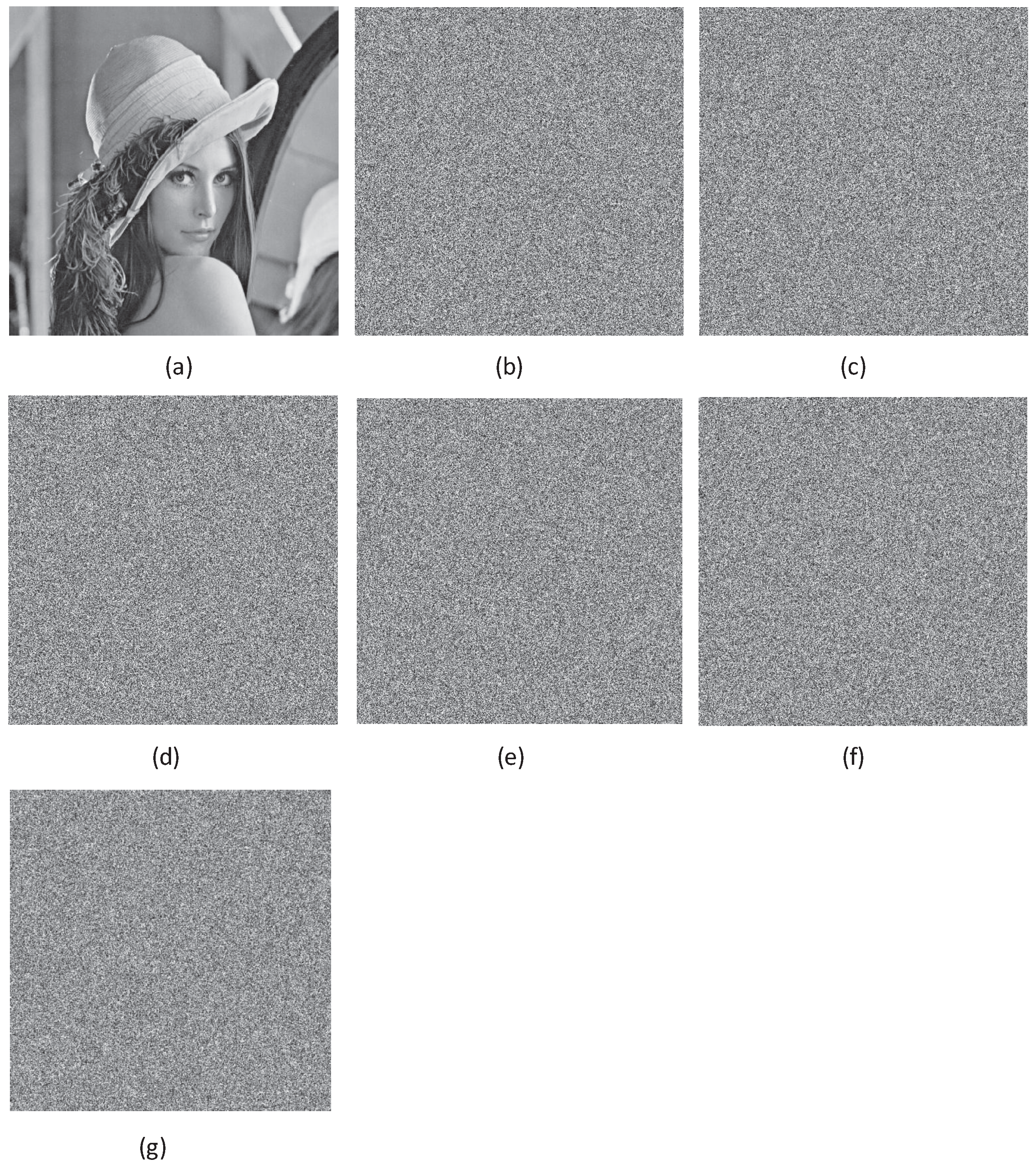
4. Simulation Results and Security Analyses

In this section, we use test images from the USC-SIPI “Miscellaneous” image [38]. Simulation results performance analyses for the proposed scheme and four comparable algorithms are provided. They include key size analysis, histogram analysis, chi-square test, correlation analysis, information entropy analysis, local shannon entropy analysis, key sensitivity analysis, chosen/known plaintext attacks analysis, differential attack analysis, speed performance analysis, and the robustness of the proposed algorithm in noise and data loss. All the simulations are performed on a personal computer (Hewlett-Packard, Shenyang, China) with an Intel Core 3.1 HZ CPU, 4G memory, and 450 GB hard disk with a Windows 7 Ultimate operating system, and the compile platform is Matlab (Version 2013a).

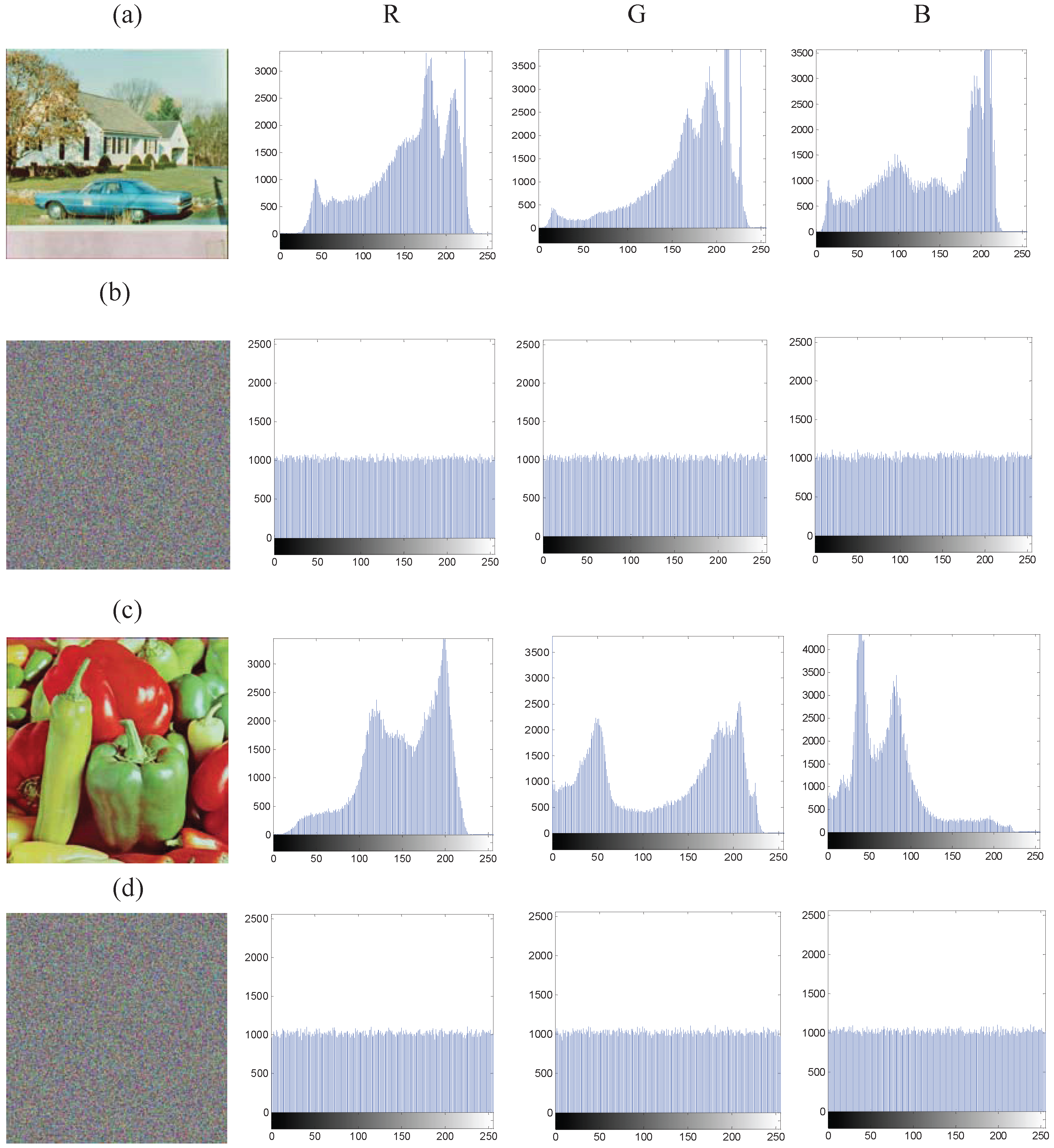
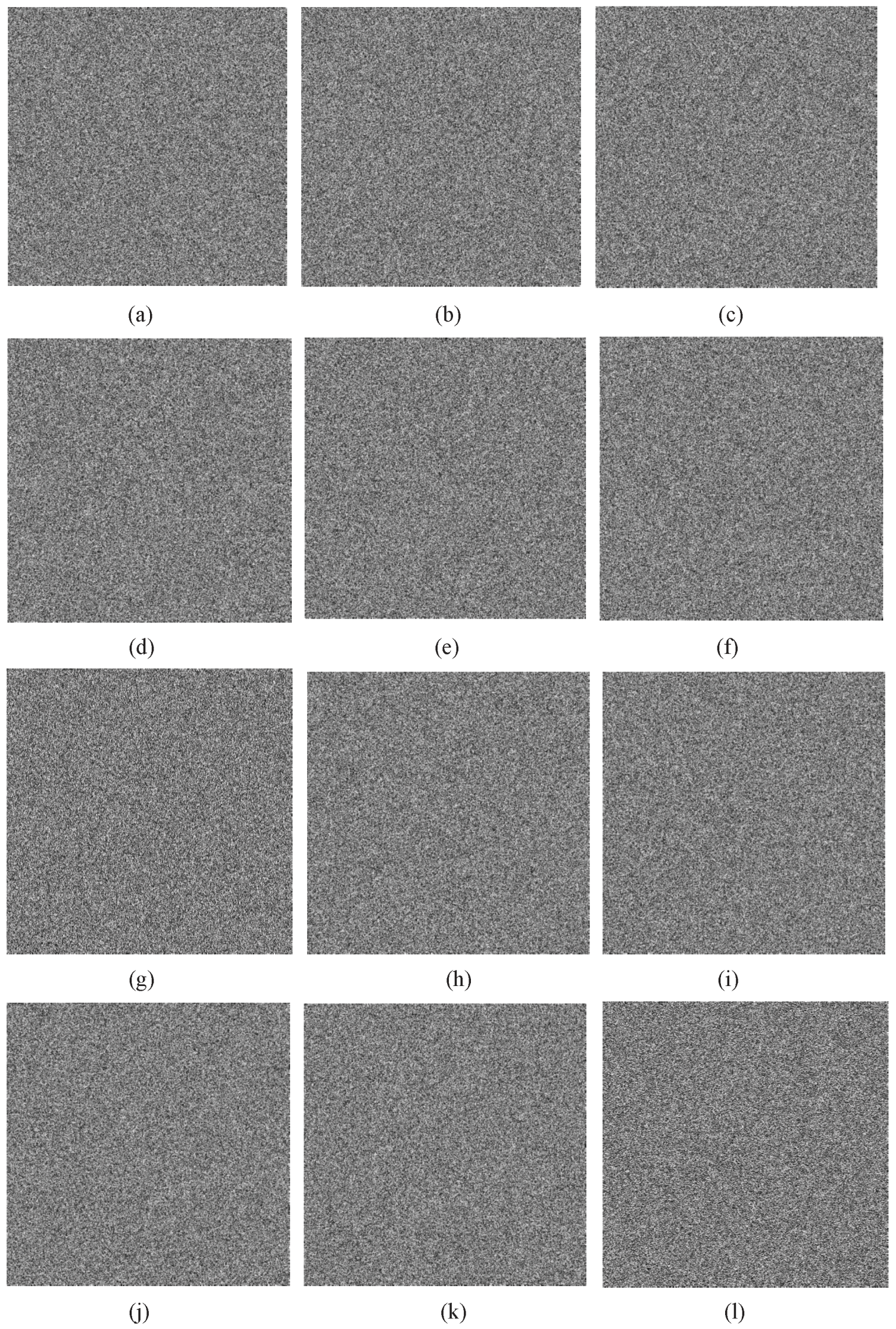
4.1. Gray and Color Image Encryption

Because of the spectrum of digital images around the world, the proposed algorithm must encrypt any image with similar results in security and performance. In this subsection, we use some images (include gray and color image) with different histogram for encryption and security analysis to verify the algorithm capabilities. Figure 4a,b,e,f shows the gray plain image and its histogram, the encrypted image and the corresponding histogram; Figure 5a–d shows two color plain images and the cipher images with their corresponding histograms. As a result, the gray cipher image, the RGB components of cipher images, and the uniform histograms verify the proposed algorithm’s ability to encrypt any gray and color image.

4.2. Key Size Analysis

According to the Kerckhoff’s principle, the security level of an image encryption scheme relies on the randomness of the cryptographic keys. As we know, to provide an encryption algorithm with high security, the key space should be more than $2^{100}$ to make brute force attack ineffective. In this subsection, we use 505 bits random hexadecimal digits as secret key, and generate the key used in the proposed algorithm in Section 3.1. From the generation procedure, with a simple computation, we can conclude that the proposed algorithm has large enough key size to resist the brute force attack.

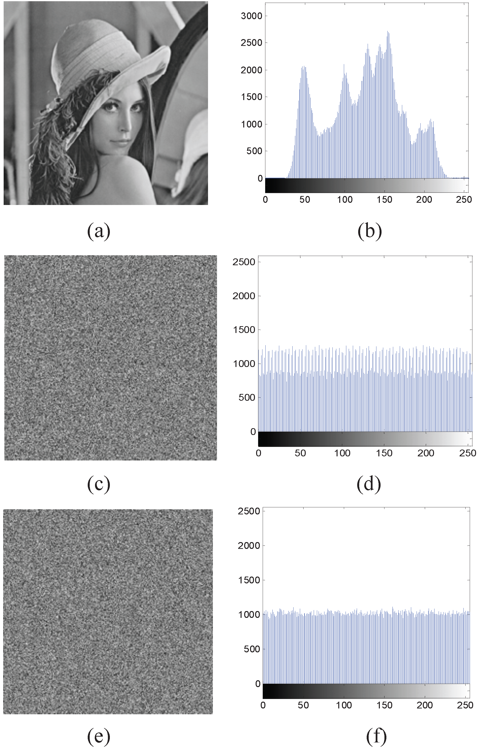
4.3. The Chi-Square Test Analysis of Cipher Image

The histogram distribution contains the information distribution of pixel values in an image. An ideal encrypted image should have a uniform histogram distribution to prevent the opponent from extracting any useful information from the fluctuating histogram. Figure 4a,b depicts the original lena image and its histogram, Figure 4e,f shows the encrypted image and corresponding histogram distribution obtained by the proposed scheme. Figure 5a–d shows 2 color plain images and the cipher image with their corresponding histograms. It is clear that the gray value and RGB component histogram of the encrypted images are fairly uniform and significantly different from that of the plain images. Hence, it does not provide any clue to employ statistical attack on the proposed algorithm.

Except for the cipher image histogram distribution analysis graphically, in order to show the uniform of the cipher image more precise, we also use the chi-square test to show that the cipher image is a uniform histogram distribution. The chi-square test produces a p-value which is a real number in [0,1]. If the p-value of a test image is greater than a significant level α, the test image passes the test successfully. In our experiment, we compute the p-value of some test images from the USC-SIPI “Miscellaneous” image dataset, and set α = 0.05, the results are listed in

Table 4. Chi-square test analysis (α = 0.05).

Image Name	p-value
5.2.08	0.257198003
5.2.09	0.22534446
5.2.10	0.220229861
7.1.01	0.200104753
7.1.02	0.115958523
7.1.03	0.478716242
7.1.04	0.477272383
7.1.05	0.536532281
7.1.06	0.681580846
7.1.07	0.492913738
7.1.08	0.919338576
7.1.09	0.101262279
boat.512	0.631836356
elaine	0.52057636
lena	0.224053673
goldhill	0.883876476
peppers	0.13530398
baboon	0.763747416
house(R)	0.099225363
house(G)	0.412077954
house(B)	0.285299456

. From Table 4, all the test images pass the chi-square test, so, the cipher image is a uniform histogram distribution.

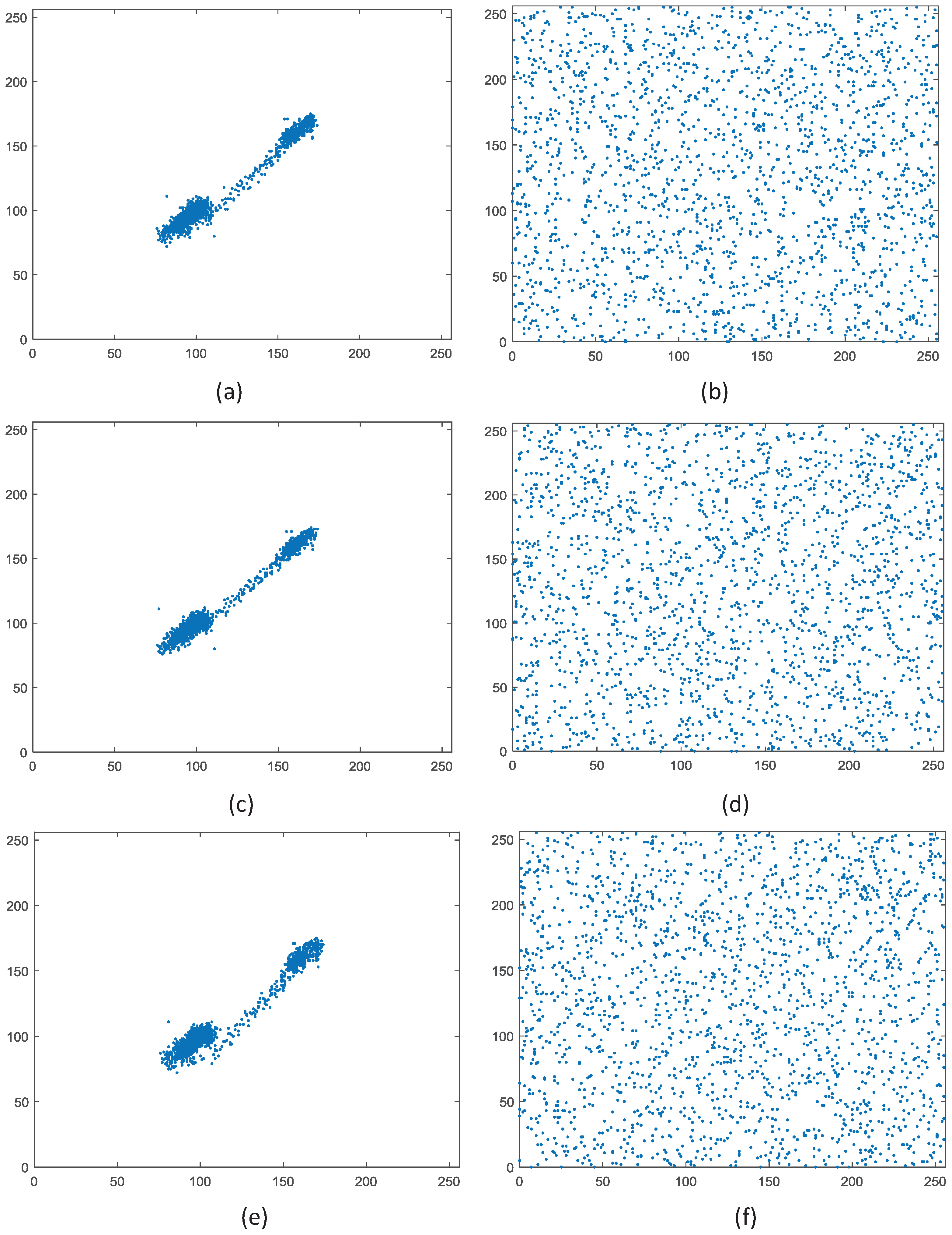
4.4. Correlation Analysis

In this subsection, correlation analysis is performed on the plain image and encrypted image to examine the encryption effect of our scheme. It is well known that the correlation between plain image adjacent pixels is high and should be reduced in the encrypted image for a good encryption scheme. Thus, we randomly select 2000 pairs of pixel values among two horizontally, two vertically, and two diagonally adjacent pixels in the plain image and cipher image, respectively, then we calculate the correlation coefficient $r_{xy}$ in

Table 5. Correlation coefficients analysis. (Numbers in bold face means the crresoponding encryption scheme has the smallest correlation coefficients.)

Test Image	Direction	Plain Image	Proposed Scheme	Ref. [16]	Ref. [22]	Ref. [8]	Ref. [25]
	horizontal	0.98727175	0.00911870	−0.01598859	0.00921633	−0.03444986	0.0255741
lena	vertical	0.99060282	−0.02799349	−0.00928994	0.00438226	0.0162397	−0.0060722
	diagonal	0.98232025	−0.008005781	0.00955705	0.00984828	0.05472108	0.03712793
	horizontal	0.98359562	0.00984443	−0.01681935	0.02161067	0.04823954	0.00106722
goldhill	vertical	0.97498297	0.01843329	0.03527012	0.03929575	−0.01953583	0.01852442
	diagonal	0.96849169	0.002687612	0.006798479	0.02047153	−0.01473057	0.01321081
	horizontal	0.98486792	0.06072394	0.0237943	0.02161067	−0.00350778	−0.0115003
peppers	vertical	0.97916019	−0.00116499	−0.011170982	−0.037837	−0.021423	−0.00237434
	diagonal	0.97515696	−0.00571419	0.00664635	0.02047153	0.02345089	−0.00098435
	horizontal	0.74954747	−0.03856932	−0.02999071	0.0161014	0.00289877	−0.00547718
house(R)	vertical	0.80262072	0.002023	−0.0154941	−0.04053886	0.018131106	−0.01215746
	diagonal	0.60609133	0.00207905	−0.01487206	−0.00227398	0.018180302	−0.01803246
	horizontal	0.76294284	0.00181239	−0.0161565	0.0485065	−0.00423018	−0.03230305
house(G)	vertical	0.86429319	−0.01279169	−0.00183728	0.01576013	0.00157326	0.0002708
	diagonal	0.66868095	0.00241394	0.00156149	−0.03474189	-0.003761	−0.00867577
	horizontal	0.90852712	−0.00921239	0.02068469	0.015610986	−0.04302791	0.02820804
house(B)	vertical	0.9477393	0.0034053	−0.02170484	−0.00567228	0.0137757	0.0107359
	diagonal	0.86744223	−0.0217718	−0.0075945	0.01271975	0.00921989	0.03581673

by the following formula:

$$r_{xy}=\frac{|E((x-E(x))(y-E(y)))|}{\sqrt{D(x)D(y)}}$$

(13)

where $E(x)$ and $D(x)$ are the expectation and variance of variable x, respectively.

From Table 5, we see that, in the 9 correlation coefficients of the 3 gray test images, 5 correlation coefficients are smaller than that in the comparable algorithms, and 5 correlation coefficients of the color image are smaller than the comparable algorithm. Moreover, the correlation coefficients in the 3 directions of the encrypted image are close to 0, thus, the high correlation in the plain image is significantly reduced by the proposed scheme. To show this feature graphically, the correlation distributions of adjacent pixels of plain image lena and encrypted image in the 3 directions can be seen in Figure 6a–f. The results show that the dots of plain image lena are focused on the diagonal, while those of the encrypted image are scattered uniformly over the entire plane. In summary, all of data and graphs show that the high correlations in plain gray and color image are significantly reduced in the encrypted image by the proposed scheme.

4.5. Information Entropy Analysis

Global information entropy is the measure on the uncertainty of an information source. Obviously, the ideal information entropy value for a 8 bits true randomly message is 8. Here, we use $H(X)$ to represent the information entropy of the information source $X=(x_0,x_1,\cdots ,x_{L-1})$ by the following Equation (14):

$$H(X)=-\sum _{i=0}^{L-1}p(x_i)lo{g}_{2}p(x_i).$$

(14)

The information entropy of some different test images are listed in

Table 6. Information entropy analysis.

Test Image	Plain Image	The Proposed Scheme	Ref. [16]	Ref. [22]	Ref. [8]	Ref. [25]
5.2.08	7.201008	7.9992989	7.9970096	7.9993075	7.999206	7.9993742
5.2.09	6.9939942	7.9992833	7.9968423	7.9992492	7.9991342	7.9992579
5.2.10	5.7055602	7.9992883	7.9969656	7.9993485	7.9992213	7.9993323
7.1.01	6.0274148	7.9993239	7.9972729	7.9993146	7.9991445	7.9993389
7.1.02	4.0044994	7.9993947	7.9931779	7.999289	7.9989956	7.9993285
7.1.03	5.49574	7.9992167	7.997577	7.9993951	7.9991431	7.9993135
7.1.04	6.1074181	7.9991862	7.9970146	7.9993017	7.999126	7.9993481
7.1.05	6.5631956	7.9992767	7.9969023	7.9993046	7.9991403	7.9993864
7.1.06	6.6952834	7.999398	7.9975578	7.999246	7.9992993	7.9992284
7.1.07	5.9915988	7.9992502	7.997237	7.9992476	7.9989706	7.9992728
7.1.08	5.053448	7.9992442	7.9967758	7.9993288	7.9989898	7.9991881
7.1.09	6.1898137	7.99938	7.9972559	7.9991956	7.9991552	7.9992166
boat.512	7.1913702	7.9993893	7.997026	7.99931	7.9991832	7.9993511
lena	7.4455676	7.9993283	7.9973605	7.9993589	7.999155	7.9992604
goldhill	7.4777796	7.9993354	7.9974798	7.9992933	7.9992657	7.999319
baboon	7.3735278	7.9992275	7.9970364	7.9993183	7.9991787	7.9993072
peppers	7.5714776	7.9992535	7.9974015	7.9991921	7.9992645	7.9992152
elaine	7.4664262	7.9993301	7.9972385	7.9993498	7.9991789	7.9992656
house(R)	7.415627	7.9992942	7.9970608	7.999344	7.9992396	7.9992674
house(G)	7.2294792	7.9993214	7.9974495	7.9992617	7.9991642	7.9993073
house(B)	7.4353838	7.9992996	7.9973264	7.9992621	7.999225	7.9992576
average	6.6016959	7.9993039	7.9971971	7.9992913	7.9991954	7.9992817

. The average entropy values of 21 test images of our scheme is larger than that of the comparable algorithms, and it can arrive 7.9993039, which is very close to the theoretical value 8. This means that the encrypted image can be considered as random, and information leakage in the encryption process can be negligible.

4.6. Local Shannon Entropy Analysis

Considering the randomness of the cipher image, except for the global entropy analysis in Section 4.5, the local Shannon entropy (LSE) is another index for testing randomness from the local view point [39]. It can be defined by Equation (15)

$$H_{m,n}(X)=-\sum _{i=1}^m\frac{H(X_i)}{m}$$

(15)

where, $X_1,X_i,\cdots ,X_m$ are m are chosen image blocks. n is number of pixels in each block. An test image can pass the LSE test if $H_{m,n}$ falls into the interval of (7.901515698, 7.903422936) with a signification level α = 0.001.

Table 7. Local Shannon entropy analysis. (Numbers in bold face means the test image can pass the LSE test.)

Test Image	The Proposed Scheme	Ref. [16]	Ref. [22]	Ref. [8]	Ref. [25]
5.2.08	7.9028691	7.9055763	7.9053199	7.902356	7.9028432
5.2.09	7.9037385	7.9029891	7.900893	7.899853	7.9025761
5.2.10	7.9030217	7.9041229	7.9026793	7.902654	7.9016977
7.1.01	7.9031848	7.9031774	7.9031721	7.902634	7.9027515
7.1.02	7.9018403	7.8976268	7.9003936	7.901634	7.902448
7.1.03	7.9035924	7.9011942	7.901988	7.905423	7.9039657
7.1.04	7.902570	7.9060551	7.9023579	7.902125	7.9055074
7.1.05	7.9050477	7.9018336	7.9022384	7.883653	7.9044964
7.1.06	7.9025262	7.9058613	7.9008032	7.902356	7.9009599
7.1.07	7.9018694	7.9028083	7.9000806	7.902364	7.9044062
7.1.08	7.9031321	7.9028933	7.9032622	7.904456	7.9024535
7.1.09	7.9030009	7.8998789	7.9017465	7.90312	7.9025151
boat.512	7.9026992	7.9000555	7.9017958	7.901879	7.9009823
Elaine	7.9009196	7.9006208	7.9046929	7.902989	7.9029109
Lena	7.903462	7.902938	7.900975	7.904512	7.904671
Goldhill	7.9025015	7.9009052	7.902251	7.9015092	7.9020145
peppers	7.9024452	7.9016155	7.9040266	7.9053045	7.9007481
baboon	7.9033626	7.9004801	7.9001366	7.902999	7.9013492
house(R)	7.9019456	7.9007318	7.9029686	7.9010447	7.905035
house(G)	7.9019228	7.904166	7.9023234	7.9058879	7.9033633
house(B)	7.9026658	7.9014576	7.8998792	7.1993477	7.9046128
pass rate	16/21	8/21	11/21	13/21	10/21

shows the LSE results of the proposed algorithm and four comparable algorithm, and 16 out of 21 test images by the proposed algorithm pass the test. The pass rate is higher than other comparable algorithms, it means the proposed algorithm has good randomness.

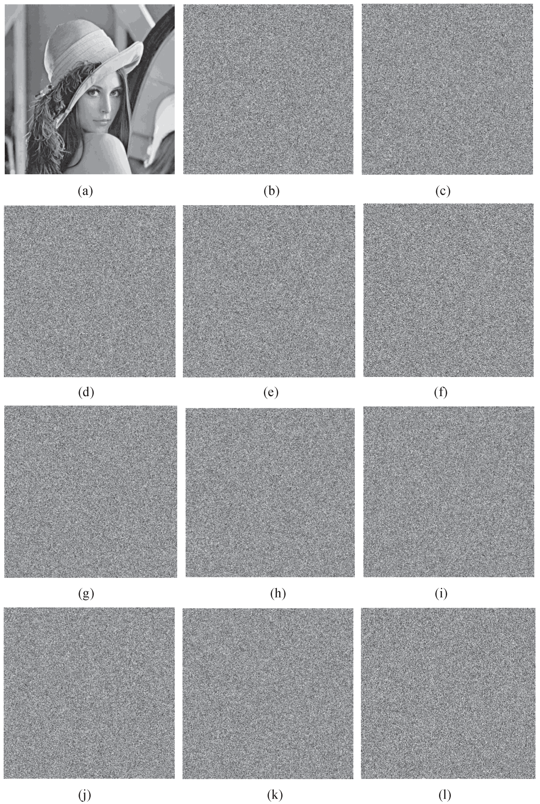
4.7. Key Sensitivity Analysis

According to the Kerckhoff’s principle, the randomness of cryptographic keys decides the security level of the image encryption algorithms. So, in order to hold the high security, the proposed image encryption algorithm must be very sensitive to the cryptographic keys. It means a trivial change in the cryptographic keys must get enormously different encrypted or decrypted image. In this section, we provide key sensitivity analysis through trivial change in the encrypted key and decrypted key, respectively.

4.7.1. Encrypted Key Sensitivity Analysis

Here, we represent the secret key of the proposed algorithm as $(A,B)$, where $A=(x_0^{\prime },x_1^{\prime },x_2^{\prime },\cdots ,x_{10}^{\prime })$, $B=(k_0^{\prime },k_1^{\prime },k_2^{\prime },\cdots ,k_{10}^{\prime })$. In the following, we make a slight modification on the 12 groups encrypted keys to one of the parameters with others remain unchanged, the detailed 12 groups encrypted keys are listed as follows:

$Ke{y}_1$:

A = (0.34556788,0.13456790, 0.24567981, 0.34567932, 0.42345679, 0.53456794, 0.64567958, 0.76456793, 0.86456797,0.754712846, 0.567889322), B = (π, 8, 7, 6, 5, 4, 3, 2, 13,11,10).

$Ke{y}_2$:

A = (0.34556789,0.13456790, 0.24567981, 0.34567932, 0.42345679, 0.53456794, 0.64567958, 0.76456793, 0.86456797,0.754712846, 0.567889322), B = (π, 8, 7, 6, 5, 4, 3, 2, 13,11,10).

$Ke{y}_3$:

A = (0.34556788, 0.13456791, 0.24567981, 0.34567932, 0.42345679, 0.53456794, 0.64567958, 0.76456793, 0.86456797,0.754712846, 0.567889322), B = (π, 8, 7, 6, 5, 4, 3, 2, 13,11,10).

$Ke{y}_4$:

A = (0.34556788,0.13456790, 0.24567982, 0.34567932, 0.42345679, 0.53456794, 0.64567958, 0.76456793, 0.86456797,0.754712846, 0.567889322), B = (π, 8, 7, 6, 5, 4, 3, 2, 13,11,10).

$Ke{y}_5$:

A = (0.34556788,0.13456790, 0.24567981, 0.34567931, 0.42345679, 0.53456794, 0.64567958, 0.76456793, 0.86456797,0.754712846, 0.567889322), B = (π, 8, 7, 6, 5, 4, 3, 2, 13,11,10).

$Ke{y}_6$:

A = (0.34556788,0.13456790, 0.24567981, 0.34567932, 0.42345680, 0.53456794, 0.64567958, 0.76456793, 0.86456797,0.754712846, 0.567889322), B = (π, 8, 7, 6, 5, 4, 3, 2, 13,11,10).

$Ke{y}_7$:

A = (0.34556788,0.13456790, 0.24567981, 0.34567932, 0.42345679, 0.53456795, 0.64567958, 0.76456793, 0.86456797,0.754712846, 0.567889322), B = (π, 8, 7, 6, 5, 4, 3, 2, 13,11,10).

$Ke{y}_8$:

A = (0.34556788,0.13456790, 0.24567981, 0.34567932, 0.42345679, 0.53456794, 0.64567959, 0.76456793, 0.86456797,0.754712846, 0.567889322), B = (π, 8, 7, 6, 5, 4, 3, 2, 13,11,10).

$Ke{y}_9$:

A = (0.34556788,0.13456790, 0.24567981, 0.34567932, 0.42345679, 0.53456794, 0.64567958, 0.76456794, 0.86456797,0.754712846, 0.567889322), B = (π, 8, 7, 6, 5, 4, 3, 2, 13,11,10)

$Ke{y}_{10}$:

A = (0.34556788,0.13456790, 0.24567981, 0.34567932, 0.42345679, 0.53456794, 0.64567958, 0.76456793, 0.86456798, 0.754712846, 0.567889322), B = (π, 8, 7, 6, 5, 4, 3, 2, 13,11,10)

$Ke{y}_{11}$:

A = (0.34556788,0.13456790, 0.24567981, 0.34567932, 0.42345679, 0.53456794, 0.64567958, 0.76456793, 0.86456797, 0.754712847, 0.567889322), B = (π, 8, 7, 6, 5, 4, 3, 2, 13,11,10)

$Ke{y}_{12}$:

A = (0.34556788,0.13456790, 0.24567981, 0.34567932, 0.42345679, 0.53456794, 0.64567958, 0.76456793, 0.86456797, 0.754712846, 0.567889323), B = (π, 8, 7, 6, 5, 4, 3, 2, 13,11,10)

Then, we encrypt the plain image with the 12 groups keys by the proposed scheme, respectively, and the encrypted images are listed in Figure 7a–l.

Moreover, we compute the differences among Figure 7a–l in

Table 8. The encrypted key sensitivity analysis.

$\mathit{K}$	${\mathit{K}\mathit{e}\mathit{y}}_{\mathbf{1}}$	${\mathit{K}\mathit{e}\mathit{y}}_{\mathbf{2}}$	${\mathit{K}\mathit{e}\mathit{y}}_{\mathbf{3}}$	${\mathit{K}\mathit{e}\mathit{y}}_{\mathbf{4}}$	${\mathit{K}\mathit{e}\mathit{y}}_{\mathbf{5}}$	${\mathit{K}\mathit{e}\mathit{y}}_{\mathbf{6}}$	${\mathit{K}\mathit{e}\mathit{y}}_{\mathbf{7}}$	${\mathit{K}\mathit{e}\mathit{y}}_{\mathbf{8}}$	${\mathit{K}\mathit{e}\mathit{y}}_{\mathbf{9}}$	${\mathit{K}\mathit{e}\mathit{y}}_{\mathbf{10}}$	${\mathit{K}\mathit{e}\mathit{y}}_{\mathbf{11}}$	${\mathit{K}\mathit{e}\mathit{y}}_{\mathbf{12}}$
$Ke{y}_1$	0	0.99617	0.99600	0.99207	0.98381	0.96877	0.93839	0.97691	0.97549	0.97625	0.99577	0.99630
$Ke{y}_2$	0.99617	0	0.99631	0.99622	0.99599	0.99621	0.99612	0.99609	0.99616	0.99599	0.99588	0.99615
$Ke{y}_3$	0.99600	0.99631	0	0.99613	0.99635	0.99619	0.99614	0.99597	0.99611	0.99609	0.99611	0.99604
$Ke{y}_4$	0.99207	0.99622	0.99613	0	0.99246	0.99254	0.99178	0.99192	0.99210	0.99217	0.99598	0.99597
$Ke{y}_5$	0.98381	0.99599	0.99635	0.99246	0	0.98441	0.98413	0.98443	0.98447	0.98463	0.99611	0.99612
$Ke{y}_6$	0.96877	0.99621	0.99619	0.99254	0.98441	0	0.96814	0.96885	0.96847	0.96888	0.99614	0.99615
$Ke{y}_7$	0.93839	0.99612	0.99614	0.99178	0.98413	0.96814	0	0.93682	0.93850	0.93759	0.99593	0.99614
$Ke{y}_8$	0.97691	0.99609	0.99597	0.99192	0.98443	0.96885	0.93682	0	0.95173	0.90193	0.99608	0.99616
$Ke{y}_9$	0.97549	0.99616	0.99611	0.99210	0.98447	0.96847	0.93850	0.95173	0	0.95015	0.99604	0.99623
$Ke{y}_{10}$	0.97625	0.99599	0.99609	0.99217	0.98463	0.96888	0.93759	0.90193	0.95015	0	0.99617	0.99622
$Ke{y}_{11}$	0.99577	0.99588	0.99611	0.99598	0.99611	0.99614	0.99593	0.99608	0.99604	0.99617	0	0.99606
$Ke{y}_{12}$	0.99630	0.99615	0.99604	0.99597	0.99612	0.99615	0.99614	0.99616	0.99623	0.99622	0.99606	0

. All the graph and computation results demonstrate that the proposed algorithm is quite sensitive to the encrypted key.

4.7.2. Decrypted Key Sensitivity Analysis

Furthermore, because the proposed algorithm is a symmetric cipher, so, we decrypt Figure 7a with the same secret keys $Ke{y}_1$ in Figure 8a. In order to show that the proposed algorithm is sensitive to the decrypted key, we also use $Ke{y}_2,\cdots ,Ke{y}_{12}$ to decrypt Figure 7a, respectively, and draw the decrypted images in Figure 8b–l, respectively. The results of the differences between the right decrypted image (Figure 1a) and the wrong decrypted images ( Figure 1b–l are 0.996090, 0.996162, 0.996437, 0.996117, 0.995964, 0.996193, 0.996142, 0.995922, 0.992017, 0.991432, 0.996262, respectively. So, we can see that the proposed algorithm is also highly sensitive to the decrypted key.

Note that in the key sensitivity analysis, we do not test the sensitivity of the secret keys B because the sensitivities of B have been tested in Section 2.2. In conclusion, the proposed algorithm is highly sensitive to secret keys.

4.8. Chosen/Known Plaintext Attacks Analysis

Chosen/known plaintext attacks analysis is efficient and widely used security attack models in cryptanalysis. The former assumes that the attackers have the ability to choose arbitrary plaintexts and obtain the corresponding cipher texts. So, the attackers can disclose the relation between the plaintexts and ciphertexts, and even deduce the secret key if the encryption structure is not sufficiently secure. Many successful cryptanalysis cases using the chosen/known plaintext attack were reported in [31,32,33,40]. In the proposed algorithm, special structures are designed to resist the chosen or known plaintext attacks: Firstly, the principle of confusion and diffusion introduced by Shannon are fulfilled. A bit of a pixel in the plain image can be permuted to any position and a small change can be spread overall pixels in the cipher image. Moreover, better diffusion effect are realized with the proposed bit-level permutation and pixel-level diffusion. Most important, random values and the total information of the plain image are added into the diffusion procedure. As a result, the obtained cipher images are totally different even using the same secret key to encrypt different plain image several times.

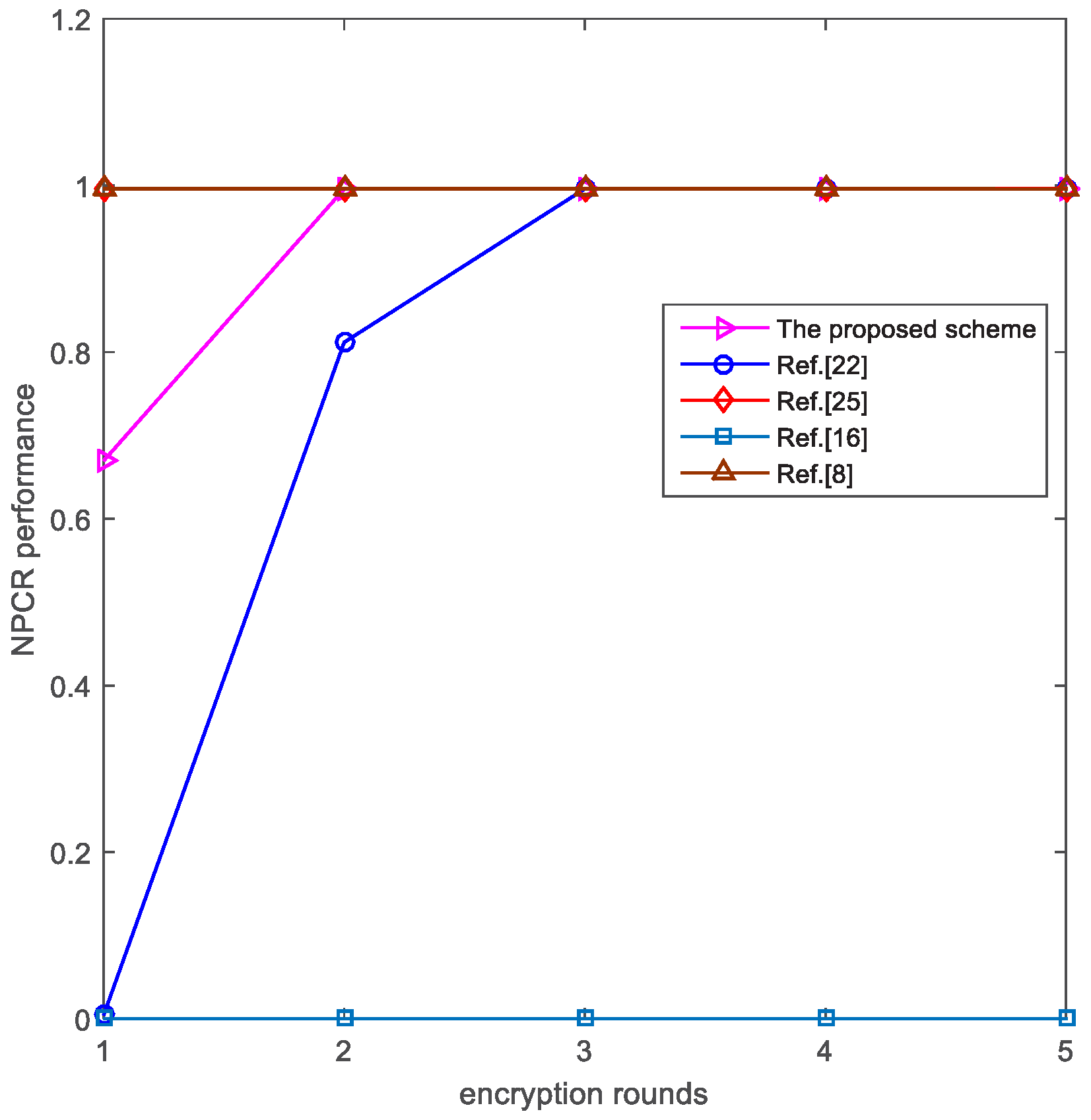
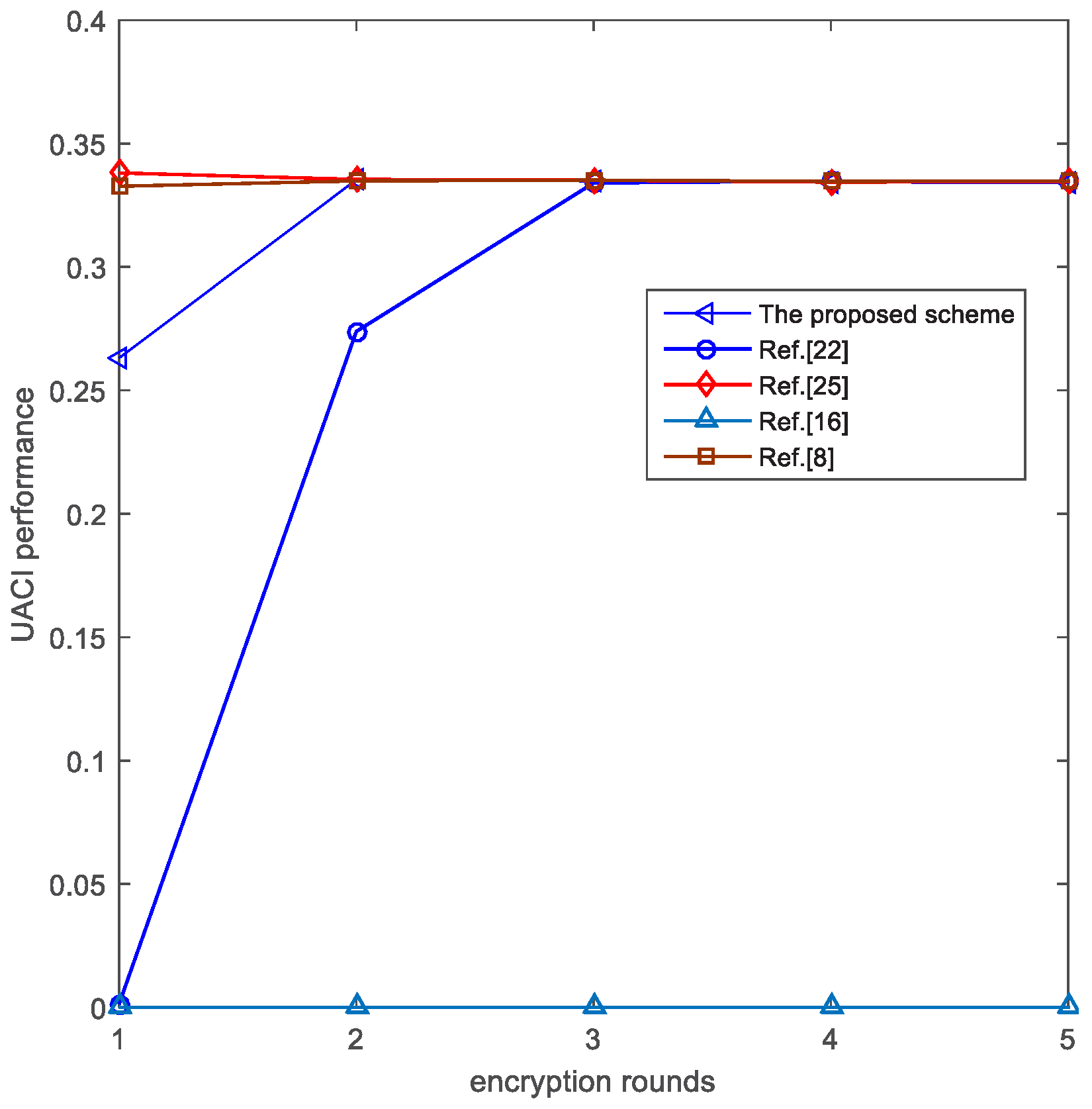
4.9. Differential Attack Analysis

The encryption scheme should be sensitive to a trivial change (e.g., modify only one pixel value or a bit) in the plain image. Two common measures are used: one is the number of pixels change rate (NPCR) and the other is the unified average changing intensity (UACI). NPCR measures the percentage of different pixel numbers between the two encrypted images, and UACI measures the average intensity of differences between two encrypted images. Let $C_1$, $C_2$ be two encrypted images, whose corresponding plain images have only one different pixel value. The NPCR and UACI are defined by the following Equations (16)–(18):

$$NPCR=\sum _{i,j}\frac{d(i,j)}{h\times w}$$

(16)

$$d(i,j)=\left\{\begin{array}{c}1C_1(i,j)\ne C_2(i,j)\hfill \\ 0otherwise\hfill \end{array}\right.$$

(17)

$$UACR=\frac{1}{h\times w}\sum _{i,j}\frac{|c_1(i,j)-c_2(i,j)|}{255}$$

(18)

where h and w are the height and width of the plain image, respectively.

Two plain images are used in the test. The first image is the original Lena image, and the other is obtained by changing the pixel value in the top left corner from “10100010” to “10100001’ (just a bit change). Then the two images are encrypted with the same secret keys for a few rounds to generate the corresponding cipher images $C_1$ and $C_2$. The results are listed in

Table 9. NPCR Performance.

Round	The Proposed Scheme	Ref. [16]	Ref. [22]	Ref. [8]	Ref. [25]
1	0.6696014404	0.000015259	0.00654386	0.9960098267	0.9963431625
2	0.995967865	0.000015259	0.80495842	0.9960746765	0.9959527564
3	0.9961090088	0.000015259	0.99615466	0.9961242676	0.9965357538
4	0.9961585999	0.000015259	0.99595247	0.9961776733	0.9960346326
5	0.9961013794	0.000015259	0.99616793	0.9959716797	0.9961644326

and

Table 10. UACI Performance.

Round	The Proposed Scheme	Ref. [16]	Ref. [22]	Ref. [8]	Ref. [25]
1	0.2630562577	0.000012087	0.00321365	0.3326689627	0.3360676146
2	0.3353189655	0.000012087	0.24366436	0.3348488303	0.335123463
3	0.3346790837	0.000012087	0.33401162	0.3351597805	0.3350163487
4	0.3342736338	0.000012087	0.33389708	0.3346462175	0.3344254165
5	0.3340085647	0.000012087	0.33441636	0.3348087535	0.3343425278

, respectively.

They indicate that NPCR and UACI of the proposed scheme can reach 0.995967865 and 0.3353189655 in the second encryption round, respectively, We note that it is a little lower than Ref. [8], which has good performance in the first encryption round, but it is better than that of Refs. [16], [22] and [25]. Therefore, the proposed scheme is very sensitive to even 1 bit modification in the plain image. Furthermore, to show these growing trends graphically, the NPCR and UACI data with 5 rounds are plotted in Figure 9 and Figure 10, respectively.

4.10. Randomness Analysis of CDCS

As we know, according to the Kerckhoff’s principle, the randomness level of cryptographic keystream decides the security level of the cipher algorithms. In this subsection, we evaluate the performances of CDCS by the NIST SP 800-22 tests [41]. In NIST SP 800-22 tests, each test produces a p-value which is a real number in $[0,1]$. If the p-value is greater than a predefined significant level α, it means the random sequence can pass the test successfully. In our experiment, we set α = 0.01. The test results are listed in

Table 11. The test result of NIST SP 800-22 tests for CDCS.

Test Name	p-value	Results
Frequency test	0.5731	Success
Block Frequency test	0.6825	Success
Cusum-Forward test	0.9293	Success
Cusum-Reverse test	0.3514	Success
Runs test	0.5536	Success
Long Runs test of Ones	0.6154	Success
Binary Matrix Rank Test	0.7635	Success
Spectral DFT test	0.4674	Success
Non-overlapping test Templates (m = 9, B = 000000001)	0.8710	Success
Overlapping test Templates (m = 9)	0.9241	Success
Maurer’s Universal test (L = 7, Q = 1280)	0.3533	Success
Approximate Entropy test (m = 5)	0.9987	Success
Random Excursions test (x = +1)	0.2085	Success
Lempel Ziv compression test	0.6784	Success
Linear complexity test	0.2314	Success
Random Excursions Variant test (x = −1)	0.5811	Success
Serial test (m = 5,$\nabla {\phi }_m^2$)	0.8989	Success

. From Table 11, CDCS pass NIST SP 800-22 tests and exhibit excellent statistical properties. Thus, CDCS provides a better choice for image encryption algorithm.

4.11. Speed Performance

Except for the security consideration, the running speed is another important factor for a good image encryption algorithm. Obviously, the proposed algorithm is the classic permutation-diffusion framework, and it consist of a bit-level permutation procedure and a pixel-level diffusion procedure. So, we show speed performance with permutation time and diffusion time, respectively. From

Table 12. Speed Performance (seconds).

Time (s)	The Proposed Scheme	Ref. [16]	Ref. [22]	Ref. [8]	Ref. [25]
permutation time	10.647093	0.603354	9.789038	0.758742	14.161442
diffusion time	0.648852	0.55907	1.018693	–	2.8315003
total time	10.3959	1.1624	10.8077	0.758742	16.9929

, the bit-level permutation time of the proposed algorithm is lower than the two bit-level permutation algorithms in [22,25]. Because the bit-level operation need more time than the pixel-level operation, so, the permutation operation time is larger than the pixel-level permutation algorithms in [8,16], and the diffusion time is acceptable.

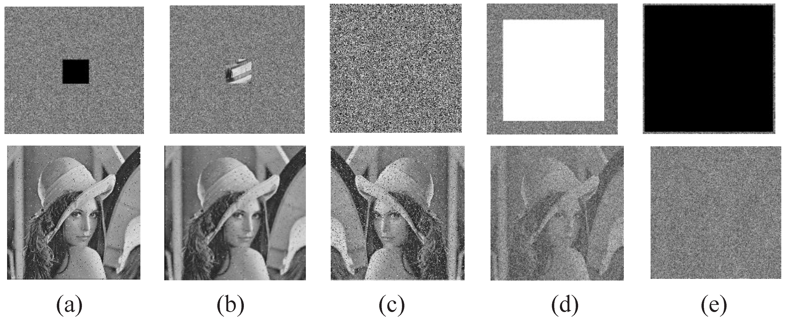
4.12. Robustness of the Proposed Algorithm in Noise and Data Loss

Digital images are usually transmitted in the public networks, and the encryption algorithm is usual open. So, the attackers can choose special plain images for encryption and try to find the secret key. So, a secure image encryption algorithm should resist this attacks. The secret key of the proposed algorithm consist of some random values and the total information of the plain image, so, even the attackers choose some special image to encrypt, and get some information of the secret key, but it can not get the right decrypted image, because the initial value of $te{m}_0,te{m}_1$ are different, so the random sequence used in the diffusion procedure Equation (12) will be absolutely different.

Moreover, the attackers can disguise the legal user to obtain the cipher image, tamper with the intermediate form of the proposed algorithm more convenient, then information loss and pixel value modification of digital images may happen. Here we show the robustness of the proposed algorithm in noise and data loss, which means that if a portion of pixels in the cipher image are modified or lost, the original image can still be reconstructed with a acceptable visual quality. Figure 11 shows the proposed algorithm can resist the noise and data loss attacks in a high level.

5. Conclusions

In this paper, we propose a new two dimensional composite discrete chaotic system-based image encryption scheme, and use the new CDCS to accomplish the bit-level permutation and pixel-level diffusion. Simulation results show the security and the validity of the proposed scheme with the several characters: (1) The CDCS has excellent chaotic behaviors because it combines two single chaotic system in a random way. (2) It has a bit-level permutation and pixel-level diffusion architecture where the image is encrypted with a single-permutation and double-diffusion effect with only scan the plain image one time. (3) the value of the ciphered pixel influenced the next pixel’s permutation and diffusion effect, and a pixel in the plain image can be permuted to any position and a small change can be spread overall pixels in the cipher image.

However, in the bit-level permutation stage, the proposed image encryption algorithm need to change each pixel value into a 8 bits sequence, which means that the operation time is longer than the pixel-level image encryption algorithms. The speed performance in Section 4.11 verifies this conclusion.

In future, considering the excellent chaotic behaviors of the high-dimensional chaos map and hyper chaos. With the good structure of the composite discrete chaotic system, we can design composite discrete high-dimensional chaotic system and composite hyper-chaotic dynamical system to enhance the complex of the chaotic system and obtain excellent chaos, but we should consider the time consuming and convenience when use these systems in image encryption.

References

1. Fridrich, J. Symmetric ciphers based on two-dimensional chaotic maps. Int. J. Bifurc. Chaos 1998, 8, 1259–1284. [Google Scholar] [CrossRef]
2. Ye, G. Image scrambling encryption algorithm of pixel bit based on chaos map. Pattern Recognit. Lett. 2014, 31, 347–354. [Google Scholar]
3. Norouzi, B.; Mirzakuchaki, S. A fast color image encryption algorithm based on hyper-chaotic systems. Nonlinear Dyn. 2014, 78, 995–1015. [Google Scholar] [CrossRef]
4. Baptista, M.S. Cryptography with chaos. Phys. Lett. A 1998, 240, 50–54. [Google Scholar] [CrossRef]
5. Wang, X.Y.; Zhang, Y.Q.; Bao, X.M. A colour image encryption scheme using permutation-substitution based on chaos. Entropy 2015, 17, 3877–3897. [Google Scholar] [CrossRef]
6. Murillo-Escobar, M.A.; Cruz-Hernandez, C.; Abundiz-Perez, F.; Lopez-Gutierrez, R.M.; del Campo, O.A. A RGB image encryption algorithm based on total plain image characteristics and chaos. Signal Process. 2015, 109, 119–131. [Google Scholar] [CrossRef]
7. Zheng, Y.; Jin, J. A novel image encryption scheme based on Henon map and compound spatiotemporal chaos. Multimed. Tools Appl. 2014, 74, 7803–7820. [Google Scholar] [CrossRef]
8. Zhou, Y.; Bao, L.; Philip Chen, C.L. Image encryption using a new parametric switching chaotic system. Signal Process. 2013, 93, 3039–3052. [Google Scholar] [CrossRef]
9. Liu, W.; Sun, K.; Zhu, C. A fast image encryption algorithm based on chaotic map. Opt. Lasers Eng. 2016, 84, 26–36. [Google Scholar] [CrossRef]
10. Hua, Z.; Zhou, Y.; Pun, C.-M.; Philip Chen, C.L. 2D Sine Logistic modulation map for image encryption. Inf. Sci. 2015, 297, 80–94. [Google Scholar] [CrossRef]
11. Hua, Z.; Zhou, Y. Image encryption using 2D Logistic-adjusted-Sine map. Inf. Sci. 2016, 339, 237–253. [Google Scholar]
12. Mollaeefar, M.; Sharif, A.; Nazari, M. A novel encryption scheme for colored image based on high level chaotic maps. Multimed. Tools Appl. 2015, 74, 1–23. [Google Scholar] [CrossRef]
13. Wang, X.; Zhang, H. A novel image encryption algorithm based on genetic recombination and hyper-chaotic systems. Nonlinear Dyn. 2015, 83, 333–346. [Google Scholar] [CrossRef]
14. Wu, X.; Wang, D.; Kurths, J.; Kan, H. A novel lossless color image encryption scheme using 2D DWT and 6D hyperchaotic system. Inf. Sci. 2016, 349, 137–153. [Google Scholar] [CrossRef]
15. Wu, X.; Bai, C.; Kan, H. A new color image cryptosystem via hyperchaos synchronization. Commun. Nonlinear Sci. Numer. Simul. 2014, 19, 1884–1897. [Google Scholar] [CrossRef]
16. Zhu, H.; Zhao, C.; Zhang, X. A novel image encryption-compression scheme using hyper-chaos and Chinese remainder theorem. Signal Process. Image Commun. 2013, 28, 670–680. [Google Scholar] [CrossRef]
17. Tong, X.; Wang, Z.; Liu, Y.; Zhang, M.; Xu, L. A novel compound chaotic block cipher for wireless sensor networks. Commun. Nonlinear Sci. Numer. Simul. 2015, 22, 120–133. [Google Scholar] [CrossRef]
18. Wang, L.; Song, H.; Liu, P. A novel hybrid color image encryption algorithm using two complex chaotic systems. Opt. Lasers Eng. 2016, 77, 118–125. [Google Scholar] [CrossRef]
19. Tong, X.; Zhang, M.; Wang, Z.; Liu, Y. An image encryption scheme based on dynamical perturbation and linear feedback shift register. Nonlinear Dyn. 2014, 78, 2277–2291. [Google Scholar] [CrossRef]
20. Tong, X.; Cui, M. Image encryption scheme based on 3d baker with dynamical compound chaotic sequence cipher generator. Signal Process. 2009, 89, 480–491. [Google Scholar] [CrossRef]
21. Tong, X. The novel bilateral-diffusion image encryption algorithm with dynamical compound chaos. J. Syst. Softw. 2012, 85, 850–859. [Google Scholar] [CrossRef]
22. Zhu, Z.; Zhang, W.; Wong, K.W.; Yu, H. A chaos-based symmetric image encryption scheme using a bit-level permutation. Inf. Sci. 2011, 181, 1171–1186. [Google Scholar] [CrossRef]
23. Zhang, W.; Yu, H.; Zhao, Y.; Zhu, Z. Image encryption based on three-dimensional bit matrix permutation. Signal Process. 2016, 118, 36–50. [Google Scholar] [CrossRef]
24. Fu, C.; Huang, J.B.; Wang, N.N.; Hou, Q.B.; Lei, W.M. A Symmetric chaos-based image cipher with an improved bit-Level permutation strategy. Entropy 2014, 16, 770–788. [Google Scholar] [CrossRef]
25. Zhu, H.; Zhao, C.; Zhang, X.; Yang, L. An image encryption scheme using generalized Arnold map and affine cipher. Optik 2014, 125, 6672–6677. [Google Scholar] [CrossRef]
26. Wang, X.; Luan, D. A novel image encryption algorithm using chaos and reversible cellular automata. Commun. Nonlinear Sci. Numer. Simul. 2013, 18, 3075–3085. [Google Scholar] [CrossRef]
27. Song, C.; Qiao, Y. A novel image encryption algorithm based on DNA encoding and spatiotemporal chaos. Entropy 2015, 17, 6954–6968. [Google Scholar] [CrossRef]
28. Wu, X.; Kan, H.; Kurths, J. A new color image encryption scheme based on DNA sequences and multiple improved 1D chaotic maps. Appl. Soft. Comput. 2015, 37, 24–39. [Google Scholar] [CrossRef]
29. Ye, G. A block image encryption algorithm based on wave transmission and chaotic systems. Nonlinear Dyn. 2014, 75, 417–427. [Google Scholar] [CrossRef]
30. Li, C.; Liu, Y.; Xie, T.; Chen, M. Breaking a novel image encryption scheme based on improved hyperchaotic sequences. Nonlinear Dyn. 2013, 73, 2083–2089. [Google Scholar] [CrossRef]
31. Jeng, F.G.; Huang, W.L.; Chen, T.H. Cryptanalysis and improvement of two hyper-chaos-based image encryption schemes. Signal Process. Image Commun. 2015, 34, 45–51. [Google Scholar] [CrossRef]
32. Li, C.; Lo, K.T. Optimal quantitative cryptanalysis of permutation-only multimedia ciphers against plaintext attacks. Signal Process. 2011, 91, 949–954. [Google Scholar] [CrossRef]
33. Li, C. Cracking a hierarchical chaotic image encryption algorithm based on permutation. Signal Process. 2015, 118, 203–210. [Google Scholar] [CrossRef]
34. Li, C.; Li, S.; Lo, K.T. Breaking a modified substitution-diffusion image cipher based on chaotic standard and logistic maps. Commun. Nonlinear Sci. Numer. Simul. 2011, 16, 37–843. [Google Scholar] [CrossRef] [Green Version]
35. Seyedzadeh, S.M.; Mirzakuchaki, S. A fast color image encryption algorithm based on coupled two-dimensional piecewise chaotic map. Signal. Process. 2012, 92, 1202–1215. [Google Scholar] [CrossRef]
36. Liu, H.; Wang, X. Triple-image encryption scheme based on one-time key stream generated by chaos and plain images. J. Syst. Softw. 2013, 86, 826–834. [Google Scholar] [CrossRef]
37. Gottwald, G.A.; Melbourne, I. A new test for chaos in deterministic systems. Proc. R. Soc. Lond. A 2004, 460, 603–611. [Google Scholar] [CrossRef]
38. The USC-SIPI Image Database. Available online: http://sipi.usc.edu/database/database.php?volume=misc (accessed on 25 July 2016).
39. Wu, Y.; Zhou, Y.; Saveriades, G.; Agaian, S.; Noonan, J.P.; Natarajan, P. Local Shannon entropy measure with statistical tests for image randomness. Inf. Sci. 2013, 222, 323–342. [Google Scholar] [CrossRef]
40. Zhang, Y.; Xiao, D. Cryptanalysis of S-box-only chaotic image ciphers against chosen plaintext attack. Nonlinear Dyn. 2013, 72, 751–756. [Google Scholar]
41. A Statistical Test Suite for Random and Pseudorandom Number Generators for Cryptographic Applications. Available online: http://csrc.nist.gov/publications/nistpubs/800-22-rev1a/SP800-22rev1a.pdf (accessed on 10 April 2016).
Figure 1. The diffused images by different control parameter k of CDCS. (a) Lena image; (b) k = 2; (c) k = 3; (d) k = 4; (e) k = 5; (f) k = 6; (g) k = 7.
Entropy 18 00276 g001
Figure 2. Trajectories of different chaotic maps. (a) CDCS; (b) single discrete dynamic chaotic system Equation (3); (c) Logistic map.
Entropy 18 00276 g002
Figure 3. The proposed image encryption architecture.
Entropy 18 00276 g003
Figure 4. The histogram distribution analysis. (a) Plain image; (b) The histogram distribution of (a); (c) Permutated image; (d) The histogram distribution of (c); (e) Cipher image; (f) The histogram distribution of (e).
Entropy 18 00276 g004
Figure 5. Color image encryption effect. (a) House image; (b) The corresponding cipher image of (a); (c) Peppers image; (d) The corresponding cipher of (c).
Entropy 18 00276 g005
Figure 6. The correlation analyses of the proposed algorithms. (a) Horizontal direction of plain image lena; (b) Horizontal direction of cipher image; (c) Vertical direction of plain image; (d) Vertical direction of cipher image; (e) Diagonal direction of plain image; (f) Diagonal direction of cipher image.
Entropy 18 00276 g006
Figure 7. Encrypted key sensitivity analysis. (a) K e y 1 ; (b) K e y 2 ; (c) K e y 3 ; (d) K e y 4 ; (e) K e y 5 ; (f) K e y 6 ; (g) K e y 7 ; (h) K e y 8 ; (i) K e y 9 ; (j) K e y 10 ; (k) K e y 11 ; (l) K e y 12 .
Entropy 18 00276 g007
Figure 8. Decrypted key sensitivity analysis. (a) K e y 1 ; (b) K e y 2 ; (c) K e y 3 ; (d) K e y 4 ; (e) K e y 5 ; (f) K e y 6 ; (g) K e y 7 ; (h) K e y 8 ; (i) K e y 9 ; (j) K e y 10 ; (k) K e y 11 ; (l) K e y 12 .
Entropy 18 00276 g008
Figure 9. NPCR analysis.
Entropy 18 00276 g009
Figure 10. UACI analysis.
Entropy 18 00276 g010
Figure 11. Robustness analysis results. (a) 3.6% data loss with a black square; (b) 3.6% data modification with a square; (c) 5% Salt and Pepper noise; (d) 60.12% data loss with a white square; (e) 94.23% data loss with a black square.
Entropy 18 00276 g011