Complex Dynamics of a Continuous Bertrand Duopoly Game Model with Two-Stage Delay

Abstract

This paper studies a continuous Bertrand duopoly game model with two-stage delay. Our aim is to investigate the influence of delay and weight on the complex dynamic characteristics of the system. We obtain the bifurcation point of the system respect to delay parameter by calculating. In addition, the dynamic properties of the system are simulated by power spectrum, attractor, bifurcation diagram, the largest Lyapunov exponent, 3D surface chart, 4D Cubic Chart, 2D parameter bifurcation diagram, and 3D parameter bifurcation diagram. The results show that the stability of the system depends on the delay and weight, in order to maintain stability of price and ensure the firm profit, the firms must control the parameters in the reasonable region. Otherwise, the system will lose stability, and even into chaos, which will cause fluctuations in prices, the firms cannot be profitable. Finally, the chaos control of the system is carried out by a control strategy of the state variables’ feedback and parameter variation, which effectively avoid the damage of chaos to the economic system. Therefore, the results of this study have an important practical significance to make decisions with multi-stage delay for oligopoly firms.

1. Introduction

When the market is supplied by only a few firms, oligopolistic competition is easy to occur where they produce homogeneous goods in the same market. In fact, the firms make optimal decisions for the maximization of profit. In this paper, we consider a firm that adopts a delay strategy, which refers to two different historical prices, to make a decision. Another firm makes a decision without delay. The Bertrand model considers a duopoly with a single homogeneous product, which has been studied in many papers. Some researchers have studied the Bertrand duopoly with differentiated products. The results show that the degree of product differentiation has a great influence on the price and quantity of sale [1,2,3]. In the Bertrand game model, the amount of information that the duopoly has will affect the stability of the system, mainly reflected in the change of the basin of attraction [4]. In order to maximize profits, the duopoly enterprise launches a price competition and expands market share. However, this will have a greater impact on the dynamics of the game model [5,6,7], having studied the price competition and chaos control of the air conditioning market. They focused on the role of coordination and distributed demand in price competition in the air conditioner market. Since the market information is not complete, the duopoly enterprise must adopt bounded rationality for a price decision. The scholars have studied the complexity of the game model with bounded rationality about synchronization, marginal costs, and so on [8,9,10]. The duopoly enterprise makes price decisions not only in reference to the current price but also in reference to historical prices. The effect of two-stage delay on the complexity of the system is studied in [11,12], and the stability region of the system is given. The nonlinear dynamic behavior of the triopoly game model is studied from heterogeneous and delayed bounded rationality, respectively, in [13,14]. The research conclusions are the same as that of a two-dimensional game model, but the research process is more complex. Scholars have studied not only the Bertrand game model, but also investigated the complexity of the Cournot game model, the Stackelberg game model and the Holling–Tanner model. Their research methods are useful for reference in this paper [15,16,17].

In short, most of the studies are discrete, and there are very few with respect to two-stage delay. In this paper, we establish a continuous Bertrand duopoly game model with two-stage delay. We focus on the influence of delay parameters on the dynamic characteristics of the system.

This paper is organized as follows: in Section 2, a continuous differential Bertrand duopoly game mode with two-stage delay is established. The process solution of delay is given, and studies the influence of delay on the stability of the system. In Section 3, numerical simulation is conducted, through the attractor, bifurcation diagram, the largest Lyapunov exponent, and initial value sensitivity, etc., to study the influence of delay and weight on the stability of price and profit. In Section 4, the effective control of chaos by a feedback control method is adopted in the system. Finally, the conclusion of this paper is provided in the last section.

2. The Model

In this part, we study the influence of delay on the dynamics of the system when the economic system is composed of two firms. Let us assume they produce similar products. Let $p_i$ denote the price of product i and $q_i$ denote the demand of product i (i = 1, 2). We assume demand function is linear form:

$$\{\begin{array}{l}{q}_1=a_1-b_1{p}_1+d_1{p}_2\\ q_2=a_2-b_2{p}_2+d_2{p}_1\end{array}$$

(1)

where $a_i$, $b_i$, $d_i>0$ (i = 1, 2), $a_i$ are the basic demand for the market, $b_i$ denotes the elastic demand for itself and $d_i$ denotes the substitution rate between products. Where $c_i$ is constant are the marginal costs of Firm i [2]. Further, we assume linear cost function given by:

$$C_i(q_i)=c_i{q}_i,i=1,2$$

(2)

Then the profit of the i-th Firm becomes:

$$\{\begin{array}{l}{\pi }_1(p_1,p_2)=(p_1-c_1)(a_1-b_1{p}_1+d_1{p}_2)\\ {\pi }_2(p_1,p_2)=(p_2-c_2)(a_2-b_2{p}_2+d_2{p}_1)\end{array}$$

(3)

In such a way, we have a game in which the firms are a duopoly. In the real market, the information of the firms is not complete, and they exhibit bounded rationality when making decisions. Typically, the firm makes price decisions, not only considering the current profit margin, but also consider the profit margin before $\tau$, so that the final price is closer to the actual value of the product.

In this paper, we assume that Firm 1 implements a two-stage delay, that is to say, it refers to the historical price of two different periods, the delay parameters are ${\tau }_1$ and ${\tau }_2$. Firm 2 makes price decisions without delay. Since the current price cannot be obtained accurately, here we do not consider the current price. When making price decisions, Firm 1 only considers two historical prices. Thus, the dynamic process of decision is changed into:

$$\stackrel{·}{p_i}(t)={\alpha }_i(p_i)\frac{\partial {\pi }_i(p_1^d,p_2)}{\partial p_i}$$

(4)

where ${\alpha }_i(p_i)$ indicates the degree of change in the product price with the marginal profit. We assume that ${\alpha }_i(p_i)$ are a linear form ${\alpha }_i(p_i)={\nu }_i{p}_i$, $i=1,2$. Where ${\nu }_i({\nu }_i>0)$ indicates the speed of the price adjustment of Firm i.

$$p_1^d=w{p}_1(t-{\tau }_1)+(1-w)p_1(t-{\tau }_2)$$

(5)

where $0\le w\le 1$ is the price weight of $t-{\tau }_1$, $1-w$ is the price weight of $t-{\tau }_2$. From Equations (3)–(5), the dynamical system model with two-stage delay is as follows:

$$\{\begin{array}{l}\stackrel{·}{p_1}(t)={\nu }_1{p}_1(a_1-2b_{1}w{p}_1(t-{\tau }_1)-2b_1(1-w)p_1(t-{\tau }_2)+d_1{p}_2+b_1{c}_1)\\ \stackrel{·}{p_2}(t)={\nu }_2{p}_2(a_2-2b_2{p}_2+d_{2}w{p}_1(t-{\tau }_1)+d_2(1-w)p_1(t-{\tau }_2)+b_2{c}_2)\end{array}$$

(6)

3. Equilibrium Points and Local Stability

When the price competition of firms reaches equilibrium, we can get the following equilibrium point of Equation (6): $E_1(0,0)$, $E_2(0,\frac{a_2+b_2{c}_2}{2b_2})$, $E_3(\frac{a_1+b_1{c}_1}{2b_1},0)$, $E_4(p_1^{*},p_2^{*})$, where:

$$p_1^{*}=\frac{2a_1{b}_2+a_2{d}_1+2b_1{b}_2{c}_1+b_2{c}_2{d}_1}{4b_1{b}_2-d_1{d}_2},p_2^{*}=\frac{2a_2{b}_1+a_1{d}_2+2b_1{b}_2{c}_2+b_1{c}_1{d}_2}{4b_1{b}_2-d_1{d}_2}$$

According to the economic significance, the equilibrium point should be non-negative, so $E_1$, $E_2$, and $E_3$ are the boundary equilibrium points, and only $E_4$ is the Nash equilibrium point. It means that the price of firms can be stabilized in a state of equilibrium through competition. In this paper, we focus on the influence of ${\tau }_1$, ${\tau }_2$ and $w$ on the dynamic behavior of Equation (6) at the Nash equilibrium point.

The linearized Equation (6) at the equilibrium point $E_4(p_1^{*},p_2^{*})$ by Jacobian matrix is:

$$\{\begin{array}{l}\stackrel{·}{p_1}(t)=(a_1{\nu }_1-2b_1{\nu }_1{p}_1^{*}+d_1{\nu }_1{p}_2^{*}+b_1{c}_1{\nu }_1)p_1-2b_1{\nu }_{1}w{p}_1^{*}{p}_1(t-{\tau }_1)-2b_1{\nu }_1(1-w)p_1^{*}{p}_1(t-{\tau }_2)+d_1{\nu }_1{p}_1^{*}{p}_2\\ \stackrel{·}{p_2}(t)=d_2{\nu }_{2}w{p}_2^{*}{p}_1(t-{\tau }_1)+d_2{\nu }_2(1-w)p_2^{*}{p}_1(t-{\tau }_2)+(a_2{\nu }_2-4b_2{\nu }_2{p}_2^{*}+d_2{\nu }_2{p}_1^{*}+b_2{\nu }_2{c}_2)p_2\end{array}$$

(7)

The characteristic equation associated with Equation (7) is given by:

$$\left|\begin{array}{cc}\lambda -J_{11}\hfill & -J_{12}\\ -J_{21}\hfill & \lambda -J_{22}\end{array}\right|=0$$

(8)

where:

$$J_{11}=a_1{\nu }_1-2b_1{\nu }_1{p}_1^{*}+d_1{\nu }_1{p}_2^{*}+b_1{c}_1{\nu }_1-2b_1{\nu }_{1}w{p}_1^{*}{e}^{-\lambda {\tau }_1}-2b_1{\nu }_1(1-w)p_1^{*}{e}^{-\lambda {\tau }_2}$$

$$J_{12}=d_1{\nu }_1{p}_1^{*}$$

$$J_{21}=d_2{\nu }_{2}w{p}_2^{*}{e}^{-\lambda {\tau }_1}+d_2{\nu }_2(1-w)p_2^{*}{e}^{-\lambda {\tau }_2}$$

$$J_{22}=a_2{\nu }_2-4b_2{\nu }_2{p}_2^{*}+d_2{\nu }_2{p}_1^{*}+b_2{\nu }_2{c}_2$$

So we can get the characteristic equation for system Equation (7) as follows

$${\lambda }^2+A\lambda +(B\lambda +C)e^{-\lambda {\tau }_1}+(D\lambda +E)e^{-\lambda {\tau }_2}=0$$

(9)

where:

$$A=2b_2{p}_2^{*}{\nu }_2,B=2b_1{p}_1^{*}{\nu }_{1}w,C=4b_1{b}_2{p}_1^{*}{p}_2^{*}{\nu }_1{\nu }_{2}w-d_1{d}_2{p}_1^{*}{p}_2^{*}{\nu }_1{\nu }_{2}w$$

$$D=2b_1{p}_1^{*}{\nu }_1-2b_1{p}_1^{*}{\nu }_{1}w$$

$$E=4b_1{b}_2{p}_1^{*}{p}_2^{*}{\nu }_1{\nu }_2-d_1{d}_2{p}_1^{*}{p}_2^{*}{\nu }_1{\nu }_2-4b_1{b}_2{p}_1^{*}{p}_2^{*}{\nu }_1{\nu }_{2}w+d_1{d}_2{p}_1^{*}{p}_2^{*}{\nu }_1{\nu }_{2}w$$

3.1. Case 1. ${\tau }_1=0$, ${\tau }_2>0$

For ${\tau }_1=0$, the characteristic Equation (9) reduces to:

$${\lambda }^2+(A+B)\lambda +C+(D\lambda +E)e^{-\lambda {\tau }_2}=0$$

(10)

Let $\lambda =i{\omega }_2({\omega }_2>0)$ be the root of Equation (10). Separating the real and imaginary parts, we get the following:

$$\{\begin{array}{l}D{w}_{2}cos{w}_2{\tau }_2-Esin{w}_2{\tau }_2=-(A+B)w_2\\ Ecos{w}_2{\tau }_2+D{w}_{2}sin{w}_2{\tau }_2=w_2^2-C\end{array}$$

(11)

From (11), we can obtain:

$$\cos {\omega }_2{\tau }_2=\frac{(E-AD-BD){\omega }_2^2-CE}{D^2{\omega }_2^2+E^2}$$

(12)

Squaring both sides, adding both equations and regrouping by powers of ${\omega }_2$, we obtain that ${\omega }_2$ satisfies the following fourth degree polynomial:

$${\omega }_2^4+(A^2+B^2+2AB-2C-D^2){\omega }_2^2+C^2-E^2=0$$

(13)

In order to give the main results in this paper, we make the following assumption $(H_1)$: Equation (13) has at least one positive root ${\omega }_{20}$, which is:

$${\omega }_{20}=\sqrt{\frac{-(A^2+B^2+2AB-2C-D^2)+\sqrt{{(A^2+B^2+2AB-2C-D^2)}^2-4(C^2-E^2)}}{2}}$$

(14)

If condition $(H_1)$ holds, such that Equation (10) has a pair of purely imaginary roots $\pm i{\omega }_{20}$. The corresponding critical value of the delay by Equation (12) is:

$${\tau }_{20}=\frac{1}{{\omega }_{20}}\arccos \left[\frac{(E-AD-BD){\omega }_{20}^2-CE}{D^2{\omega }_{20}^2+E^2}\right]$$

(15)

Next, take the derivative with respect to ${\tau }_2$ in Equation (10), we can obtain:

$${\left[\frac{d\lambda }{d{\tau }_2}\right]}^{-1}=\frac{(2\lambda +A+B)e^{\lambda {\tau }_2}+D}{\lambda (D\lambda +E)}-\frac{{\tau }_2}{\lambda }$$

Thus:

$$\mathrm{Re}{\left[\frac{d\lambda ({\tau }_{20})}{d{\tau }_2}\right]}_{\lambda =i{\omega }_{20}}^{-1}=\frac{P_1{P}_3+P_2{P}_4}{P_1^2+P_2^2}$$

(16)

where:

$$P_1=-D{\omega }_{20}^2,P_2=E{\omega }_{20}$$

$$P_3=(A+B)\cos {\omega }_{20}{\tau }_{20}-2{\omega }_{20}\sin {\omega }_{20}{\tau }_{20}+D,P_4=2{\omega }_{20}\cos {\omega }_{20}{\tau }_{20}+(A+B)\sin {\omega }_{20}{\tau }_{20}$$

If condition $(H_2)$: $P_1{P}_3+P_2{P}_4\ne 0$, then $\mathrm{Re}{\left[\frac{d\lambda ({\tau }_{20})}{d{\tau }_2}\right]}_{\lambda =i{\omega }_{20}}^{-1}\ne 0$. According to the Hopf bifurcation theorem in [18], we obtain the following results.

Theorem 1. 

If the conditions $\left(H_1\right)$–$\left(H_2\right)$ hold, the equilibrium point $E_4(p_1^{*},p_2^{*})$ of Equation (6) is asymptotically stable for ${\tau }_2\in [0,{\tau }_{20})$ and unstable for ${\tau }_2>{\tau }_{20}$; Equation (6) undergoes a Hopf bifurcation when ${\tau }_2={\tau }_{20}$.

3.2. Case 2. ${\tau }_1>0$, ${\tau }_2>0$

In this case, we consider the characteristic Equation (9) with ${\tau }_2$ in its stable intervals, i.e., ${\tau }_2\in [0,{\tau }_{20})$ or ${\tau }_2\in [0,+\infty )$ [19]. We study the influence of ${\tau }_1$ on the stability of the system when ${\tau }_2$ fixed.

Let $\lambda =i{\omega }_1({\omega }_1>0)$ is a root of Equation (9). Then we obtain:

$$\{\begin{array}{l}B{\omega }_1\sin ({\omega }_1{\tau }_1)+C\cos ({\omega }_1{\tau }_1)={\omega }_1^2-E\cos ({\omega }_1{\tau }_2)-D{\omega }_1\sin ({\omega }_1{\tau }_2)\\ -C\sin ({\omega }_1{\tau }_1)+B{\omega }_1\cos ({\omega }_1{\tau }_1)=-A{\omega }_1-D{\omega }_1\cos ({\omega }_1{\tau }_2)+E\sin ({\omega }_1{\tau }_2)\end{array}$$

(17)

It follows from Equation (17) that:

$$\cos ({\omega }_1{\tau }_1)=\frac{m_1{\omega }_1^2+m_2{\omega }_1+m_3}{m_8},\sin ({\omega }_1{\tau }_1)=\frac{m_4{\omega }_1^3+m_5{\omega }_1^2+m_6{\omega }_1+m_7}{m_8}$$

with:

$$\begin{array}{l}{m}_1=C-AB-BD\cos ({\omega }_1{\tau }_2),m_2=BE\sin ({\omega }_1{\tau }_2)-CD\sin ({\omega }_1{\tau }_2)\\ m_3=-CE\cos ({\omega }_1{\tau }_2),m_4=B,m_5=-BD\sin ({\omega }_1{\tau }_2)\\ m_6=CD\cos ({\omega }_1{\tau }_2)-BE\cos ({\omega }_1{\tau }_2)+AC,m_7=-CE\sin ({\omega }_1{\tau }_2),m_8=B^2{\omega }_1^2+C^2\end{array}$$

Then we have:

$$n_6{\omega }_1^6+n_5{\omega }_1^5+n_4{\omega }_1^4+n_3{\omega }_1^3+n_2{\omega }_1^2+n_1{\omega }_1+n_0=0$$

(18)

where

$$\begin{array}{l}{n}_6=m_4^2,n_5=2m_4{m}_5,n_4=m_1^2+m_5^2+2m_4{m}_6,n_3=2m_1{m}_2+2m_4{m}_7+2m_5{m}_6\\ n_2=m_2^2+m_6^2+2m_1{m}_3+2m_5{m}_7,n_1=2m_2{m}_3+2m_6{m}_7,n_0=m_3^2+m_7^2-m_8\end{array}$$

Next, we give the following assumption $\left(H_3\right)$: Equation (18) has finite positive root. If $\left(H_3\right)$ holds, without loss of generality, we define the roots of Equation (18) as ${\omega }_{11},{\omega }_{12},\mathrm{...},{\omega }_{1k}$. Then, for every fixed ${\omega }_{1i}(i=1,2,\mathrm{...},k)$, there exists a sequence $\left\{{\tau }_{1i}^{(j)}|j=0,1,2,\mathrm{...}\right\}$ which satisfies Equation (18).

$${\tau }_{1i}^{(j)}=\frac{1}{{\omega }_{1i}}\arccos (\frac{m_1{\omega }_{1i}^2+m_2{\omega }_{1i}+m_3}{m_8})+\frac{2j\pi }{{\omega }_{1i}},i=1,2,\mathrm{...},k;j=0,1,\mathrm{2...}$$

(19)

Let ${\tau }_{10}=\min \{{\tau }_{1i}^{(j)}|j=0,1,2,\mathrm{...}\}=\min \{{\tau }_{1i}^{(0)}\}=\frac{1}{{\omega }_{10}}\arccos (\frac{m_1{\omega }_{10}^2+m_2{\omega }_{10}+m_3}{m_8})$, ${\omega }_{10}\in \{{\omega }_{11},{\omega }_{12},\mathrm{...},{\omega }_{1k}\}$.

Then $\pm i{\omega }_{10}$ are a pair of purely imaginary roots of (9) when ${\tau }_1={\tau }_{10}$ and ${\tau }_2\in [0,{\tau }_{20})$. To verify the transversal condition of Hopf bifurcation, we take the derivative of $\lambda$ with respect to ${\tau }_1$ in Equation (9), we can obtain

$$\begin{array}{l}{\left[\frac{d\lambda }{d{\tau }_1}\right]}^{-1}=\frac{2\lambda +B{e}^{-\lambda {\tau }_1}+(D-D\lambda {\tau }_2-E{\tau }_2)e^{-\lambda {\tau }_2}+A}{(B\lambda +C)\lambda e^{-\lambda {\tau }_1}}-\frac{{\tau }_1}{\lambda }\end{array}$$

(20)

Inputting $\lambda =i{\omega }_{10}({\omega }_{10}>0)$ into Equation (20), we can get:

$$\begin{array}{l}\mathrm{Re}{\left[\frac{d\lambda ({\tau }_{10})}{d{\tau }_1}\right]}_{\lambda =i{\omega }_{10}}^{-1}=\mathrm{Re}{\left[\frac{2\lambda +B{e}^{-\lambda {\tau }_{10}}+(D-D\lambda {\tau }_2-E{\tau }_2)e^{-\lambda {\tau }_2}+A}{(B\lambda +C)\lambda e^{-\lambda {\tau }_{10}}}\right]}_{\lambda =i{\omega }_{10}}\\ =\mathrm{Re}{\left[\frac{(2\lambda +B{e}^{-\lambda {\tau }_{10}}+A)e^{\lambda {\tau }_{10}}}{(B\lambda +C)\lambda }\right]}_{\lambda =i{\omega }_{10}}+\mathrm{Re}{\left[\frac{(D-D\lambda {\tau }_2-E{\tau }_2)e^{-\lambda {\tau }_2}{e}^{-\lambda {\tau }_{10}}}{(B\lambda +C)\lambda }\right]}_{\lambda =i{\omega }_{10}}\\ =\frac{Q_1+Q_2}{B^2{\omega }_{10}^4+C^2{\omega }_{10}^2}\end{array}$$

where:

$$Q_1=2C{\omega }_{10}^2\cos ({\omega }_{10}{\tau }_{10})+2B{\omega }_{10}^3\sin ({\omega }_{10}{\tau }_{10})+AC{\omega }_{10}\sin ({\omega }_{10}{\tau }_{10})-AB{\omega }_{10}^2\cos ({\omega }_{10}{\tau }_{10})-B^2{\omega }_{10}^2$$

$$\begin{array}{l}{Q}_2=-BD{\omega }_{10}^2\cos ({\omega }_{10}({\tau }_{10}+{\tau }_2))-CD{\omega }_{10}\sin ({\omega }_{10}({\tau }_{10}+{\tau }_2))-CD{\omega }_{10}^2{\tau }_2\cos ({\omega }_{10}({\tau }_{10}+{\tau }_2))\\ +BD{\omega }_{10}^3{\tau }_2\sin ({\omega }_{10}({\tau }_{10}+{\tau }_2))+BE{\omega }_{10}^2{\tau }_2\cos ({\omega }_{10}({\tau }_{10}+{\tau }_2))+CE{\omega }_{10}{\tau }_2\sin ({\omega }_{10}({\tau }_{10}+{\tau }_2))\end{array}$$

Due to $sign[\frac{d(\mathrm{Re}\lambda ({\tau }_{10}))}{d{\tau }_1}]=sign\mathrm{Re}{[\frac{d\lambda ({\tau }_{10})}{d{\tau }_1}]}^{-1}$.

Next, we make the following assumption $\left(H_4\right)$: $Q_1+Q_2\ne 0$. Thus, by the discussion above and by the general Hopf bifurcation theorem in Hale [18], we have the following results:

Theorem 2. 

For ${\tau }_2\in [0,{\tau }_{20})$, ${\tau }_{20}$ is defined by Equation (15). If the conditions $(H_3)$–$(H_4)$ hold, then the equilibrium point $E_4(p_1^{*},p_2^{*})$ of Equation (6) is asymptotically stable for ${\tau }_1\in [0,{\tau }_{10})$ and unstable when ${\tau }_1>{\tau }_{10}$. The Equation (6) has a Hopf bifurcation at ${\tau }_1={\tau }_{10}$.

4. Numerical Simulations

In order to support the above analysis, we give some numerical simulations in this section. Let $a_1=6$; $a_2=5$; $b_1=1.4$; $b_2=1.6$; $c_1=0.5$; $c_2=0.3$; $d_1=0.3$; $d_2=0.4$; $v_1=0.5$; $v_2=0.5$; $w=0.4$. Let initial value $p_1=0.4$ and $p_2=0.8$. We consider the following system by specify the parameter value:

$$\{\begin{array}{l}\stackrel{·}{p_1}(t)=0.5p_1(6-1.12p_1(t-{\tau }_1)-1.68p_1(t-{\tau }_2)+0.3p_2+0.7)\\ \stackrel{·}{p_2}(t)=0.5p_2(5-3.2p_2+0.16p_1(t-{\tau }_1)+0.24p_1(t-{\tau }_2)+0.48)\end{array}$$

(21)

By calculation, we can get the Nash equilibrium point $E_4\left(2.6113,2.0389\right)$. From Equations (14) and (15), we can obtain ${\omega }_{20}=1.1843$, ${\tau }_{20}=1.12$. To keep calculations simple, let ${\tau }_2=0.5\in [0,{\tau }_{20})$, we can get ${\omega }_{10}=0.9532$ by Equation (18) and ${\tau }_{10}=0.3475$ by Equation (19). For case 1, Equation (10) has a pair of purely imaginary roots $\pm i{\omega }_{20}$, $P_1{P}_3+P_2{P}_4=15.348\ne 0$, and the condition $(H_1)$–$(H_2)$ holds. For case 2, Equation (9) has a pair of purely imaginary roots $\pm i{\omega }_{10}$, $Q_1+Q_2=6.1966\ne 0$, and the condition $(H_3)$–$(H_4)$ holds.

Thus, by Theorem 1, the equilibrium point $E_4\left(2.6113,2.0389\right)$ of Equation (6) is asymptotically stable when ${\tau }_2\in [0,1.12)$ and unstable when ${\tau }_2>1.12$. It has a Hopf bifurcate at ${\tau }_2=1.12$. By Theorem 2, the equilibrium point $E_4\left(2.6113,2.0389\right)$ is asymptotically stable when ${\tau }_1\in [0,0.3475)$ for ${\tau }_2=0.5$ and unstable when ${\tau }_1>0.3475$ for ${\tau }_2=0.5$. Equation (6) undergoes a Hopf bifurcation when ${\tau }_1=0.3475$ for ${\tau }_2=0.5$.

In this game model, in order to maximize profits, the two firms will make their price decision based on historical prices. However, the length and proportion of historical time affects the game results directly. The influence of the length and proportion of the two historical times on the dynamic behaviors of Equation (21) will be analyzed in the following subsections.

4.1. The Influence of ${\tau }_2$ on the Stability of the System (21) When ${\tau }_1=0$

Figure 1 shows that the system (21) undergoes Hopf bifurcation at ${\tau }_2=1.12$. When ${\tau }_2<1.12$, the system is stable, and the system is unstable for ${\tau }_2>1.12$. The largest Lyapunov exponent (LLE) can judge whether the system is stable according to the exponent value. In this paper, we use the Wolf reconstruction method to calculate LLE. If the exponent value is less than 0, the system is stable. If it is more than 0, the system is unstable. When it equal to 0, the system will appear bifurcated. Thus, the meaning of the largest Lyapunov exponent plot is consistent with the bifurcation diagram. In Figure 2 and Figure 3, we can find that when ${\tau }_2=1<{\tau }_{20}=1.12$, Equation (21) tends to equilibrium point $E_4\left(2.6113,2.0389\right)$ for ${\tau }_1=0$. However, it has a limit cycle when ${\tau }_1=0$ and ${\tau }_2=1.5>{\tau }_{20}=1.12$.

Figure 1. The influence of ${\tau }_2$ on the stability of the Equation (21) when ${\tau }_1=0$. (a) Bifurcation diagram; (b) The largest Lyapunov exponent plot.

Figure 2. The Equation (21) is stable when ${\tau }_1=0,{\tau }_2=1<{\tau }_{20}=1.12$. (a) Power spectrum; (b) Attractor.

Figure 3. The Equation (21) is unstable when ${\tau }_1=0,{\tau }_2=1.5>{\tau }_{20}=1.12$. (a) Power spectrum; (b) Attractor.

4.2. The Influence of ${\tau }_1$ on the Stability of the System (21) When ${\tau }_2=0.5$

The stability of Equation (21) will be changed as ${\tau }_1$ increases. When ${\tau }_1=0.3<{\tau }_{10}=0.3475$, Equation (21) is stable for ${\tau }_2=0.5$. As ${\tau }_1=0.4>{\tau }_{10}=0.3475$, which makes the system lose stability. This is consistent with the theoretical derivation. These dynamical properties are displayed in Figure 4, Figure 5 and Figure 6. So we can know that the change of ${\tau }_1$ will affect the stability of the system when ${\tau }_2$ fixed. Firm 1 price decisions must be ${\tau }_1<{\tau }_{10}$, otherwise, it will lead to price fluctuations.

Figure 4. The influence of ${\tau }_1$ on the stability of the Equation (21) when ${\tau }_2=0.5$. (a) Bifurcation diagram; (b) The largest Lyapunov exponent plot.

Figure 5. The Equation (21) is stable when ${\tau }_1=0.3<{\tau }_{10}=0.3475,{\tau }_2=0.5$. (a) Power spectrum; (b) Attractor.

Figure 6. The Equation (21) is unstable when ${\tau }_1=0.4>{\tau }_{10}=0.3475$ ${\tau }_2=0.5$. (a) Power spectrum; (b) Attractor.

4.3. Initial Value Sensitivity

One of the most important characteristics of chaos is the extremely sensitive dependence on initial conditions. Figure 7 shows the difference between $p_1=0.4$ and $p_1=0.401$ with a change of time. We can see that the difference is almost indistinct when ${\tau }_1=0.3<{\tau }_{10}=0.3475$, only 0.01382. When ${\tau }_1=0.4>{\tau }_{10}=0.3475$, the difference is larger, up to 0.353. It indicates that the little change of initial value can lead to the amplification of the difference. Figure 4b confirms the Equation (21) is in chaotic state. At this point, the market will be destroyed and it is difficult for the two firms to make long term plan. Therefore, it can result in a great loss for every firm.

Figure 7. The power spectrum of the difference between $p_1=0.4$ and $p_1=0.401$ when ${\tau }_2=0.5$. (a) ${\tau }_1=0.3<{\tau }_{10}=0.3475$; and (b) ${\tau }_1=0.4>{\tau }_{10}=0.3475$.

4.4. The Influence of ${\tau }_1$ and ${\tau }_2$ on the Stability of the Price $p_1$

Here, let ${\tau }_1,{\tau }_2\in (0,0.8]$, we mainly study the influence of increase of ${\tau }_1$ and ${\tau }_2$ on the price $p_1$ From Figure 8 and Figure 9, we can find that when the ${\tau }_1$ increase to 0.18, Equation (21) starts to appear price fluctuations; as ${\tau }_2$ is more than 0.31, the prices begins to unstable. When ${\tau }_1$ and ${\tau }_2$ are in the stability region (green region in Figure 9), $p_1$ stabilizes at 2.611. As ${\tau }_1$ and ${\tau }_2$ are in the instability region (blue region in Figure 9), it occurs the price fluctuation. The maximum value of $p_1$ is 10.61 for $({\tau }_1,{\tau }_2)=(0.6,0.7)$, and the minimum value of $p_1$ is 0.1243 for $({\tau }_1,{\tau }_2)=(0.5,0.65)$. At this time the price difference is huge, the market has suffered serious damage. In order to maintain price stability, two firms must make ${\tau }_1$ and ${\tau }_2$ in stability region.

Figure 8. The influences of ${\tau }_1$ and ${\tau }_2$ on price $p_1$.

Figure 9. 2D parameter bifurcation in the (${\tau }_1$, ${\tau }_2$) plane, where different colors represent different price regions: stability region (green), and instability region (blue). For interpretation of the references to color in this figure, the reader is referred to the web version of this article.

4.5. The Influence of ${\tau }_1$ and ${\tau }_2$ on the Profit ${\pi }_1$

In this section, we mainly concern about the impact of ${\tau }_1$ and ${\tau }_2$ on profit ${\pi }_1$. Figure 10 and Figure 11 show that it makes a sharp reduction in profit with increase of ${\tau }_1$ and ${\tau }_2$. When ${\tau }_1$ is higher than 0.25, the profit ${\pi }_1$ begins to lose stability. As ${\tau }_2$ more than 0.37, the profit ${\pi }_1$ becomes unstable, and appears fluctuation. When ${\tau }_1$ and ${\tau }_2$ are in stability region (green region in Figure 11), the value of ${\pi }_1$ is 6.241. When ${\tau }_1$ and ${\tau }_2$ are in instability region (blue region in Figure 11), the maximum profit is 6.241, and the minimum profit is −83.89 for $({\tau }_1,{\tau }_2)=(0.6,0.7)$. We can determine that with the increase of ${\tau }_1$ and ${\tau }_2$, profit ${\pi }_1$ will be reduced, or even negative, but will not increase. Thus, the two firms must control the values of ${\tau }_1$ and ${\tau }_2$ to avoid the loss. By comparing Figure 8 and Figure 10 it can be seen that if the system is in an instability state, the price will only rise, but not be able to increase profit, and it will cause the profit to decline.

Figure 10. The influence of ${\tau }_1$ and ${\tau }_2$ on profit ${\pi }_1$.

Figure 11. 2D parameter bifurcation in the (${\tau }_1$, ${\tau }_2$) plane, where different colors represent different profit regions: stability region (green), instability region (blue). For interpretation of the references to color in this figure, the reader is referred to the web version of this article.

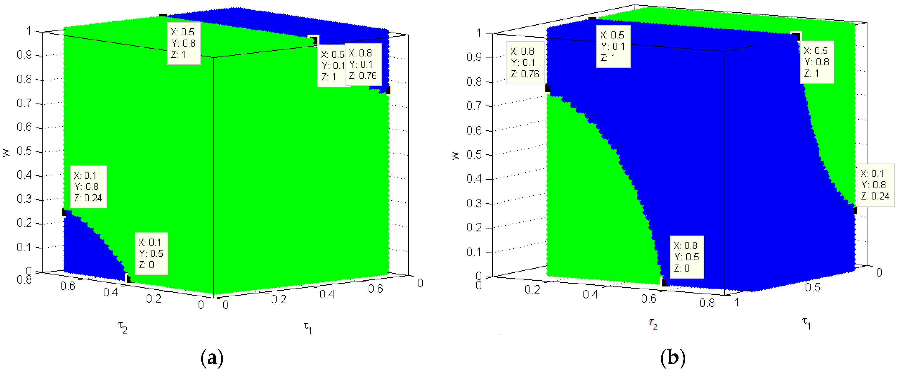
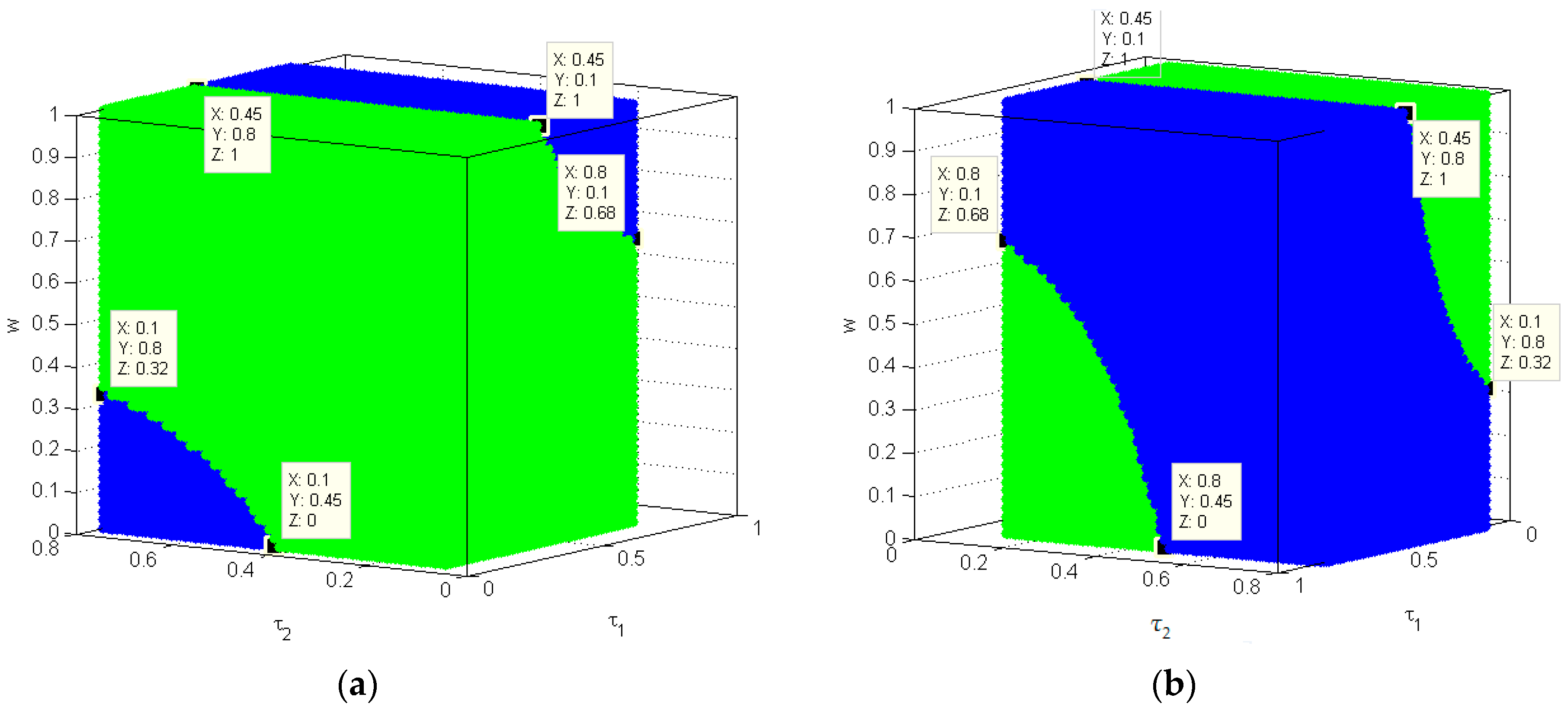
4.6. The Influence of ${\tau }_1$, ${\tau }_2$ and $w$ on the Stability of the Price $p_1$

In this section, we consider the influence of ${\tau }_1$, ${\tau }_2$ and $w$ on the stability of price $p_1$. Figure 12 and Figure 13 show that with the increase of ${\tau }_1$, $p_1$ is gradually moves to instability when ${\tau }_2>0.5$ and $w>0.24$. However, there is no obvious change to $p_1$ when ${\tau }_2<0.5$ and $w<0.76$. Similarly, when ${\tau }_1<0.5$ and $w<0.24$, $p_1$ moves from stable to unstable with ${\tau }_2$ becoming large. However, when ${\tau }_1>0.5$ and $w<0.76$, $p_1$ loses stability and results in a larger fluctuation with an increase in ${\tau }_2$. With ${\tau }_1<0.5$ and ${\tau }_2<0.5$ (green region in Figure 13), in this stable region, the change of $w$ have no effect on $p_1$. When ${\tau }_1<0.5$ and ${\tau }_2>0.5$, the increase of $w$ causes $p_1$ to shift from unstable to stable, and the value of $p_1$ becomes larger. When ${\tau }_1>0.5$ and ${\tau }_2<0.5$, $p_1$ shifts from a stable state to an unstable state with an increase of $w$, and $p_1$ generates a large fluctuation. As ${\tau }_1>0.5$ and ${\tau }_2>0.5$ (blue region in Figure 13), in this instability region, no matter how $w$ changes, $p_1$ is still unstable.

Figure 12. The influence of ${\tau }_1$, ${\tau }_2$ and $w$ on $p_1$. (a,b) are shown from different angles.

Figure 13. 3D parameter bifurcation in the (${\tau }_1$, ${\tau }_2$, $w$) plane, where different colors represent different regions of $p_1$: stability region (green), instability region (blue). (a,b) are shown from different angles. For interpretation of the references to color in this figure, the reader is referred to the web version of this article.

Through above analysis, in order to maintain the stability of $p_1$, the two firms must keep ${\tau }_1$ and ${\tau }_2$ in the green region (stability) of Figure 13. The boundary of the region is composed of the following points: A’(0.5, 0.8, 1), B’(0.1, 0.8, 0.24), C’(0.1, 0.5, 0), D’(0.8, 0.1, 0.76) and E’(0.5, 0.1, 1).

4.7. The Influence of ${\tau }_1$, ${\tau }_2$ and $w$ on the Profit ${\pi }_1$

In this part, we focus on the influence of ${\tau }_1$, ${\tau }_2$ and $w$ on the stability of profit ${\pi }_1$. We can see from Figure 14 and Figure 15 that when ${\tau }_2>0.45$ and $w>0.32$, the ${\pi }_1$ shifts gradually into instability with the increase of ${\tau }_1$. When ${\tau }_2<0.45$ and $w>0.68$, it shifts ${\pi }_1$ into an unstable state with ${\tau }_1$ becoming larger. Similarly, when ${\tau }_1<0.45$ and $w<0.32$, ${\pi }_1$ shifts from stable to unstable with ${\tau }_2$ increasing. However, when ${\tau }_1>0.45$ and $w<0.68$, ${\pi }_1$ loses stability and a larger fluctuation appears with an increase of ${\tau }_2$. As ${\tau }_1<0.45$ and ${\tau }_2<0.45$ (green region in Figure 15), the change of $w$ has no effect on ${\pi }_1$ in this stable region. When ${\tau }_1<0.45$ and ${\tau }_2>0.45$, ${\pi }_1$ shifts from an unstable state to a stable state with an increase of $w$, and the value of ${\pi }_1$ becomes larger. When ${\tau }_1>0.45$ and${\tau }_2<0.45$, ${\pi }_1$ shifts from the stable state, gradually becoming unstable with an increase of $w$, and ${\pi }_1$ appears to fluctuate greatly. As ${\tau }_1>0.45$ and ${\tau }_2>0.45$ (blue region in Figure 15), no matter how $w$ changes, ${\pi }_1$ is still unstable.

Figure 14. The influence of ${\tau }_1$, ${\tau }_2$ and $w$ on ${\pi }_1$. (a,b) are shown from different angles.

Figure 15. 3D parameter bifurcation in the (${\tau }_1$, ${\tau }_2$, $w$) plane, where different colors represent different regions of ${\pi }_1$: stability region (green), instability region (blue). (a,b) are shown from different angles. For interpretation of the references to color in this figure, the reader is referred to the web version of this article).

Through the above analysis, in order to maintain ${\pi }_1$ stability, the two firms must make ${\tau }_1$ and ${\tau }_2$ remain in the green region (stability) of Figure 15. The boundary of the region is composed of the following points: A’’(0.45, 0.8, 1), B’’(0.1, 0.8, 0.32), C’’(0.1, 0.45, 0), D’’(0.8, 0.1, 0.68) and E’’(0.45, 0.1, 1).

5. Chaos Control

We know that an unstable or chaotic market will cause price fluctuations and hurt firms’ bottom lines. Thus, we must take measures to control chaos. Therefore, some methods are found to control the chaos of the system, such as the OGY method (a control method of chaos was proposed by Ott E., Grebogi C. and Yorke J.A. in America) [20], modified straight-line stabilization method [21], time-delayed feedback method [22], pole placement method [23], and so on. In this section, we use the state variables’ feedback and parameter variation to control the chaotic system (21) [24]. The controlled system is given by:

$$\{\begin{array}{l}\stackrel{·}{p_1}(t)=(1-\mu ){\nu }_1{p}_1(a_1-2b_{1}w{p}_1(t-{\tau }_1)-2b_1(1-w)p_1(t-{\tau }_2)+d_1{p}_2+b_1{c}_1)+\mu p_1\\ \stackrel{·}{p_2}(t)=(1-\mu ){\nu }_2{p}_2(a_2-2b_2{p}_2+d_{2}w{p}_1(t-{\tau }_1)+d_2(1-w)p_1(t-{\tau }_2)+b_2{c}_2)+\mu p_2\end{array}$$

(22)

In order to show more clearly the effect of chaos control, we only let ${\tau }_1=0.4$, ${\tau }_2=0.8$, while other parameter values remain unchanged. We know that $({\tau }_1,{\tau }_2)=(0.4,0.8)$ in the blue region of Figure 9, and Equation (21) is chaotic. Without chaos control, the dynamic properties of the system (21) are shown in Figure 16.

Figure 16. The Equation (21) is unstable when $({\tau }_1,{\tau }_2)=(0.4,0.8)$. (a) Power spectrum; (b) Attractor.

Figure 17 shows that the bifurcation point of Equation (22) is $\mu =0.3819$. When $\mu <0.3819$, Equation (22) is chaotic, and when $\mu >0.3819$, Equation (22) is stable. The largest Lyapunov exponent plot verifies the correctness of the conclusion.

Figure 17. The influence of $\mu$ on the stability of the Equation (22) when $({\tau }_1,{\tau }_2)=(0.4,0.8)$. (a) Bifurcation diagram; (b) The largest Lyapunov exponent plot.

First, let $\mu =0.3<0.3819$, the power spectrum and attractor of Equation (22) are as shown in Figure 18. We find that Equation (22) is still in the state of chaos, which is not effectively controlled. Secondly, let $\mu =0.45>0.3819$, the power spectrum and attractor of Equation (22) are as shown in Figure 19. It clearly shows that Equation (22) gets out of chaos and becomes stable. Thus, chaos control is successful when the control parameter $\mu$ is sufficiently large.

Figure 18. The Equation (22) is unstable when $\mu =0.3<0.3819$ for $({\tau }_1,{\tau }_2)=(0.4,0.8)$. (a) Power spectrum; (b) Attractor.

Figure 19. The Equation (22) is stable when $\mu =0.45>0.3819$ for $({\tau }_1,{\tau }_2)=(0.4,0.8)$. (a) Power spectrum; (b) Attractor.

6. Conclusions

This paper establishes a continuous Bertrand duopoly game model with two-stage delay. We choose the delay and weight as the research parameters, and focus on the influence of parameters on the dynamic characteristics of the system, such as bifurcation, chaos, and initial value sensitivity, etc. We study the influence of parameters on the system from four aspects. Firstly, we consider ${\tau }_2$ as a parameter when ${\tau }_1=0$. Our research focus is the influence of ${\tau }_2$ on the stability of the system. Secondly, ${\tau }_2$ as a constant, we study the influence of ${\tau }_1$ on the stability of the system through the power spectrum, attractor, bifurcation diagram, and LLE plot. Thirdly, we focus on the effect of ${\tau }_1$ and ${\tau }_2$ on the stability of the system by the 2D parameter bifurcation diagram, 3D surface chart, and stability region. Finally, we consider the influence of delay and weight on the stability of the system through the 4D cubic chart and 3D parameter bifurcation diagram. The stability region of the system is given. At the end of this paper, the effective control of chaos is carried out by a control strategy of the state variables’ feedback and parameter variation. It is successful to avoid the destruction of chaos for the economic system.

This study shows that the change of delay will lead to the system from stable state to unstable state, which causes a large fluctuation in prices and results in a decline in profits. The above analysis can provide help a firm’s decision-making process to avoid pushing the price into chaos.

References

- Brianzoni, S.; Luca, G.B.; Michetti, E. Dynamics of a Bertrand duopoly with differentiated products and nonlinear costs: Analysis, comparisons and new evidences. Chaos Solitons Fractals 2015, 79, 191–203. [Google Scholar] [CrossRef]
- Ahmed, E.; Elsadany, A.A.; Tonu, P. On Bertrand duopoly game with differentiated goods. Appl. Math. Comput. 2015, 251, 169–179. [Google Scholar] [CrossRef]
- Zhao, L.; Zhang, J. Analysis of a duopoly game with heterogeneous players participating in carbon emission trading. Nonlinear Anal. Model. Control 2014, 19, 118–131. [Google Scholar]
- Ma, J.; Guo, Z. The influence of information on the stability of a dynamic Bertrand game. Commun. Nonlinear Sci. Numer. Simul. 2016, 30, 32–44. [Google Scholar] [CrossRef]
- Fanti, L.; Gori, L.; Mammana, C.; Michetti, E. Local and global dynamics in a duopoly with price competition and market share delegation. Chaos Solitons Fractals 2014, 69, 253–270. [Google Scholar] [CrossRef]
- Yi, Q.G.; Zeng, X.J. Complex dynamics and chaos control of duopoly Bertrand model in Chinese air-conditioning market. Chaos Solitons Fractals 2015, 76, 231–237. [Google Scholar] [CrossRef]
- Ma, J.; Xie, L. Study on the complexity pricing game and coordination of the duopoly air conditioner market with disturbance demand. Commun. Nonlinear Sci. Numer. Simul. 2016, 32, 99–113. [Google Scholar] [CrossRef]
- Agiza, H.N.; Hegazi, A.S.; Elsadany, A.A. Complex dynamics and synchronization of duopoly game with bounded rationality. Math. Comput. Simul. 2002, 58, 133–146. [Google Scholar] [CrossRef]
- Yali, L. Dynamics of a delayed Duopoly game with increasing marginal costs and bounded rationality strategy. Procedia Eng. 2011, 15, 4392–4396. [Google Scholar] [CrossRef]
- Zhang, J.; Wang, G. Complex Dynamics of Bertrand duopoly games with bounded rationality. World Acad. Sci. Eng. Technol. 2013, 79, 106–110. [Google Scholar]
- Li, T.; Ma, J. Complexity analysis of the dual-channel supply chain model with delay decision. Nonlinear Dyn. 2014, 78, 2617–2626. [Google Scholar] [CrossRef]
- Ma, J.; Guo, Z. The parameter basin and complex of dynamic game with estimation and two-stage consideration. Appl. Math. Comput. 2014, 248, 131–142. [Google Scholar] [CrossRef]
- Elabbasy, E.M.; Agiza, H.N.; Elsadany, A.A. Analysis of nonlinear triopoly game with heterogeneous players. Comput. Math. Appl. 2009, 57, 488–499. [Google Scholar] [CrossRef]
- Peng, J.; Miao, Z.H.; Peng, F. Study on a 3-dimensional game model with delayed bounded rationality. Appl. Math. Comput. 2011, 218, 1568–1576. [Google Scholar] [CrossRef]
- Agiza, H.N.; Elsadany, A.A.; El-Dessoky, M.M. On a new Cournot duopoly game. J. Chaos 2013, 2013, 487803. [Google Scholar] [CrossRef]
- Li, Q.; Ma, J. Research on price Stackelberg game model with probabilistic selling based on complex system theory. Commun. Nonlinear Sci. Numer. Simul. 2016, 30, 387–400. [Google Scholar] [CrossRef]
- Zhang, J.-F. Bifurcation analysis of a modified Holling–Tanner predator–prey model with time delay. Appl. Math. Model. 2012, 36, 1219–1231. [Google Scholar] [CrossRef]
- Hale, J.K. Theory of Functional Differential Equations; Springer: New York, NY, USA, 1977. [Google Scholar]
- Gori, L.; Guerrini, L.; Sodini, M. Hopf bifurcation and stability crossing curves in a cobweb model with heterogeneous producers and time delays. Nonlinear Anal. Hybrid Syst. 2015, 18, 117–133. [Google Scholar] [CrossRef]
- Agiza, H.N. On the Analysis of stability, Bifurcations, Chaos and Chaos Control of Kopel Map. Chaos Solitons Fractals 1999, 10, 1909–1916. [Google Scholar] [CrossRef]
- Du, J.; Huang, T.; Sheng, Z. Analysis of decision-making in economic chaos control. Nonlinear Anal. Real World Appl. 2009, 10, 2493–2501. [Google Scholar] [CrossRef]
- Holyst, J.; Urbanowicz, K. Chaos control in economic model by time-delayed feedback method. Phys. A Stat. Mech. Appl. 2000, 287, 587–598. [Google Scholar] [CrossRef]
- Matsumoto, A. Controlling the Cournot–Nash chaos. J. Optim. Theory Appl. 2006, 128, 379–392. [Google Scholar] [CrossRef]
- Luo, X.S.; Chen, G.R.; Wang, B.H.; Fang, J.Q.; Zou, Y.L.; Quan, H.J. Control of period-doubling bifurcation and chaos in a discrete nonlinear system by the feedbackof states and parameter adjustment. Acta Phys. Sin. 2003, 52, 790–794. [Google Scholar]
© 2016 by the authors; licensee MDPI, Basel, Switzerland. This article is an open access article distributed under the terms and conditions of the Creative Commons Attribution (CC-BY) license (http://creativecommons.org/licenses/by/4.0/).