Structures in Sound: Analysis of Classical Music Using the Information Length

Abstract

We show that music is represented by fluctuations away from the minimum path through statistical space. Our key idea is to envision music as the evolution of a non-equilibrium system and to construct probability distribution functions (PDFs) from musical instrument digital interface (MIDI) files of classical compositions. Classical music is then viewed through the lens of generalized position and velocity, based on the Fisher metric. Through these statistical tools we discuss a way to quantitatively discriminate between music and noise.

1. Introduction

Music plays an intricate part of human life. As a result there is a large body of work devoted to the analysis of music. Going back to the Greeks, “Pythagoras was the first to discover the fundamental connection between mathematics and music” [1]. Since then countless works have been published revealing the structure of music through mathematical language, e.g., see [2,3,4,5]. The application of information theory has also been applied to music often with the goal of equating a measure of uncertainty inherent in the Shannon information with uncertainty in a musical composition [6,7,8,9].

Of particular interest here are the various power laws that have been found in different measures of music. In particular, Voss and Clarke [10] examined the output voltage of sound recordings and found that different aspects of recordings followed power laws. For example, the loudness of music and speech follows a power law but the voltage (time signal itself) does not. Power laws have been found in music using both continuous signals such as Voss and Clarke or Serrà et al. [11], or through digitized music [12,13,14]. Here we show that using digitized music, through musical instrument digital interface (MIDI) files, classical compositions also follow approximate power laws in a statistical space, despite mathematically having a time dependent exponent.

The concept of a minimum path, or geodesic through a given space is found in many branches of physics [15,16,17,18]. Music may be included in this list by its deviation from the minimum path in statistical space. This is manifested by power laws which are generated through the periodic forcing in statistical space.

Here we refer to the information gained from observing state x knowing the distribution $p\left(x\right)$ by $I=-logp\left(x\right)$ [19]. The information variation is then produced from the temporal change in probability distribution functions (PDFs) and is utilized in this work to quantify the generalized fluctuating energy and velocity associated with information variation in a metric space parametrized by time. The total distance traveled in this metric space represents total accumulative information transfer in time and is quantified by information length $\mathcal{L}$. Similarly, the action $\mathcal{J}$ of the music is computed from the time integral of the energy of the music by using the square of the velocity as energy. These measures are simply the generalizations of the thermodynamic length originally developed by Weinhold [20] and Rupiener [21] and first extended out of equilibrium by Salamon and Berry [22]. By focusing on several compositions to highlight our results, we will show that: (i) both $\mathcal{L}$ and $\mathcal{J}$ increase with time T as a power law, its index approaching unity in time for almost all compositions; (ii) $\mathcal{J}-{\mathcal{L}}^2/T$ exhibits a power law $\propto T^{1+m}$, where m signifies the deviation from the minimum path; (iii) By comparing musical compositions with results obtained from Gaussian white and colored noise, we show that music experiences the analogue of periodic forcing in statistical space while noise does not. This periodic forcing is manifested through the change in velocity in statistical space, the variance of which is exactly the term which accounts for the deviation from the minimum path. Meaning noise can be quantitatively differentiated from music through velocity in statistical space. These results highlight the organization of music into “regularity” (an almost constant information flow) and deviations away from this constant flow. The remainder of this paper is organized as follows: Section 2 introduces $\mathcal{L}$ and $\mathcal{J}$. Section 3 presents how PDFs are constructed from MIDI files. Our results are presented in Section 4 and conclusions are in Section 5.

2. Information Variation ($\mathcal{L}$ and $\mathcal{J}$)

In understanding the evolution of a non-equilibrium system, a key physical quantity is the temporal variation in the PDF of state x, i.e., $p(x,t)$, where x belongs to the state space Ω. The information gained from observing state $p(x,t)$ can be measured through the information measure, $-logp(x,t)$ [23]. Due to the conservation of probability,

$$-{\int }_{\Omega }dxp(x,t)\frac{\partial logp(x,t)}{\partial t}=0.$$

(1)

Thus the first moment of the information is always zero. The second moment, which is equivalent to $\langle -\frac{{\partial }^{2}logp(x,t)}{\partial t^2}\rangle$, is not zero. This means we quantify the variation in information through the second moment as (c.f. [24]) defined through the Fisher metric

$$\begin{array}{cc}\hfill \mathcal{L}& ={\int }_0^{T}dt\sqrt{\int dx\frac{1}{p(x,t)}{\left(\frac{\partial p(x,t)}{\partial t}\right)}^2}\hfill \\ & =2{\int }_0^{T}dt\sqrt{\int dx{\left(\frac{\partial q(x,t)}{\partial t}\right)}^2}\hfill \\ & ={\int }_0^{T}v\left(t\right)dt=\int d\mathcal{L}.\hfill \end{array}$$

(2)

Thus

$$v\left(t\right)=2\sqrt{\int dx{\left(\frac{\partial q(x,t)}{\partial t}\right)}^2},$$

(3)

represents the effective velocity through statistical space from $t=0$, to $t=T$, while $\mathcal{E}\left(t\right)=v{\left(t\right)}^2$ is the associated energy given by the square of this velocity [22]. The second line follows from replacing $p(x,t)=q{(x,t)}^2$ (see [29]), which is needed to avoid un-physical values when $p(x,t)=0$ for some x and t (as the system may have explored only a small portion of its state space). For the discrete non-equilibrium case see [30] and for applications in Quantum Mechanics, see [29] and [31]. In the case where control parameters ${\lambda }^i$’s ($i=1,2,3,...$) of a system are known as a function of time (e.g., near equilibrium), Equation (2) can be recast in the form of the metric tensor $g_{ij}$ (see, e.g., [25,26,27])

$$g_{ij}=\int dxp(x,\lambda \left(t\right))\frac{\partial logp(x,\lambda (t\left)\right)}{\partial {\lambda }^i}\frac{\partial logp(x,\lambda (t\left)\right)}{\partial {\lambda }^j},$$

(4)

as

$$\mathcal{E}\left(t\right)=v{\left(t\right)}^2=\sum _{i,j}\frac{d{\lambda }^i}{dt}{g}_{ij}\frac{d{\lambda }^j}{dt}.$$

(5)

$g_{ij}$ in Equation (5) is the metric tensor that gives the Riemannian metric [28] in the parameter space λ’s. Since often the control parameters of a system are not known, it is much more convenient to use Equation (2) directly in terms of PDFs. In terms of $\mathcal{E}\left(t\right)$, we measure the total accumulated energy between $t=0$ and $t=T$ by the information action $\mathcal{J}$,

$$\mathcal{J}={\int }_0^{T}dt\mathcal{E}\left(t\right)={\int }_0^{T}dtv{\left(t\right)}^2.$$

(6)

We note that the distance $\mathcal{L}$ is dimensionless while $\mathcal{J}$ has the dimension of the inverse time. Equations (2) and (6) quantify the accumulative information variation and are analogous to the relations for the distance and the action for a particle with unit mass in classical mechanics, which will be expanded on in Section 4.2. For the analysis of classical music, we will use discrete approximations of Equations (2) and (6),

$$\begin{array}{ccc}\hfill \mathcal{L}& =& 2\sum _{i=2}^N\Delta t\sqrt{\sum _x{\left(\frac{\Delta q_i}{\Delta t}\right)}^2},\hfill \end{array}$$

(7)

$$\begin{array}{ccc}\hfill \mathcal{J}& =& 4\sum _{i=2}^N\Delta t\sum _x{\left(\frac{\Delta q_i}{\Delta t}\right)}^2.\hfill \end{array}$$

(8)

Whether we are talking about the discrete or continuous versions of $\mathcal{L}$ and $\mathcal{J}$ are being used will be clear from the context. To highlight the relationship between $\mathcal{J}$ and $\mathcal{L}$, we use $u=1$ in the following Cauchy–Schwartz inequality

$${\int }_0^T\mathcal{E}\left(t\right)dt{\int }_0^T{u}^{2}dt\ge {\left({\int }_0^{T}v\left(t\right)udt\right)}^2,$$

(9)

which gives the well known result, $\mathcal{J}\ge {\mathcal{L}}^2/T$. Note that the minimum value of $\mathcal{J}-{\mathcal{L}}^2/T$ would be achieved for geodesics in statistical space. This minimum value, $\mathcal{J}={\mathcal{L}}^2/T$ is achieved only when $v\left(t\right)$ is constant [32] in Equations (2) and (6). In the case of constant $v\left(t\right)$, the evolution of the system can be viewed as a “free” motion. To quantify the difference between $\mathcal{J}$ and ${\mathcal{L}}^2/T$, it is useful to consider the time average of $v\left(t\right)$ and $\mathcal{E}\left(t\right)$ [33] as follows:

$${\langle v\left(t\right)\rangle }_T=\frac{1}{T}{\int }_0^{T}dtv\left(t\right),{\langle \mathcal{E}\left(t\right)\rangle }_T=\frac{1}{T}{\int }_0^{T}dt\mathcal{E}\left(t\right).$$

(10)

This lets us write a time averaged variance of the velocity,

$$\begin{array}{cc}\hfill V_T& ={\langle v{\left(t\right)}^2\rangle }_T-{\langle v\left(t\right)\rangle }_T^2,\hfill \\ & ={\langle \mathcal{E}\left(t\right)\rangle }_T-{\langle v\left(t\right)\rangle }_T^2.\hfill \end{array}$$

(11)

Relating Equation (11) to Equations (2) and (6),

$$\begin{array}{ccc}\hfill \mathcal{J}-\frac{{\mathcal{L}}^2}{T}& =& T\left({\langle \mathcal{E}\left(t\right)\rangle }_T-{\langle v\left(t\right)\rangle }_T^2\right),\hfill \\ & \approx & T^{1+m},\hfill \end{array}$$

(12)

where typically $m\ll 1$. the deviation away from the minimum path is given by fluctuations in the time averaged velocity. Alternatively, put another way, the time averaged variance of the system is related to the distance it travels.

Equation (11) also allows us to understand the evolution of $\mathcal{J}$ and $\mathcal{L}$ in relation to one another for the evolution of a musical composition. One may expect for example that $T^{1+m}\to T$, if m decreases in time. While this is true, it is not the complete story. Upon closer examination of the velocity in Section 4.2 we will see that the key characteristic between music, and noise, is that music experiences periodic forcing while noise experiences a continuous distribution of forcing. The detailed analysis on $\mathcal{L}$, $\mathcal{J}$ and $\mathcal{J}/T-{(\mathcal{L}/T)}^2$ for famous classical compositions are presented in Section 4.

3. Music as a Non-Equilibrium System

To frame music in the context of generalized distances and energies we envision a composition (such as Vivaldi’s Concerto Summer) as a non-equilibrium system where each note represents a state x of the system. As a piece of music evolves, each instrument transitions between states, while the simultaneous occupation of a set of states by all instruments in a single time step creates the sound we hear. In western music, the musical scale is often divided into 11 octaves where each note belonging to an octave has a $2:1$ or $1:2$ relationship between its frequency and the frequency of the corresponding note in the octave below or above it. Octaves are then made up of semitones or half notes. These semitones will be used as the states of the system. The states a composition occupies are used to construct the probability over all instruments $p(x,t)$ of a note being played in a coarse grained time interval, $\Delta t$. The time dependence of $p(x,t)$ creates the variation in information.

In defining the state x of a note belonging to $p(x,t)$, we utilise MIDI files as they contain detailed information about the composition. Specifically, the MIDI file format represents a piece of sheet music as a series of numbers that are used by a computer in recreating a given composition (each MIDI file used here is freely available at [34]). Each note from octave 0 to octave 10 is given a MIDI number. Using a MIDI file our state space is then characterized by 129 states. States 0 to 127 correspond to each possible note while the state 128 represents a rest (i.e., no note being played). These MIDI numbers and their corresponding notes are shown in

Table 1. Each MIDI number corresponds to an octave listed in the left column and a note, listed on the top row (# indicates sharps).

Octave	Notes
Number	C	C#	D	D#	E	F	F#	G	G#	A	A#	B
0	0	1	2	3	4	5	6	7	8	9	10	11
1	12	13	14	15	16	17	18	19	20	21	22	23
2	24	25	26	27	28	29	30	31	32	33	34	35
3	36	37	38	39	40	41	42	43	44	45	46	47
4	48	49	50	51	52	53	54	55	56	57	58	59
5	60	61	62	63	64	65	66	67	68	69	70	71
6	72	73	74	75	76	77	78	79	80	81	82	83
7	84	85	86	87	88	89	90	91	92	93	94	95
8	96	97	98	99	100	101	102	103	104	105	106	107
9	108	109	110	111	112	113	114	115	116	117	118	119
10	120	121	122	123	124	125	126	127	–	–	–	–

.

The “tick” is the time unit used by the MIDI format. One tick is equivalent to a certain number of milliseconds, specified in the header of each MIDI file. In this work we use $\Delta t=\frac{seconds}{tick}$ as specified in the header. These are all on the order of $\Delta t\approx 1\times {10}^{-3}$ s. However it should be noted the choice of $\Delta t$ is a free parameter and is the coarse graining scale of the system. The limiting factor is the size of errors one desires between $∥\frac{1}{p(x,t)}\frac{\Delta p(x,t)}{\Delta t}-4\frac{\Delta q(x,t)}{\Delta t}∥$ where $\parallel ·\parallel$ is some norm and $\Delta p=p(x,i\Delta t)-p(x,(i-1)\Delta t)$, $\Delta q=q(x,i\Delta t)-q(x,(i-1)\Delta t)$. For all subsequent analysis we use the discrete version of $\mathcal{L}$ and $\mathcal{J}$, Equations (7) and (8).

To then generate a PDF, we measure the number of occurrences of each MIDI number over all instruments for one time step of a given composition. Normalizing this frequentist approach at each time step, generates a sequence of discrete PDFs which can be analysed using Equations (7) and (8).

To compare our results for music, we will also calculate $\mathcal{L}$ and $\mathcal{J}$ from Gaussian white and “colored” noise. The white noise signal $z\left(t\right)$, $0\le t\le T$ will have mean, $\langle z\left(t\right)\rangle =0$ and variance, $\langle z\left(t\right)z\left(t^{\prime }\right)\rangle =D\delta (t-t^{\prime })$, where D is the noise intensity [35]. The colored noise will be a realization of an Ornstein–Uhlenbeck [36] process with finite correlation time τ, through the algorithm due to Bartosch [37]. A realization is characterized through the mean and variance, $\langle x\left(t\right)\rangle =0$ and $\langle x\left(t\right)x\left(t^{\prime }\right)\rangle ={\sigma }^2{e}^{-|t^{\prime }-t|/\tau }$ respectively.

Since we want to compare this to MIDI files which are made up from 129 disjoint states, the minimum and maximum of a realization of noise is broken up into 129 equal states $B_i$, $i=1,2,\cdots ,129$. $B_1$ corresponds to note 0 and $B_{128}$ is note 127 while $B_{129}$ represents a rest. Thus, from a signal of a given length, we can calculate $p(x,t)$ just as we do for musical compositions. In the white noise example we use Vivaldi’s Summer as our reference by generating noise signals of equal length and using the time step $\Delta t$ from this composition.

4. Results

We compute PDFs and analyse a collection of famous classical compositions with four being shown in greater detail. These compositions are typical examples from the overall collection, the rest of which are shown in the Supplementary Materials. These “selected” compositions are Vivaldi’s Summer, Beethoven’s Ninth Symphony 2nd movement, Mozart’s violin Concerto No. 3, and Tchaikovsky’s 1812 Overture. Every composition will be seen to follow an approximate power law with periodic forcing. What makes this particularly interesting is that each PDF that generates these simple relationships is strongly intermittent as can be seen in a typical example of $p(x,t)$, see in Figure S1.

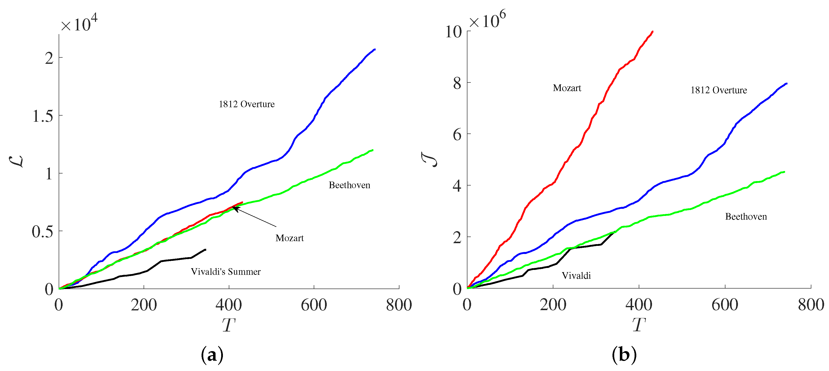
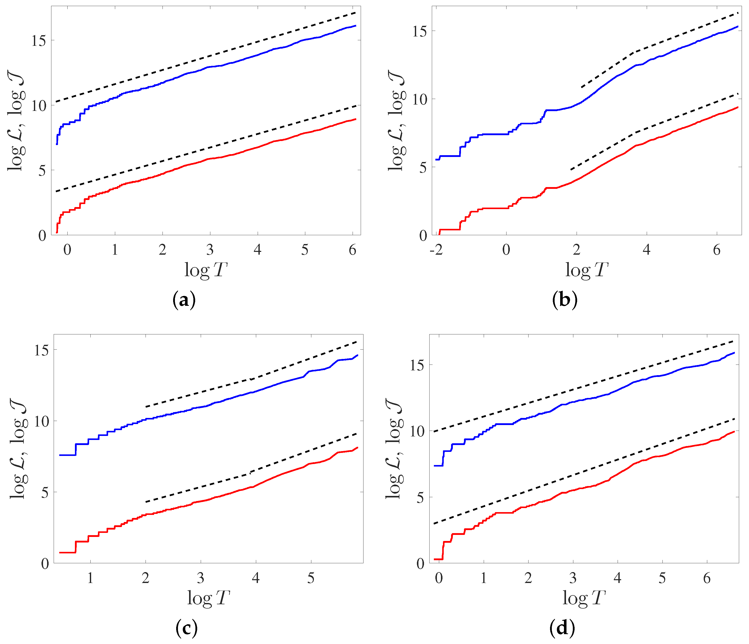
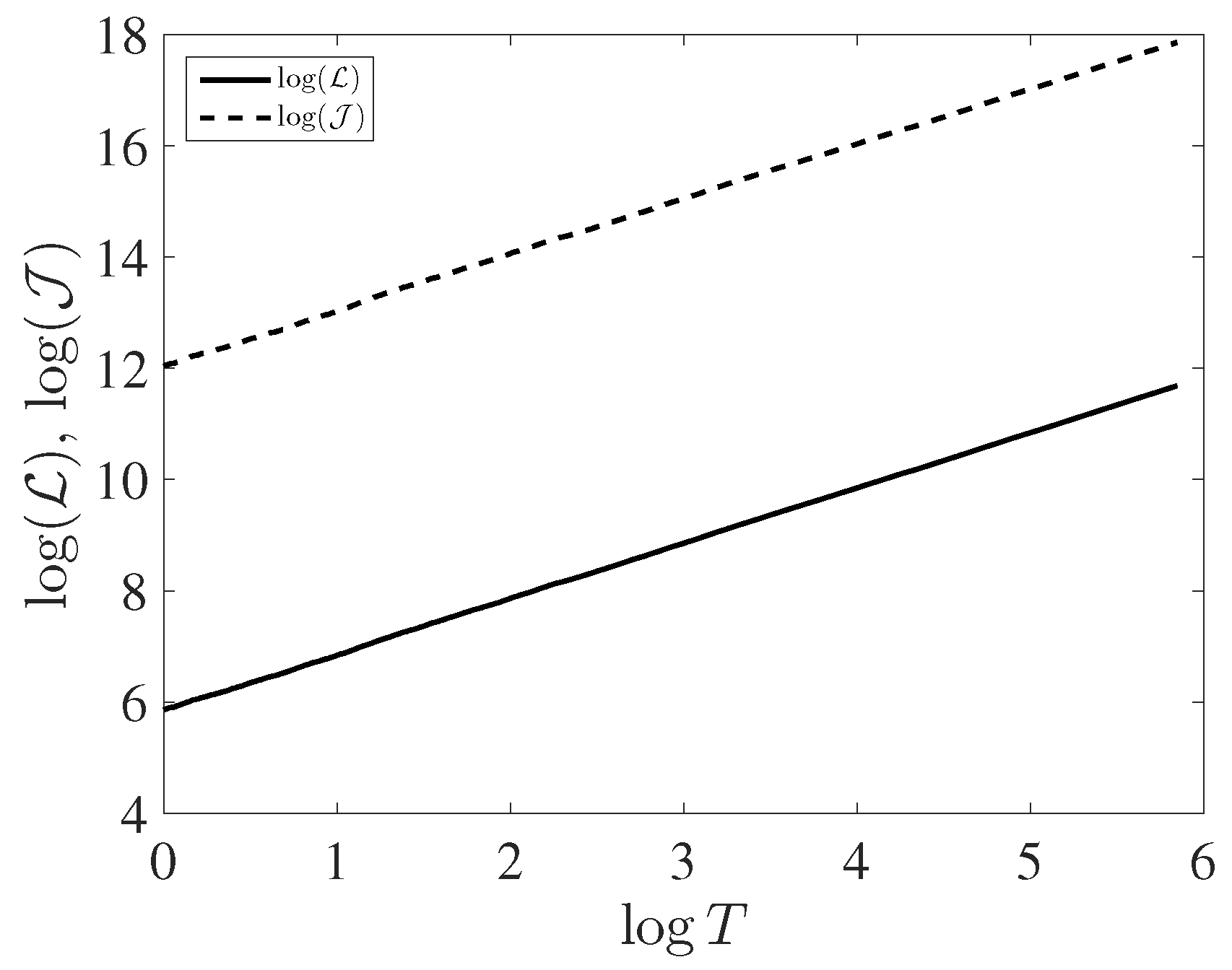
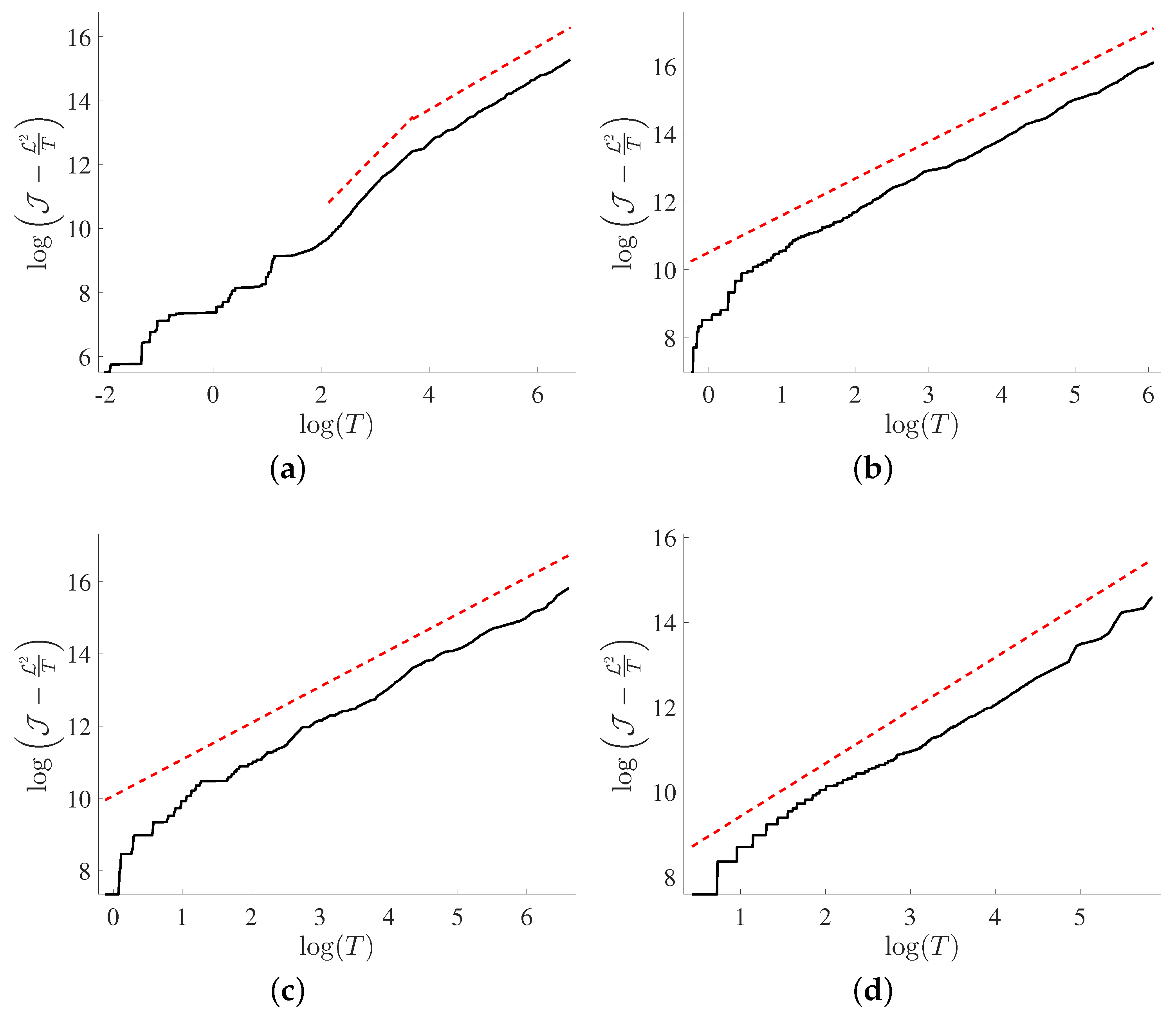
4.1. Power Law Scalings

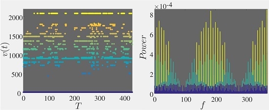
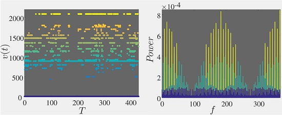
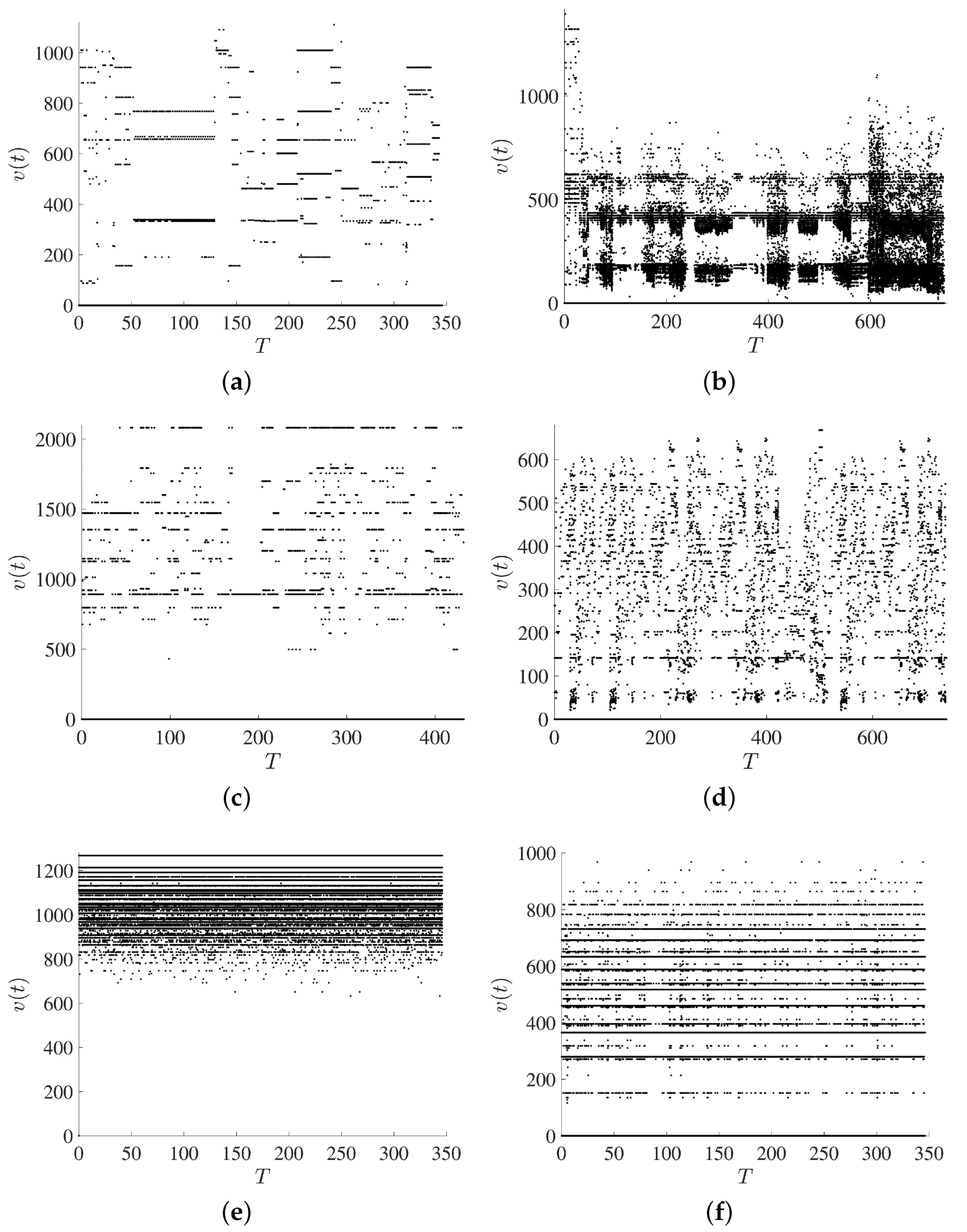
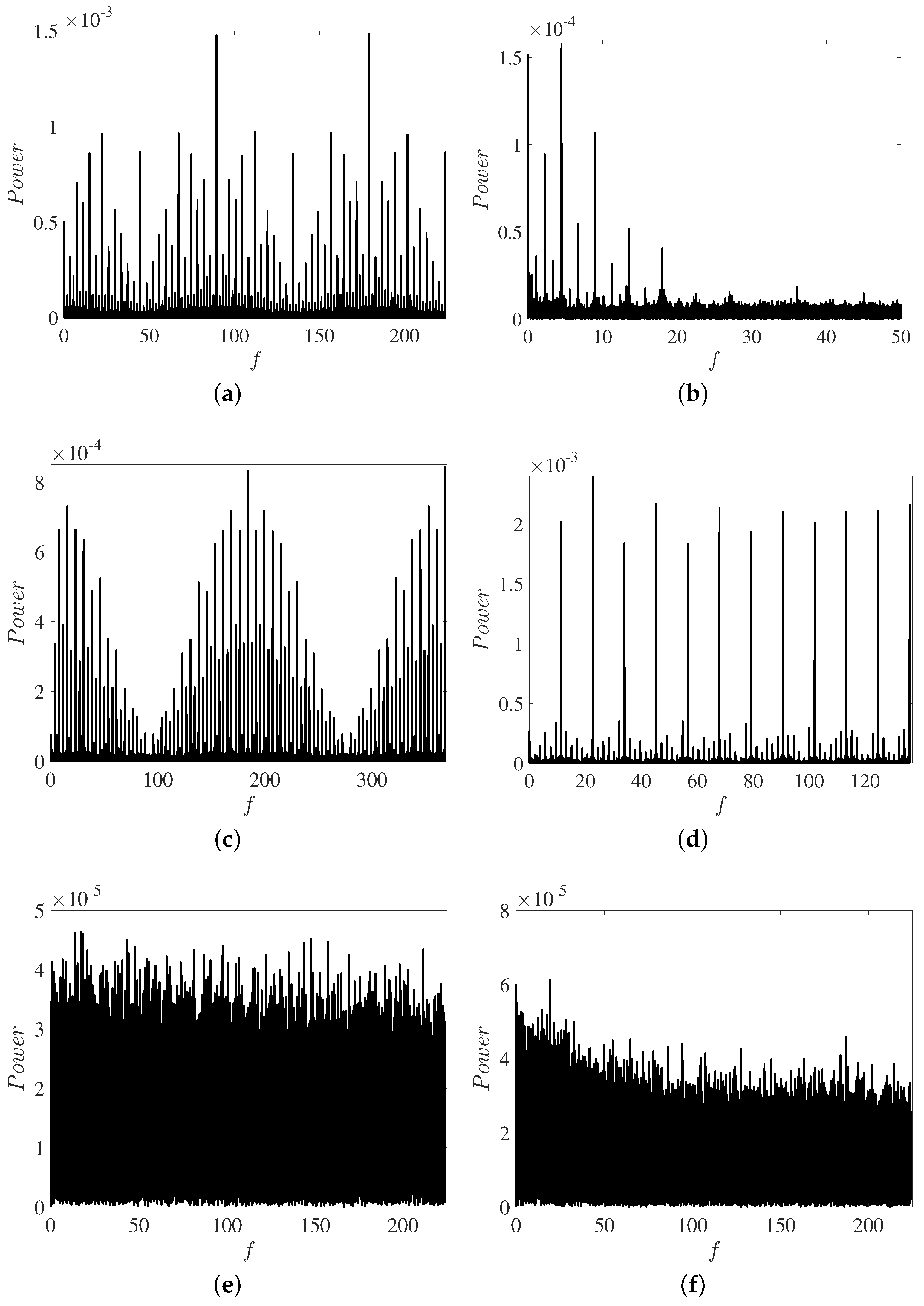
Using the PDFs generated from four typical compositions we calculate $\mathcal{L}$ and $\mathcal{J}$ as a function of time and plot them in Figure 1.

Detailed features can be seen in Figure 2 which shows results for different compositions separately in log–log scales. log–log scaling for the rest of the compositions can be seen in Figure S2. Power law indices of $\mathcal{L}$ and $\mathcal{J}$ are thus determined by linear fitting, as shown using dashed lines and are summarized along with all the other compositions in

Table 2. Coefficients $c_{\mathcal{L}}$, $c_{\mathcal{J}}$, exponents $M_{\mathcal{L}}$ and $M_{\mathcal{J}}$ for all compositions along with the corresponding $R^2$ values. Every composition except Brahms’ string quartet and Vivaldi’s Summer are near one, or evolve to an exponent around one. This signifies a constant flow of information.

T0 (s)	Composition			log $ℒ$		log $𝒥$
		c$ℒ$	M$ℒ$	R2	c$𝒥$	M$𝒥$	R2
0.784	Mozart’s violin Concerto No. 3	2.61	1.043	0.998	$1.37\times {10}^3$	1.088	0.996
7.39	Vivaldi’s Summer	3.30	1.054	0.996	$2.73\times {10}^3$	$1.033$	$0.991$
$49.4$		$0.9562$	$1.399$	$0.991$	$0.644\times {10}^3$	$1.388$	$0.981$
$8.46$	Beethoven’s 9th Symphony 2nd movement	$1.09$	$1.476$	$0.999$	$0.472\times {10}^3$	$1.724$	$0.996$
$40.37$		$2.9134$	$0.980$	$0.999$	$6.91\times {10}^3$	$0.981$	$0.999$
$0.889$	Tchaikovsky’s 1812 Overture	$8.37$	$1.177$	$0.987$	$8.61\times {10}^3$	$1.018$	$0.991$
$0.460$	Mozart piano Concerto No. 3	$12.4$	$1.136$	$0.992$	$4.81\times {10}^3$	$1.159$	$0.993$
$0.640$	Brahms’ string quartet Op.51	$2.02$	$1.240$	$0.989$	$609.63$	$1.257$	$0.985$
$0.286$	Bach Brandenburg Concerto No. 3 1st movement	$6.77$	$0.990$	$0.999$	$1.83\times {10}^3$	$0.969$	$0.997$
$2.72$	Bach Brandenburg Concerto No. 3 2nd movement	$3.77$	$1.245$	$0.996$	$0.597\times {10}^3$	$1.48$	$0.993$
$33.11$		$9.26$	$0.964$	$0.999$	$2.54\times {10}^3$	$0.95$	$0.999$
$0.368$	Liszt Ballade No. 2	$7.16$	$1.000$	$0.996$	$2.38\times {10}^3$	$0.999$	$0.998$
$0.8702$	Chopin Ballade in F Minor, Op. 52	$9.72$	$1.049$	$0.987$	$4.71\times {10}^3$	$1.05$	$0.986$
$1.002$	White noise	$1.11\times {10}^3$	$1.00$	$1.00$	$1.25\times {10}^6$	$1.00$	$1.00$
$1.002$	correlated noise, $\tau =20$	$505.7$	$1.00$	$1.00$	$2.9\times {10}^5$	$1.00$	$1.00$
$1.002$	correlated noise, $\tau =112$	$354.73$	$0.994$	$1.00$	$1.78\times {10}^5$	$0.989$	$1.00$

. The quality of a linear fit is measured using the standard R-squared value. All R-squared values in Table 2 are close to one, meaning power laws are very good approximations to $\mathcal{J}$ and $\mathcal{L}$.

All compositions after an initial transient phase follow power law relations as we expect from Equation (11). Furthermore, $\mathcal{L}$ and $\mathcal{J}$ for every composition other than Vivaldi’s Summer and Brahms’ string quartet evolve to become approximately $M_{\mathcal{L}}\approx M_{\mathcal{J}}\approx 1$. Where $M_{\mathcal{L}}=M_{\mathcal{J}}=1$ means there is a constant rate of information change, as the system evolves. The constant flow of information and energy is equivalent to the system taking the minimum path through statistical space [32]. Vivaldi and Brahms are exceptions with slopes for $\mathcal{L}$ and $\mathcal{J}$ that are farther from one.

To compare the power law behaviour of music to noise, Figure 3 shows the log–log plot of $\mathcal{L}$ and $\mathcal{J}$ for a realization of noise, There is again a power law relation, though this is almost exactly linear in time. Starting around one second, each realization follows the same minimum through statistical space.

Since both $\mathcal{L}$ and $\mathcal{J}$ follow power law relations,

$$\mathcal{L}=c_{\mathcal{L}}{T}^{M_{\mathcal{L}}},\mathcal{J}=c_{\mathcal{J}}{T}^{M_{\mathcal{J}}}.$$

(13)

For short correlated noise $M_{\mathcal{L}}=M_{\mathcal{J}}=1$ meaning $\mathcal{J}-{\mathcal{L}}^2/T$ takes on a simple form,

$$\mathcal{J}-{\mathcal{L}}^2/T\approx T\left(c_{\mathcal{J}}-c_{\mathcal{L}}^2\right)=0.$$

(14)

We check that $c_{\mathcal{J}}-c_{\mathcal{L}}^2\sim 0$, as can be seen in Table 2. In contrast, the values of $c_{\mathcal{J}}$ and $c_{\mathcal{L}}$ for music significantly deviate from zero (see Table 2). The deviation of $\mathcal{L}$ and $\mathcal{J}$ in time from an exact linear increase is then proposed as a defining characteristic of music. Taking a closer look at $\mathcal{J}-{\mathcal{L}}^2/T$ the same data as Figure 1 is used for Figure 4. Specifically, Figure 4 shows the log–log plots of $\mathcal{J}-{\mathcal{L}}^2/T$ in black, from the initial time where $\mathcal{J}\ne {\mathcal{L}}^2/T$. Each composition has three main phases of its evolution, initially following the minimum path $\mathcal{J}={\mathcal{L}}^2/T$. This is often caused by single notes being played at the beginning of compositions. Next there is an initial transient phase where $\mathcal{J}-{\mathcal{L}}^2/T$ undergoes large fluctuations before the system settles into its power law behaviour. The third phase is when again to a very good approximation there is a balance between the cumulative kinetic energy used and the distance traveled through statistical space as measured by $\mathcal{J}-{\mathcal{L}}^2/T$. Each least squares fit is shown with dashed red lines, and the initial time $T_0$ of each fitting is shown in

Table 3. $T_0$ is the initial time for the fitting of $log\left(\mathcal{J}-{\mathcal{L}}^2/T\right)$ shown with red dashed lines for the selected pieces. m is the exponent minus one, which are all small towards the end of the evolutions. $R^2$ shows that each linear fits are good approximation to the function.

Composer	T0 (s)	m	R2
Beethoven’s Symphony No.9 1st Mov	$T_0=8.4743/40.3$	0.7164/−0.0166	$0.995/0.9983$
Mozart’s violin Concerto No. 3	$T_0=5.75$	$0.0876$	$0.9969$
Tchaikovsky’s 1812 Overture	$T_0=0.8898$	$0.0180$	$0.9920$
Vivaldi’s Summer	$T_0=7.35$	$0.2505$	$0.9909$
Mozart’s piano Concerto No. 3	$T_0=0.46$	$0.154$	$0.9935$
Brahm’s string quartet Op. 51	$T_0=0.64$	$0.253$	$0.985$
Bach Brandenburg Concerto No. 3 1st Mov	$T_0=0.286$	$-0.032$	$0.996$
Bach Brandenburg Concerto No. 3 2nd Mov	$T_0=02424/19.11$	0.516/−0.052	$0.9927/0.999$
Liszt Ballade No. 2	$T_0=0.3690$	0.0001	0.9975
Beethoven’s string quartet No. 1 Op. 18	$T_0=0.689$	−0.0123	0.9967

. Though the true exponents of $\mathcal{J}-{\mathcal{L}}^2/T$ from Equation (11) are one plus a time dependent term, we differentiate the exponents from fitting as $1+m$. Since we are interested in the variation of the exponent away from one, Table 3 gives values of m along with the $R^2$ for each fit.

Each plot quantitatively shows that $\mathcal{J}-{\mathcal{L}}^2/T$ for every composition except Vivaldi increases linearly with time to leading order, with a small exponent m. The lines of best fit in Figure 4 for the select pieces are given along with the rest of the compositions in Table 3 where Brahms is also seen to have a larger exponent. The two different values of exponent m are shown in Table 3 for Beethoven’s ninth symphony, 2nd movement and Bach’s Brandenburg Concerto No. 3 2nd movement which have two distinct scaling regions. It has been theorized by Levetin [38] and others that a reason we find music so interesting is the relationship between its predictability and its randomness. $\mathcal{J}-{\mathcal{L}}^2/T$ deviating from the minimum path can be thought of an example of this dichotomy, only here the organization in music is represented by the fluctuations away from this minimum path. The differences between noise and music, are made more concrete in the following section.

4.2. Velocity

Power law scalings determined in Section 4.1 are approximately leading order behaviors. Just looking at the leading order terms only allows one to discriminate between white noise and colored noise/classical music, due to white noise following the minimum path through statistical space. To differentiate between highly correlated Gaussian colored noise and music, the velocity through statistical space must be considered. Given the trajectory of a particle, if its velocity changes, then we know through Newton’s laws that a force must have acted upon it. In statistical space, if we assume a generalized version, then the change in velocity of a trajectory is indicative of a force acting on it. Figure 5a–d shows the velocity Equation (3) for the four featured compositions. Comparing the velocity to that of noise Figure 5e–f, we see that music appears to have a more varied velocity profile while noise tends to fall into bands.

By taking the Fourier series of $v\left(t\right)$, $F\left[v\left(t\right)\right]=\int v\left(t\right)e^{-i2\pi ft}dt$ and then looking at the power spectrum, $S\left(v\left(t\right)\right)={\left|F\left[v\right(t\left)\right]\right|}^2$, any periodicities in the compositions can be visualized. All musical compositions show strong periodic signals in their velocity profiles Figure 6a–d, while noise shows a continuous distribution of velocities Figure 6e–f. The periodic nature of the velocities in classical music has been observed in every composition analyzed, see Supplementary information for more examples.

5. Conclusions

By interpreting music in term of a flow of information, we showed that through the lens of generalized distance and energy in statistical space classical music takes on the simple form of an approximate power law. This was computed through PDFs derived from famous classical composers (Mozart, Vivaldi, Tchaikovsky and Beethoven, etc.). This simple relation holds in spite of all PDFs being strongly intermittent Figure S1. From the temporal variation of PDFs, we identified the velocity associated with each piece of music and computed the information length $\mathcal{L}$ which represents the total accumulative change in information. Similarly, the action $\mathcal{J}$ of a musical composition was computed from the time integral of the energy of the music by using the square of the velocity as energy.

These generalized terms lead to an analogy with classical mechanics, in that the evolution of probability distributions across a statistical space can be thought of as a particle under the influence of a potential. White noise is then analogous to a “free” particle in that it has constant velocity, and thus does not experience a potential. This constant velocity manifests itself in a constant rate of information flow and energy. Noise with finite but short correlations were also found to follow the minimum path, though increasing the correlation time leads to small deviations from a geodesic. Music on the other hand is only approximately constant in information and energy and experiences periodic forcing which manifests in the velocity through statistical space. An interesting observation is that dynamical aspects of a system seem reversed in statistical space. The orderless structure of a white noise signal is constant in statistical space. Music has more apparent “structure” when listening to it, yet this translates into a deviation from a constant evolution through statistical space.

This deviation from constant velocity was shown to lead to an interesting approximate power law with respect to time T in $T{V}_T=\mathcal{J}-{\mathcal{L}}^2/T\propto T^{1+m}$ where $\left|m\right|<1$. Because m is not zero for music as it was for noise we looked at the velocity of each composition. $v\left(t\right)$ is shown to have strong periodic components which illustrate the ordered structure inherent in music but absent in noise. This approach then leads to a quantitative metric for measuring how closely something resembles noise or music, by computing $\left|m\right|$.

These results are reminiscent of the dichotomy of predictability and apparent randomness discussed in Levitin et al. [38] through $1/f$ power laws of musical rhythm. The application to analysing music presented here can be seen as a case study for this method. We then hope that this will stimulate research into other systems as has already started with [39,40] in kinetic processes and [30,33] in dynamical systems. The belief is that other complicated systems in nature will have simple evolutions in statistical space.

References

1. Du Sautoy, M. The Music of the Primes; Harper Perennial: New York, NY, USA, 2003. [Google Scholar]
2. Tzanetakis, G.; Cook, P. Musical genre classification of audio signals. IEEE Trans. Speech Audio Process. 2002, 10, 293–302. [Google Scholar] [CrossRef]
3. Madden, C. Fractals in Music: Introductory Mathematics for Musical Analysis; High Art Press: Salt Lake City, UT, USA, 1999. [Google Scholar]
4. Manaris, B.; Romero, J.; Machado, P.; Krehbiel, D.; Hirzel, T. Zipf’s law, music classification and aesthetics. Comput. Music J. 2005, 29, 55–69. [Google Scholar] [CrossRef]
5. Liu, X.F.; Tse, C.K.; Small, M. Complex network structure of musical compositions: Algorithmic generation of appealing music. Phys. A 2010, 389, 126–132. [Google Scholar] [CrossRef]
6. Meyer, L.B. Meaning in Music and Information Theory. J. Aesthet. Art Crit. 1957, 15, 412–424. [Google Scholar] [CrossRef]
7. Margulis, E.H.; Beatty, A.P. Musical Style, Psychoaesthetics, and Prospects for Entropy as an Analytic Tool. Comput. Music J. 2008, 32, 64–78. [Google Scholar] [CrossRef]
8. Hansen, N.C. Shannon entropy predicts perceptual uncertainty in the generation of melodic pitch expectations. In Proceedings of 12th International Conference on Music Perception and Cognition (ICMPC) and the 8th Triennial Conference of the European Society for the Cognitive Sciences of Music (ESCOM), Thessaloniki, Greece, 23–28 July 2012.
9. Hansen, N.C.; Pearce, M.T. Predictive uncertainty in auditory sequence processing. Front. Psychol. 2014, 5, 1052. [Google Scholar] [CrossRef] [PubMed]
10. Voss, R.F.; Clarke, J. “1/f noise” in music and speech. Nature 1975, 258, 317–318. [Google Scholar] [CrossRef]
11. Serrà, J.; Özaslan, T.H.; Arcos, J.L. Note Onset Deviations as Musical Piece Signatures. PLoS ONE 2013, 8, e69268. [Google Scholar]
12. Su, Z.-Y.; Wu, T. Music walk, fractal geometry in music. Phys. A 2007, 380, 418–428. [Google Scholar] [CrossRef]
13. Hsü, K.J.; Hsü, A. Self-similarity of the “1/f noise” called music. Proc. Natl. Acad. Sci. USA 1991, 88, 3507–3509. [Google Scholar] [CrossRef] [PubMed]
14. Liu, L.; Wei, J.; Zhang, H.; Xin, J.; Huang, J. A Statistical Physics View of Pitch Fluctuations in the Classical Music from Bach to Chopin: Evidence of Scaling. PLoS ONE 2013, 8, e58710. [Google Scholar] [CrossRef] [PubMed]
15. Lebanon, G. Information Geometry, the Embedding Principle and Document Classification. In Proceedings of the 2nd International Symposium on Information Geometry and Its Applications, Tokyo, Japan, 12–16 December 2005.
16. Adler, R.; Bazin, M.; Schiffer, M. Introduction to General Relativity; McGraw-Hill: New York, NY, USA, 1975. [Google Scholar]
17. Anadan, J.; Aharonov, Y. Geometry of Quantum Evolution. Phys. Rev. Lett. 1990, 65, 1697–1700. [Google Scholar] [CrossRef] [PubMed]
18. Lanczos, C. The Variational Principles of Mechanics; University of Toronto Press: Toronto, ON, Canada, 1970. [Google Scholar]
19. Lesne, A. Statistical Entropy: At the crossroads between probability, information theory, dynamical systems and statistical physics. Math. Struct. Comput. Sci. 2014, 24, e240311. [Google Scholar] [CrossRef]
20. Weinhold, F. Metric Geometry of Equilibrium Thermodynamics. J. Chem. Phys. 1975, 63, 2479–2483. [Google Scholar] [CrossRef]
21. Rupeiner, G. Thermodynamics: A Riemannian geometric model. Phys. Rev. A 1979, 20, 1608. [Google Scholar] [CrossRef]
22. Salamon, P.; Berry, R.S. Thermodynamic Length and Dissipated Availability. Phys. Rev. Lett. 1983, 51, 1127. [Google Scholar] [CrossRef]
23. Beck, C. Generalized information and entropy measures in physics. Contemp. Phys. 2009, 50, 495–510. [Google Scholar] [CrossRef]
24. Frieden, B. Science from Fisher Information; Cambridge University Press: Cambridge, UK, 2004. [Google Scholar]
25. Polettini, M.; Esposito, M. Nonconvexity of the relative entropy for markov dynamics: A Fisher information approach. Phys. Rev. E 2013, 88, 012112. [Google Scholar] [CrossRef] [PubMed]
26. Feng, E.H.; Crooks, G.E. Far-from-equilibrium measurements of thermodynamic length. Phys. Rev. E 2009, 79, 012104. [Google Scholar] [CrossRef] [PubMed]
27. Bordel, S. Non-equilibrium statistical mechanics: Partition functions and steepest entropy increase. J. Stat. Mech. Theory Exp. 2011, 2011, P05013. [Google Scholar] [CrossRef]
28. Amari, S.-I. Information Geometry on Hierachy of Probability Distributions. IEEE Trans. Inf. Theory 2001, 47, 1701–1711. [Google Scholar] [CrossRef]
29. Wootters, W. Statistical distance in Hilbert space. Phys. Rev. D 1981, 23, 357–362. [Google Scholar] [CrossRef]
30. Nicholson, S.B.; Kim, E. Investigation of the statistical distance to reach stationary distributions. Phys. Lett. A 2015, 379, 83–88. [Google Scholar] [CrossRef]
31. Braunstein, S.L.; Caves, C.M. Statistical Distance and the Geometry of Quantum States. Phys. Rev. Lett. 1994, 22, 3439–3443. [Google Scholar] [CrossRef] [PubMed]
32. Nulton, J.; Salamon, P.; Andresen, B.; Anmin, Q. Quasistatic processes as step equilibrations. J. Chem. Phys. 1985, 83, 334–338. [Google Scholar] [CrossRef]
33. Heseltine, J.; Kim, E.-J. Novel mapping in non-equilibrium stochastic processes. J. Phys. A 2016, 49, 175002. [Google Scholar] [CrossRef]
34. Kern Scores. Available online: http://kernscores.stanford.edu/ (accessed on 12 July 2016).
35. Hänggi, P.; Jung, P. Colored Noise in Dynamical Systems. Adv. Chem. Phys. 1995, 89, 239–326. [Google Scholar]
36. Gardiner, C. Stockastic Methods; Springer: Berlin/Heidelberg, Germany, 2009. [Google Scholar]
37. Bartosch, L. Generation of colored noise. Int. J. Mod. Phys. C 2001, 12, 851–855. [Google Scholar] [CrossRef]
38. Levitin, D.J.; Chordia, P.; Menon, V. Musical rhythm spectra from Bach to Joplin obey a 1/f power law. Proc. Natl. Acad. Sci. USA 2012, 10, 3716–3720. [Google Scholar] [CrossRef] [PubMed]
39. Nichols, J.; Flynn, S.W.; Green, J.R. Order and disorder in irreversible decay processes. J. Chem. Phys. 2015, 142, 064113. [Google Scholar] [CrossRef] [PubMed]
40. Flynn, S.W.; Zhao, H.C.; Green, J.R. Measuring disorder in irreversible decay processes. J. Chem. Phys. 2014, 141, 104107. [Google Scholar] [CrossRef] [PubMed]
Figure 1. (a) L , (b) J for each selected composition, Mozart’s violin Concerto No. 3, Vivaldi’s Summer, Beethoven’s 9th symphony 2nd Mov and Tchaikovsky’s 1812 Overture.
Entropy 18 00258 g001
Figure 2. log–log plots for J blue and L red. (a) Mozart’s Violin Concerto; (b) Beethoven’s Ninth; (c) Vivaldi’s Summer and (d) Tchaikovsky 1812 Overture. Lines of best fit are offset and shown with dashed lines. Mozart and Tchaikovsky have a single scaling for the length of the composition, while Vivaldi and Beethoven have two distinct scaling rejoins.
Entropy 18 00258 g002
Figure 3. log–log plots of J with the dashed line and L with the solid line for white noise. Using non-zero correlation times such as, τ = 20 lead to the same results. See Table 2 for exact coefficients.
Entropy 18 00258 g003
Figure 4. log–log plots of Equation (11) against T. (a) Beethoven’s Ninth; (b) Mozart’s Violin Concerto; (c) Tchaikovsky 1812 Overture and (d) Vivaldi’s Summer. Each plot follows an approximate power law. Lines of best fit are offset and shown with dashed lines.
Entropy 18 00258 g004
Figure 5. Velocity for Vivaldi’s Summer (a); Tchaikovsky’s 1812 Overture (b); Mozart’s violin Concerto No. 3 (c); Beethoven’s ninth symphony, 2nd movement (d); white noise (e) and correlated noise with, τ = 112 s (f).
Entropy 18 00258 g005
Figure 6. Power for Vivaldi’s Summer (a); Tchaikovsky’s 1812 Overture (b); Mozart’s violin Concerto No. 3 (c); Beethoven’s ninth symphony; 2nd movement (d); white noise (e) and correlated noise with, τ = 112 s (f).
Entropy 18 00258 g006