Article

The Logical Consistency of Simultaneous Agnostic Hypothesis Tests

1
Institute of Mathematics and Statistics, University of São Paulo, São Paulo 13565-905, Brazil
2
Department of Statistics, Federal University of São Carlos, São Carlos 05508-090, Brazil
*
Author to whom correspondence should be addressed.
Entropy 2016, 18(7), 256; https://doi.org/10.3390/e18070256
Submission received: 30 May 2016 / Revised: 6 July 2016 / Accepted: 7 July 2016 / Published: 13 July 2016
(This article belongs to the Special Issue Statistical Significance and the Logic of Hypothesis Testing)

Abstract

:
Simultaneous hypothesis tests can fail to provide results that meet logical requirements. For example, if A and B are two statements such that A implies B, there exist tests that, based on the same data, reject B but not A. Such outcomes are generally inconvenient to statisticians (who want to communicate the results to practitioners in a simple fashion) and non-statisticians (confused by conflicting pieces of information). Based on this inconvenience, one might want to use tests that satisfy logical requirements. However, Izbicki and Esteves shows that the only tests that are in accordance with three logical requirements (monotonicity, invertibility and consonance) are trivial tests based on point estimation, which generally lack statistical optimality. As a possible solution to this dilemma, this paper adapts the above logical requirements to agnostic tests, in which one can accept, reject or remain agnostic with respect to a given hypothesis. Each of the logical requirements is characterized in terms of a Bayesian decision theoretic perspective. Contrary to the results obtained for regular hypothesis tests, there exist agnostic tests that satisfy all logical requirements and also perform well statistically. In particular, agnostic tests that fulfill all logical requirements are characterized as region estimator-based tests. Examples of such tests are provided.

Graphical Abstract

1. Introduction

One of the practical shortcomings of simultaneous test procedures is that they can lack logical consistency [1,2]. As a result, recent papers have discussed minimum logical requirements and methods that achieve these requirements [3,4,5,6,7]. For example, it has been argued that simultaneous tests ought to be in agreement with the following criterion: if hypothesis A implies hypothesis B, a procedure that rejects B should also reject A.
In particular, Izbicki and Esteves [3] and da Silva et al. [7] examine classical and bayesian simultaneous tests with respect to four consistency properties:
  • Monotonicity: if A implies B, then a test that does not reject A should not reject B.
  • Invertibility: A test should reject A if and only if it does not reject not-A.
  • Union consonance: If a test rejects A and B, then it should reject A B .
  • Intersection consonance: If a test does not reject A and does not reject B, then it should not reject A B .
Izbicki and Esteves [3] prove that the only tests that are fully coherent are trivial tests based on point estimation, which are generally void of statistical optimality. This finding suggests that alternatives to the standard “reject versus accept” tests should be explored.
Such an alternative are agnostic tests [8], which can take the following decisions: (i) accept an hypothesis (decision 0); (ii) reject it (decision 1); or (iii) noncommittally neither accept or reject it; thus abstaining or remaining agnostic about the other two actions (decision 1 2 ). Decision (iii) is also called a no-decision classification. The set of samples, x X , for which one abstains from making a decision about a given hypothesis is called a no-decision region [8]. An agnostic test enables one to explicitly deal with the difference between “accepting a hypothesis H” and “not rejecting H (remaining agnostic)”. This distinction will be made clearer in Section 5, which derives agnostic tests under a Bayesian decision-theoretic standpoint by means of specific penalties for false rejection, false acceptance and excessive abstinence.
We use the above framework to revisit the logical consistency of simultaneous hypothesis tests. Section 2 defines agnostic testing scheme (ATS), a transformation that assigns to each statistical hypothesis an agnostic test function. This definition is illustrated with bayesian and frequentist examples, using both existing and novel agnostic tests. Section 3 generalizes the logical requirements in [3] to agnostic testing schemes. Section 4 presents tests that satisfy all of these logical requirements. Section 5 obtains, under the Bayesian decision-theoretic paradigm, necessary and sufficient conditions on loss functions to ensure that Bayes tests meet each of the logical requirements. All theorems are proved in the Appendix.

2. Agnostic Testing Schemes

This section describes the mathematical setup for agnostic testing schemes. Let X denote the sample space, Θ the parameter space and L x ( θ ) the likelihood function at the point θ Θ generated by the data x X . We denote by D = { 0 , 1 2 , 1 } the set of all decisions that can be taken when testing a hypothesis: accept (0), remain agnostic ( 1 2 ) and reject (1). By an agnostic hypothesis test (or simply agnostic test) we mean a decision function from X to D [8,9]. Similar tests are commonly used in machine learning in the context of classification [1,2]. Moreover, let Φ = { ϕ : ϕ : X D } be the set of all (agnostic) hypothesis tests. The following definition adapts testing schemes [3] to agnostic tests.
Definition 1 (Agnostic Testing Scheme; ATS). 
Let σ ( Θ ) , a σ-field of subsets of the parameter space Θ, be the set of hypotheses to be tested. An ATS is a function L : σ ( Θ ) Φ that, for each hypothesis A σ ( Θ ) , assigns the test L ( A ) Φ for testing A.
A way of creating an agnostic testing scheme is to find a collection of statistics and to compare them to thresholds:
Example 1. 
For every A σ ( Θ ) , let s A : X R be a statistic. Let c 1 , c 2 R , with c 1 c 2 , be fixed thresholds. For each A σ ( Θ ) , one can define L ( A ) : X D by
L ( A ) ( x ) = 0 if s A ( x ) > c 1 1 2 if c 1 s A ( x ) > c 2 1 if c 2 s A ( x )
The ATS in Example 1 rejects a hypothesis if the value of the statistic s A is small, accepts it if this value is large, and remains agnostic otherwise. If s A ( x ) is a measure of how much evidence that x brings about A, then this ATS rejects a hypothesis if the evidence brought by the data is small, accepts it if this evidence is large, and remains agnostic otherwise. The next examples present particular cases of this ATS These examples will be explored in the following sections.
Example 2 (ATS based on posterior probabilities). 
Let Θ = R d and σ ( Θ ) = B ( Θ ) , the Borelians of R d . Assume that a prior probability P in σ ( Θ ) is fixed, and let c 1 , c 2 ( 0 , 1 ) , with c 1 c 2 , be fixed thresholds. For each A σ ( Θ ) , let L ( A ) : X D be defined by
L ( A ) ( x ) = 0 if P ( A | x ) > c 1 1 2 if c 1 P ( A | x ) > c 2 1 if c 2 P ( A | x )
where P ( . | x ) is the posterior distribution of θ, given x. This is essentially the test that Ripley [10] proposed in the context of classification, which was also investigated by Babb et al. [9]. When c 1 = c 2 , this ATS is a standard (non-agnostic) Bayesian testing scheme.
Example 3 (Likelihood Ratio Tests with fixed threshold). 
Let Θ = R d and σ ( Θ ) = P ( Θ ) , the set of the parts of R d . Let c 1 , c 2 ( 0 , 1 ) , with c 1 c 2 , be fixed thresholds. For each A σ ( Θ ) , let λ x ( A ) = sup θ A L x ( θ ) sup θ Θ L x ( θ ) be the likelihood ratio statistic for sample x X . Define L by
L ( A ) ( x ) = 0 if λ x ( A ) > c 1 1 2 if c 1 λ x ( A ) > c 2 1 if c 2 λ x ( A )
When c 1 = c 2 , this is the standard likelihood ratio with fixed threshold (non-agnostic) testing scheme [3].
A similar test to that of Example 3 is developed by Berg [8]; however, the values of the cutoffs c 1 and c 2 are allowed to change with the hypothesis of interest, and they are chosen so as to control the level of significance and the power of each of the tests.
Example 4 (FBST ATS). 
Let Θ = R d , σ ( Θ ) = B ( R d ) , and f ( θ ) be the prior probability density function (p.d.f.) for θ. Suppose that, for each x X , there exists f ( θ | x ) , the p.d.f. of the posterior distribution of θ, given x. For each hypothesis A σ ( Θ ) , let
T x A = θ Θ : f ( θ | x ) > sup θ A f ( θ | x )
be the set tangent to the null hypothesis and let e v x ( A ) = 1 P ( θ T x A | x ) be the Pereira–Stern evidence value for A [11]. Let c 1 , c 2 ( 0 , 1 ) , with c 1 c 2 , be fixed thresholds. One can define an ATS L by
L ( A ) ( x ) = 0 if e v x ( A ) > c 1 1 2 if c 1 e v x ( A ) > c 2 1 if c 2 e v x ( A )
When c 1 = c 2 , this ATS reduces to the standard (non-agnostic) FBST testing scheme [3].
The following example presents a novel ATS based on region estimators.
Example 5 (Region Estimator-based ATS). 
Let R : X P ( Θ ) be a region estimator of θ. For every A σ ( Θ ) and x X , one can define an ATS L via
L ( A ) ( x ) = 0 if R ( x ) A 1 if R ( x ) A c 1 2 otherwise
Hence, L ( A ) ( x ) = I ( R ( x ) A c ) + I ( R ( x ) A ) 2 . See Figure 1 for an illustration of this procedure.
Notice that for continuous Θ, Example 5 does not accept precise (i.e., null Lebesgue measure) hypotheses, yielding either rejection or abstinence (unless region estimates are themselves precise). Therefore, the performance of region estimator-based ATS’s is in agreement with the prevailing position among both bayesian and frequentist statisticians: to accept a precise hypothesis is inappropriate. From a Bayesian perspective, precise null hypothesis usually have zero posterior probabilities, and thus should not be accepted. From a Frequentist perspective, not rejecting a hypothesis is not the same as accepting it. See Berger and Delampady [12] and references therein for a detailed account on the controversial problem of testing precise hypotheses.
In principle, R can be any region estimator. However, some choices of R lead to better statistical performance. For example, from a frequentist, one might choose R to be a confidence region. This choice is explored in the next example.
Example 6. 
From a frequentist perspective, one might choose R in Example 5 to be a confidence region: if the region estimator has confidence at least 1 α , then type I error probability, sup θ A P ( L ( A ) ( X ) = 1 | θ ) , is smaller than α for each of the hypothesis tests. Indeed,
sup θ A P ( L ( A ) ( X ) = 1 | θ ) = sup θ A P ( θ R ( X )   for   every   θ A | θ ) sup θ A P ( θ R ( X ) | θ ) α .
If R is a confidence region, then this ATS also controls the Family Wise Error Rate (FWER, [13]), as shown in Section 3.1.
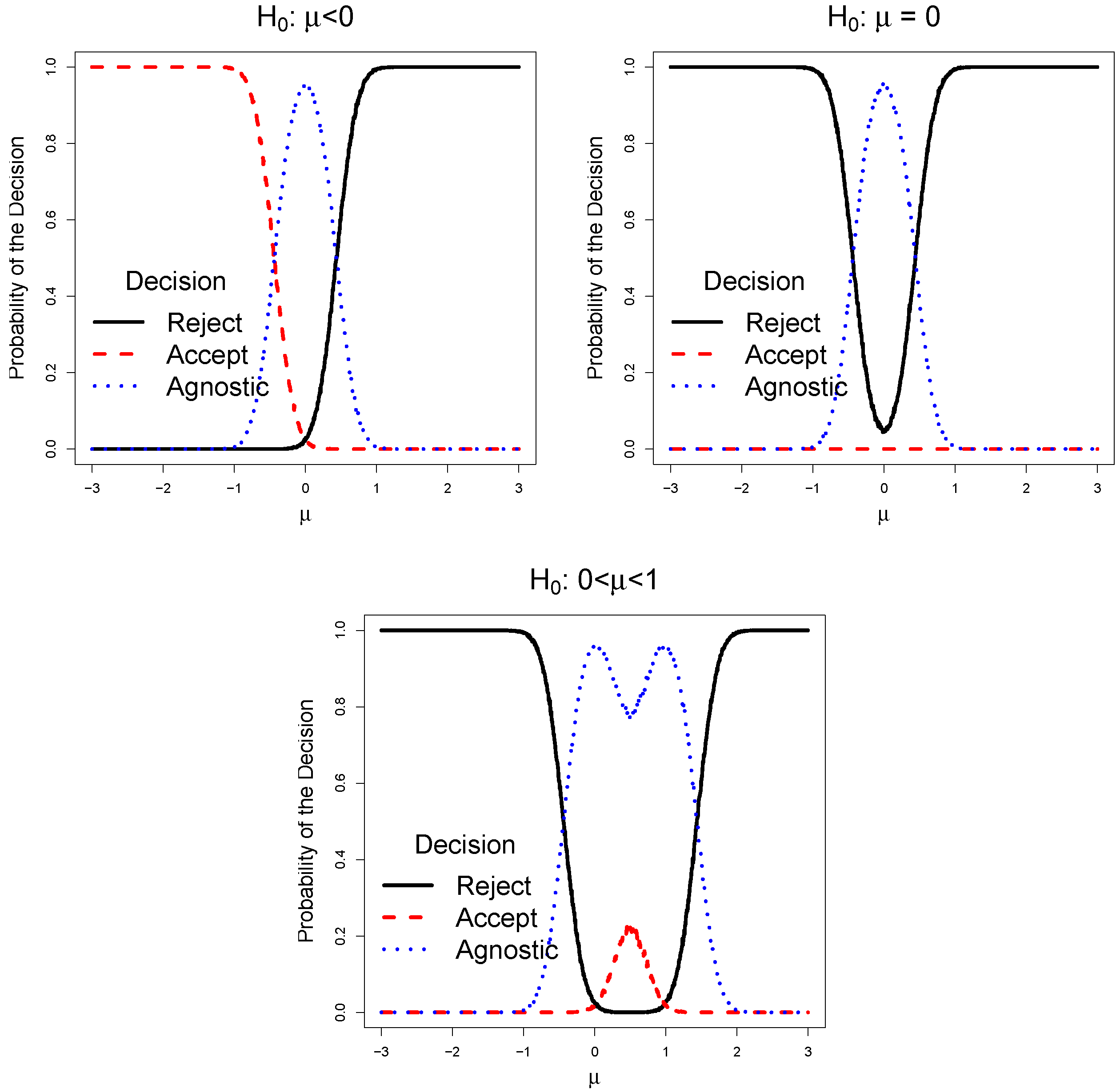
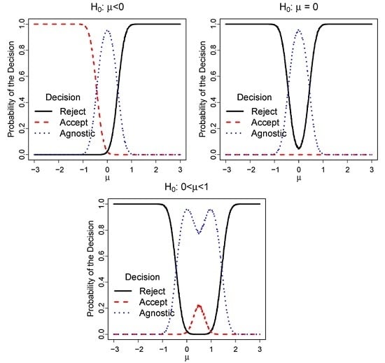
Consider X 1 , , X 20 | μ i . i . d . N o r m a l ( μ , 1 ) . In Figure 2, we illustrate how the probability of each decision, P ( L ( A ) ( X ) = d | μ ) for d { 0 , 1 2 , 1 } , varies as a function of μ for three hypotheses: (i) μ < 0 ; (ii) μ = 0 ; and (iii) 0 < μ < 1 . We consider the standard region estimator for μ, R ( X ) = [ X ¯ z 1 α / 2 1 n ; X ¯ + z 1 α / 2 1 n ] with α = 5 % . These curves represent the generalization of the standard power function to agnostic hypothesis tests. Notice that μ = 0 is never accepted, and that, under the null hypothesis, all tests have at most 5% of probability of rejecting H.
The next two examples show other cases of the ATS in Example 5 that use region estimators based on the measures of evidence in Examples 3 and 4.
Example 7 (Region Likelihood Ratio ATS). 
For a fixed value c ( 0 , 1 ) , define the region estimate R c ( x ) = { θ Θ : λ x ( { θ } ) c } , where λ x is the likelihood ratio statistics from Example 3. For every A σ ( Θ ) and x X , the ATS based on this region estimator (Example 5) satisfies L ( A ) ( x ) = 1 A R c ( x ) = , and L ( A ) ( x ) = 0 A c R c ( x ) = . It follows that this ATS can be written as
L ( A ) ( x ) = 0 if λ x ( A c ) < c 1 if λ x ( A ) < c 1 2 otherwise
Example 8 (Region FBST ATS). 
For a fixed value of c ( 0 , 1 ) , let HPD c x be the Highest Posterior Probability Density region with probability 1 c , based on observation x [3,14]. For every A σ ( Θ ) and x X , the ATS based on this region estimator (Example 5) satisfies L ( A ) ( x ) = 1 A HPD c x = , and L ( A ) ( x ) = 0 A c HPD c x = . It follows that this ATS can be written as
L ( A ) ( x ) = 0 if e v x ( A c ) < c 1 if e v x ( A ) < c 1 2 otherwise
In the sequence, we introduce four logical coherence properties for agnostic testing schemes and investigate which tests satisfy them.

3. Coherence Properties

3.1. Monotonicity

Monotonicity restricts the decisions that are available for nested hypotheses. If hypothesis Aimplies hypothesis B (i.e., A B ), then a testing scheme that rejects B should also reject A. Monotonicity has received a lot of attention in the literature (e.g., [5,6,15,16,17,18,19]). It can be extended to ATS’s in the following way.
Definition 2 (Monotonicity). 
L : σ ( Θ ) Φ is monotonic if, for every A , B σ ( Θ ) , A B implies that L ( A ) L ( B ) .
L is monotonic if, for every hypotheses A B ,
  • if L accepts A, then it also accepts B.
  • if L remains agnostic about A, then it either remains agnostic about B or accepts B.
Next, we illustrate some monotonic agnostic testing schemes.
Example 9 (Tests based on posterior probabilities). 
The ATS from Example 2 is monotonic. Indeed, A B implies that P ( A | x ) P ( B | x ) x X , and hence P ( A | x ) > c i implies that P ( B | x ) > c i for i = 1 , 2 .
Example 10 (Likelihood Ratio Tests with fixed threshold). 
The ATS from Example 3 is monotonic. This is because if A , B σ ( Θ ) are such that A B , then sup θ A L x ( θ ) sup θ B L x ( θ ) , x X , which implies that λ x ( A ) λ x ( B ) . It follows that λ x ( A ) > c i implies that λ x ( B ) > c i for i = 1 , 2 .
Example 11 (FBST). 
The ATS from Example 4 is monotonic. In fact, let A , B σ ( Θ ) be such that A B . We have sup B f ( θ | x ) sup A f ( θ | x ) x X . Hence, T x B T x A , and, therefore, e v x ( A ) e v x ( B ) . It follows that e v x ( A ) > c i implies that e v x ( B ) > c i for i = 1 , 2 .
Notice that p-values and Bayes factors are not (coherent) measures of support for hypotheses [19,20], and therefore using them in a similar fashion as in Examples 2–4 would not lead to monotonic agnostic testing schemes. On the other hand, any monotonic statistic s A does, however, provide a monotonic ATS, because, if A B , s A ( x ) > c i implies that s B ( x ) > c i for i = 1 , 2 . Another example of such statistic is the s-value defined by Patriota [6]. As a matter of fact, every ATS is, in a sense, associated to monotonic statistics as shown in the next theorem.
Theorem 1. 
Let L be an agnostic testing scheme. L is monotonic if, and only if, there exist a sequence of test statistics ( s A ) A σ ( Θ ) , s A : X I R , with s A s B whenever A B , A , B σ ( Θ ) , and cutoffs c 1 , c 2 I , c 1 c 2 , such that for every A σ ( Θ ) and x X ,
L ( A ) ( x ) = 0 i f s A ( x ) > c 1 1 2 i f c 1 s A ( x ) > c 2 1 i f c 2 s A ( x )
Example 12 (Region Estimator). 
The ATS from Example 5 is monotonic, because if A B , A , B σ ( Θ ) , then
L ( A ) ( x ) = I ( R ( x ) A c ) + I ( R ( x ) A ) 2 I ( R ( x ) B c ) + I ( R ( x ) B ) 2 = L ( B ) ( x ) ,
as I ( R ( x ) B c ) I ( R ( x ) A c ) and I ( R ( x ) B ) I ( R ( x ) A ) . Because this ATS is monotonic, it also controls Family Wise Error Rate [21].

3.2. Union Consonance

Finner and Strassburger [4] and Izbicki and Esteves [3] investigated the following logical property, named union consonance: if a (non-agnostic) testing scheme rejects each of the hypotheses A and B, it should also reject their union A B . In other words, a TS cannot accept the union while rejecting its components. In this section, we adapt the concept of union consonance to the framework of agnostic testing schemes by considering two extensions for such desideratum: the weak and the strong union consonance.
Definition 3 (Weak Union Consonance). 
An ATS L : σ ( Θ ) Φ is weakly consonant with the union if, for every A , B σ ( Θ ) , and for every x X ,
L ( A ) ( x ) = 1   and   L ( B ) ( x ) = 1   implies   L ( A B ) ( x ) 0
This is exactly the definition of union consonance for non-agnostic testing schemes. Notice that, according to such definition, it is possible to remain agnostic about A B while rejecting A and B.
Remark 1. 
Izbicki and Esteves [3] show that if a non agnostic testing scheme L satisfies union consonance, then for every finite set of indices I and for every { A i } i I σ ( Θ ) , min { L ( A i ) } i I = 1 implies that L ( i I A i ) 0 . This is not the case for weak union consonant agnostic testing schemes; we leave further details to Section 4.3.
The second definition of union consonance is more stringent than the first one:
Definition 4 (Strong Union Consonance). 
An L : σ ( Θ ) Φ is strongly consonant with the union if, for every arbitrary set of indices I and for every { A i } i I σ ( Θ ) such that i I A i σ ( Θ ) , and for every x X ,
min { L ( A i ) ( x ) } i I = 1   implies   L ( i I A i ) ( x ) = 1
Definition 3 is less stringent than Definition 4 in two senses: (i) the latter imposes the (strict) rejection of a union of hypotheses whenever each of them is rejected while the former imposes just non-acceptance (rejection or abstention) of the union is such circumstances; and (ii) in Definition 4 consonance is required to hold for every set (possibly infinite) of hypotheses as opposed to Definition 3 which applies only to pairs of hypotheses. Notice that if an ATS is strongly consonant with union, it is also weakly consonant with union, and that both definitions are indeed extensions of the concept presented by Izbicki and Esteves [3].
The following examples show ATSs that are consonant with union.
Example 13 (Tests based on posterior probabilities). 
Consider again Example 2 with the restriction c 1 2 c 2 . If A and B are rejected after observing x X , then
P ( A B | x ) P ( A | x ) + P ( B | x ) 2 c 2 c 1 ,
and therefore A B cannot be accepted. Thus, with this restrictions, that ATS is weakly consonant with union. The restriction c 1 2 c 2 is not only sufficient to ensure weak union consonance, but it is actually necessary to ensure it holds for every prior distribution (see Theorem 2). Notice, however, that this ATS is not strongly consonant with union in general.
Example 14 (Likelihood Ratio Tests with fixed threshold). 
The ATS of Example 3 is strongly consonant with union. Indeed, let I be an arbitrary set of indices and { A i } i I σ ( Θ ) be such that i I A i σ ( Θ ) . For every x X , λ x ( i I A i ) = sup i I { λ x ( A i ) } [3]. It follows that if λ x ( A i ) c 2 for every i I , then λ x ( i I A i ) c 2 . Thus, if L rejects all hypotheses A i after x is observed, it also rejects i I A i . In addition, L is also weakly consonant with union.
Example 15 (FBST). 
The ATS from Example 4 is also strongly consonant with union. Indeed, let I be an arbitrary set of indices and { A i } i I σ ( Θ ) be such that i I A i σ ( Θ ) . For every x X , e v x ( i I A i ) = sup i I { e v x ( A i ) } [22]. Strong union consonance holds due to the same argument from Example 14. It follows that L is also weakly consonant with union.
Example 16 (Region Estimator). 
The TS from Example 5 satisfies strong union consonance. Indeed, let I be an arbitrary set of indices and { A i } i I σ ( Θ ) be such that i I A i σ ( Θ ) . If L ( A i ) ( x ) = 1 , then R ( x ) A i c . Hence, if L ( A i ) ( x ) = 1 for every i I , R ( x ) i I A i c = ( i I A i ) c , and, therefore, i I A i is rejected. It follows that L is also weakly consonant with union.

3.3. Intersection Consonance

The third property we investigate, named intersection consonance [3], states that if a (non agnostic) testing scheme cannot accept hypotheses A and B while rejecting its intersection. We consider two extensions of such definition to agnostic testing schemes.
Definition 5 (Weak Intersection Consonance). 
An ATS L : σ ( Θ ) Φ is consonant with the intersection if, for every A , B σ ( Θ ) and x X ,
L ( A ) ( x ) = 0   and   L ( B ) ( x ) = 0   implies   L ( A B ) ( x ) 1 .
This is exactly the definition of intersection consonance for non-agnostic testing schemes. Notice that it is possible to accept A and B while being agnostic about A B .
The second definition of intersection consonance is more stringent:
Definition 6 (Strong Intersection Consonance). 
An ATS L : σ ( Θ ) Φ is strongly consonant with the intersection if, for every arbitrary set of indices I and for every { A i } i I σ ( Θ ) such that i I A i σ ( Θ ) , and for every x X ,
max { L ( A i ) ( x ) } i I = 0   implies   L ( i I A i ) ( x ) = 0 .
As in the case of union consonance, Definition 5 is less stringent than Definition 6 in two senses: (i) the latter imposes the (strict) acceptance of an intersection of hypotheses whenever each of them is accepted while the former imposes just non-rejection (acceptance or abstention) of the intersection is such circumstances; and (ii) in Definition 6 consonance is required to hold for every set (possibly infinite) of hypotheses as opposed to Definition 5 which applies only to pairs of hypotheses. Notice that if an ATS is strongly consonant with intersection, it is also weakly consonant with intersection, and that both definitions are indeed extensions of the concept presented by Izbicki and Esteves [3].
Example 17 (Tests based on posterior probabilities). 
Consider Example 2 with the restriction c 2 2 c 1 1 . If A and B are accepted when x X is sampled, then P ( A | x ) > c 1 and P ( B | x ) > c 1 . By Fréchet inequality, it follows that
P ( A B | x ) P ( A | x ) + P ( B | x ) 1 > 2 c 1 1 c 2
and, therefore, A B cannot be rejected. It follows that weak intersection consonance holds. The restriction c 2 2 c 1 1 is not only sufficient to ensure weak intersection consonance, but it is actually necessary to ensure this property holds for every prior distribution; see Theorem 2. Notice, however, that this ATS is not strongly consonant with intersection in general (Take, for example, Θ = [ 0 , 1 ] , P = λ (the Lebesgue measure), A = [ 0 , 2 / 3 ] , B = [ 1 / 3 , 1 ] , and c 1 = 3 / 5 ).
The ATS based on the likelihood ratio statistic from Example 3 does not satisfy intersection consonance, because there are examples in which λ x ( A B ) = 0 , while λ x ( A ) > 0 and λ x ( B ) > 0 (Consider, for example, that every θ Θ has the same likelihood and A B = ). Similarly, the ATS based on FBST from Example 4 is not consonant with intersection, because there are examples such that e v x ( A B ) = 0 , while e v x ( A ) > 0 and e v x ( B ) > 0 . ATSs based on region estimators are consonant with intersection.
Example 18 (Region Estimator). 
The TS from Example 5 satisfies both strong and weak intersection consonance. Indeed, let I be an arbitrary set of indices and { A i } i I σ ( Θ ) be such that i I A i σ ( Θ ) . If L ( A i ) ( x ) = 0 for every i I , then R ( x ) A i for every i I . It follows that R ( x ) i I A i , and hence i I A i is accepted.
It follows that the ATSs from Examples 7 and 8 are are also consonant with intersection. Hence, it is possible to use e-values and likelihood ratio statistics to define ATS that are consonant with intersection.
Example 19 (ANOVA). 
In [3], the authors present an example which we now revisit. Suppose that X 1 , , X 20 are i.i.d. N ( μ 1 , σ 2 ) ; X 21 , , X 40 are i.i.d. N ( μ 2 , σ 2 ) and X 41 , , X 60 are i.i.d. N ( μ 3 , σ 2 ) . Consider the following hypotheses:
H 0 ( 1 , 2 , 3 ) : μ 1 = μ 2 = μ 3 H 0 ( 1 , 2 ) : μ 1 = μ 2 H 0 ( 1 , 3 ) : μ 1 = μ 3
and suppose that we observe the following means and standard-deviations on the data: X ¯ 1 = 0 . 15 ; S 1 = 1 . 09 ; X ¯ 2 = 0 . 13 ; S 2 = 0 . 5 X ¯ 3 = 0 . 38 ; S 3 = 0 . 79 . Using the likelihood ratio statistics, we have the following p-values for these hypotheses:
p H 0 ( 1 , 2 , 3 ) = 0 . 0498 p H 0 ( 1 , 2 ) = 0 . 2564 p H 0 ( 1 , 3 ) = 0 . 0920
Therefore, the testing scheme given by the likelihood ratio tests with common level of significance α = 5 % rejects H 0 ( 1 , 2 , 3 ) but does not reject either H 0 ( 1 , 2 ) or H 0 ( 1 , 3 ) . It follows intersection consonance does not hold. Now, consider the region estimator ATS based on the region estimate given by [23] for this setting,
R ( x ) = ( μ 1 , μ 2 , μ 3 ) R 3 : μ 1 μ 2 1 . 65 , 2 . 21 , μ 2 μ 3 1 . 68 , 2 . 18 , μ 1 μ 3 1 . 40 , 2 . 46
All hypotheses H 0 ( 1 , 2 , 3 ) , H 0 ( 1 , 2 ) , and H 0 ( 1 , 3 ) intercept both R ( x ) and its complement, so that one remains agnostic about all of them. As expected, intersection consonance holds using this ATS.

3.4. Invertibility

Invertibility formalizes the notion of simultaneous tests free from the labels “null” and “alternative” for the hypotheses of interest and has been suggested by several authors, specially under a Bayesian perspective [3,24,25].
Definition 7 (Invertibility). 
An ATS L : σ ( Θ ) Φ is invertible if, for every A σ ( Θ ) ,
L ( A c ) = 1 L ( A )
Example 20 (Tests based on posterior probabilities). 
The ATS from Example 2 is invertible for every prior distribution if and only if c 2 = 1 c 1 .
Example 21 (Region Estimator). 
The ATS from Example 5 is invertible. Indeed,
L ( A ) ( x ) = I ( R ( x ) A c ) + I ( R ( x ) A ) ) 2 = ( 1 I ( R ( x ) A c ) ) + ( 1 I ( R ( x ) A ) ) 2 = 1 L ( A c ) ( x )
It follows that the ATS from Examples 7 and 8 are also invertible.

4. Satisfying All Properties

Is it possible to construct non-trivial agnostic testing schemes that satisfy all consistency properties simultaneously? Contrary to the case of non agnostic testing schemes [3], the answer is yes. We next examine this question considering three desiderata: the weak desiderata (Section 4.1), the strong desiderata (Section 4.2), and the n-weak desiderata (Section 4.3).

4.1. Weak Desiderata

Definition 8 (Weakly Consistent ATS). 
An ATS, L , is said to be weakly consistent if L is monotonic (Definition 2), invertible (Definition 7), weakly consonant with the union (Definition 3), and weakly consonant with the intersection (Definition 5).
Example 22 (Region Estimator). 
The ATS from Example 5 was already shown to satisfy all consistency properties from Definition 8 (Examples 12, 16, 18 and 21). Thus, it is a weakly consistent ATS.
It follows that the ATSs Examples 7 and 8, based on measures of support (likelihood ratio statistics and e-values), are weakly consistent ATSs.
Example 23 (Tests based on posterior probabilities). 
Consider Example 2. We have seen that the following restrictions are sufficient to guarantee union weak consonance (Example 13), weak intersection consonance (Example 17) and invertibility (Example 20), respectively: c 1 2 c 2 , 2 c 1 1 c 2 and c 2 = 1 c 1 . It follows from these relations and the fact that this ATS is monotonic (Example 9) that if c 1 > 2 / 3 and c 2 = 1 c 1 , then it is weakly consistent, whatever the prior distribution for θ is.
The next theorem shows necessary and sufficient conditions for agnostic tests based on posterior distribution (with possibly different thresholds c 1 and c 2 for each hypothesis of interest) to satisfy each of the coherence properties.
Theorem 2. 
Let Θ = R d and σ ( Θ ) = B ( Θ ) , the Borelians of R d . Let P be a prior probability measure in σ ( Θ ) . For each A σ ( Θ ) , let L ( A ) : X D be defined by
L ( A ) ( x ) = 0 i f P ( A | x ) > c 1 A 1 2 i f c 1 A P ( A | x ) > c 2 A 1 i f c 2 A P ( A | x )
where P ( . | x ) is the posterior distribution of θ, given x, and 0 c 2 A c 1 A 1 . This is a generalization of the ATS of Example 2. Assume that the likelihood function is positive for every x X and θ Θ . Such ATS satisfies:
1. 
Monotonicity for every prior distribution if, and only if, for every A , B σ ( Θ ) with A B , c 2 A c 2 B and c 1 A c 1 B
2. 
Weak union consonance for every prior distribution if, and only if, for every A , B σ ( Θ ) such that A B , c 2 A + c 2 B c 1 A B
3. 
Weak intersection consonance for every prior distribution if, and only if, for every A , B σ ( Θ ) such that A B , c 1 A + c 1 B 1 c 2 A B
4. 
Invertibility for every prior distribution if, and only if, for every A σ ( Θ ) , c 1 A = 1 c 2 A c
It follows from Theorem 2 that if the cutoffs used in each of the tests ( c 1 and c 2 ) are required to be the same for all hypothesis of interest, then the conditions in Example 23 are not only sufficient, but they are also necessary to ensure that all (weak) consistency properties hold for every prior distribution for θ.

4.2. Strong Desiderata

Definition 9 (Fully Consistent ATS). 
An ATS, L , is said to be fully consistent if L is monotonic (Definition 2), invertible (Definition 7), strongly consonant with the union (Definition 4), and strongly consonant with the intersection (Definition 6).
The following theorem shows that, under mild assumptions, the only ATSs that are fully consistent are those based on region estimators.
Theorem 3. 
Assume that for every θ Θ , { θ } σ ( Θ ) . An ATS is fully consistent if, and only if, it is a region estimator-based ATS (Example 5).
Hence, the only way to create a fully consistent ATS is by designing an appropriate region estimator and using Example 5. In particular, ATSs based on posterior probabilities (Example 2) are typically not fully consistent. It should be emphasized that when the region estimator that characterizes a fully consistent ATS L maps X to singletons of Θ, no sample point will lead to abstention, as either R ( x ) A or R ( x ) A c , for every A σ ( Θ ) . In such situations, region estimators reduce to point estimator which charaterize full consistent non-agnostic TSs [3].
In the next section, we consider a desiderata for simultaneous tests which is not as strong as that of Definition 9, but which is more stringent that that of Definition 8.

4.3. n-Weak Desiderata

In Section 3.2 and Section 3.3, weak consonance was defined for two hypotheses only. It is however possible to define it for n < hypotheses:
Definition 10 (Weak n-union Consonance) 
An A-TS L : σ ( Θ ) Φ satisfies weak n-union consonant if, for every finite set of indices I, with | I | n , for every { A i } i I σ ( Θ ) , and for every x X
min { L ( A i ) ( x ) } i I = 1   implies   L ( i I A i ) ( x ) 0 .
Definition 11 (Weak n-intersection Consonance) 
An ATS L : σ ( Θ ) Φ is weak n-intersection consonant if, for every finite set of indices I, with | I | n , for every { A i } i I σ ( Θ ) , and for every x X
max { L ( A i ) ( x ) } i I = 0   implies   L ( i I A i ) ( x ) 1 .
Although in the context of non agnostic testing schemes (union or intersection) consonance holds for n = 2 if, and only if, it holds for every n N [3], this is not the case in the agnostic setting. We hence define
Definition 12 (n-Weakly Consistent ATS) 
An ATS, L , is said to be n-weakly consistent if L is monotonic (Definition 2), invertible (Definition 7), n-weakly consonant with the union (Definition 10), and n-weakly consonant with the intersection (Definition 11).
Example 24 (Region Estimator). 
The ATS from Example 5 satisfies weak n-union and weak n-intersection consonance. The argument is the same as that presented in Examples 16 and 18. It follows that this is a n-weakly consistent ATS.
Example 25 (Tests based on posterior probabilities). 
Consider Example 2. In order to guarantee weak n-union consonance for every prior, it is necessary and sufficient to have c 1 n c 2 . Moreover, to guarantee weak n-intersection consonance for every prior, it is necessary and sufficient to have c 2 n c 1 ( n 1 ) . It follows from these conditions and Example 20 that the following restrictions are necessary and sufficient to guarantee monotonicity, n-union consonance, n-intersection consonance and invertibility: c 1 > n / ( n + 1 ) and c 2 = 1 c 1 . Hence, these conditions are sufficient to guarantee this ATS is n-weakly consistent. Now, because these conditions are also necessary, it follows that this ATS is n-weakly consistent for every n > 1 if, and only if, it remains agnostic about every hypothesis which has probability in ( 0 , 1 ) .

5. Decision-Theoretic Perspective

In this section, we investigate agnostic testing schemes from a Bayesian decision-theoretic perspective. First, we define an ATS generated by a family of loss functions. Note that, in the context of agnostic tests, a loss function is a function L : D × Θ R that assigns to each θ Θ the loss L ( d , θ ) for making the decision d { 0 , 1 2 , 1 } .
Definition 13 (ATS generated by a family of loss functions). 
Let ( X × Θ , σ ( X × Θ ) , P ) be a Bayesian statistical model. Let ( L A ) A σ ( Θ ) be a family of loss functions, where L A : D × Θ R is the loss function to be used to test A σ ( Θ ) . An ATS generated by the family of loss functions ( L A ) A σ ( Θ ) is any ATS L defined over the elements of σ ( Θ ) such that, A σ ( Θ ) , L ( A ) is a Bayes test for hypothesis A against P .
Example 26 (Bayesian ATS generated by a family of error-wise constant loss functions). 
For A σ ( Θ ) , consider the loss function L A of the form of Table 1, where all entries are assumed to be non negative. This is a generalization of standard 0 1 c loss functions to agnostic tests in the sense that it penalizes not only false acceptance and false rejection with constant losses b A and d A , respectively, but also an eventual abstention from deciding between accepting and rejecting A with the values a A and c A . If b A d A > a A b A + c A d A , then the Bayes test against L A consists in rejecting A if P ( A | x ) < c A d A + c A a A , accept A if P ( A | x ) > b A c A a A + b A c A , and remain agnostic otherwise. It follows that the following ATS is generated by the family of loss functions ( L A ) A σ ( Θ ) :
L ( A ) ( x ) = 0 if P ( A | x ) > b A c A a A + b A c A 1 2 if b A c A a A + b A c A P ( A | x ) > c A d A + c A a A 1 if c A d A + c A a A P ( A | x )
Notice that if, for every A , B σ ( Θ ) , a A = a B , b A = b B , c A = c B , and d A = d B , this ATS matches that from Example 2 for a particular value of c 1 and c 2 .
We restrict out attention to ATSs generated by proper losses, a concept we adapt from [3] to agnostic tests:
Definition 14 (Proper losses). 
A family of loss functions ( L A ) A σ ( Θ ) has proper losses if
L A ( 0 , θ ) < L A ( 1 2 , θ ) < L A ( 1 , θ ) , if θ A L A ( 0 , θ ) > L A ( 1 2 , θ ) > L A ( 1 , θ ) , if θ A L A ( 1 2 , θ ) < L A ( 0 , θ ) + L A ( 1 , θ ) 2 , for all θ
Definition 14 states that (i) by taking a correct decision we lose less than by taking a wrong decision; (ii) by remaining agnostic we do not lose as much as when taking a wrong decision, but we lose more than by taking a correct decision; and (iii) it is better to remain agnostic about A than to flip a coin to decide if we reject or accept this hypothesis.
Example 27 (Bayesian ATS generated by a family of error-wise constant loss functions). 
In order to ensure that the loss in Example 26 is proper, the following restrictions must be satisfied: 0 < a A < d A / 2   and   0 < c A < b A / 2 . In particular, these conditions imply those stated in Example 26.

5.1. Monotonicity

We now turn our attention towards characterizing Bayesian monotonic ATS using a decision-theoretic framework. In order to do this, we first adapt the concept of relative losses [3] to the context of agnostic testing schemes.
Definition 15 (Relative Loss). 
Let L A be a loss function for testing hypothesis A. The relative losses r A ( 1 , 1 2 ) : Θ R and r A ( 1 2 , 0 ) : Θ R are defined by
r A ( 1 , 1 2 ) ( θ ) = L A ( 1 , θ ) L A ( 1 2 , θ ) r A ( 1 2 , 0 ) ( θ ) = L A ( 1 2 , θ ) L A ( 0 , θ )
The relative losses thus measure the difference between the losses of rejecting a given hypothesis and remaining agnostic about it, as well as the difference between the losses of remaining agnostic and accepting it. In order to guarantee that a Bayesian ATS is monotonic, certain constraints on the relative losses must be imposed. The next definition presents one of such assumptions, which we interpret in the sequence.
Definition 15 (Relative Loss). 
Let D > 2 = { ( 1 , 1 2 ) , ( 1 2 , 0 ) } . ( L A ) A σ ( Θ ) has monotonic relative losses if the family ( L A ) A σ ( Θ ) is proper and, for all A , B σ ( Θ ) such that A B and for all ( i , j ) D > 2 ,
r B ( i , j ) ( θ ) r A ( i , j ) ( θ ) θ Θ
Let A , B σ ( Θ ) with A B . If θ A , both A and B are true, so ( L A ) A σ ( Θ ) having monotonic relative losses reflects the situation in which the rougher error of rejecting B compared to rejecting A (with respect to remaining agnostic about these hypotheses) should be assigned a larger relative loss. Similarly, the rougher error of remaining agnostic about B should be assigned a larger relative loss than remaining agnostic about A (with respect to correctly accepting these hypotheses). If θ B but θ A , these conditions are a consequence of the assumption that the family ( L A ) A σ ( Θ ) is proper. The case θ B can be interpreted in a similar fashion as the case θ A .
The following example presents necessary and sufficient conditions to ensure that the loss functions from Example 26 yield monotonic relative losses.
Example 28. 
Consider the losses presented in Example 26. Assuming the losses are proper (see Example 27), the conditions required to ensure ( L A ) A σ ( Θ ) has monotonic relative losses are
a A a B , c B c A , c B b B c A b A  and  d B a B d A a A
Notice that these restrictions imply that b A b B .
As a particular example, let k > 2 and λ be a finite measure in σ ( Θ ) with λ ( Θ ) > 0 . The following assignments yield a proper and monotonic loss: for every A σ ( Θ ) , b A = λ ( A c ) , a A = λ ( A ) / k , c A = λ ( A c ) / k , and d A = λ ( A ) . Another particular case is when a A = a B , b A = b B , c A = c B , and d A = d B for every A , B σ ( Θ ) .
Another concept that helps us characterizing the Bayesian monotonic agnostic testing schemes is that of balanced relative losses, which we adapt from [7].
Definition 17 (Balanced Relative Loss). 
( L A ) A σ ( Θ ) has balanced relative losses if, for all A , B σ ( Θ ) such that A B , for all θ 1 A and θ 2 B c , and for all ( i , j ) D > 2 ,
r A ( i , j ) ( θ 1 ) r A ( i , j ) ( θ 2 ) r B ( i , j ) ( θ 1 ) r B ( i , j ) ( θ 2 )
Lemma 1. 
If ( L A ) A σ ( Θ ) has monotonic relative losses, then ( L A ) A σ ( Θ ) has balanced relative losses.
The following result shows that balanced relative losses characterize Bayesian monotonic ATS.
Theorem 4. 
Let ( L A ) A σ ( Θ ) be a family of proper loss functions. Assume that for every θ Θ and x X , L x ( θ ) > 0 . For every prior π for θ, let L π denote a Bayesian ATS generated by ( L A ) A σ ( Θ ) . There exists a monotonic L π for every prior π if, and only if, ( L A ) A σ ( Θ ) has balanced relative losses.
Example 29. 
In Example 28, we obtained conditions on the loss functions ( L A ) A σ ( Θ ) from Example 26 in order to guarantee that family to have monotonic relative losses. From Lemma 1 and Theorem 4, it follows that such family of loss functions yield monotonic Bayesian ATSs whatever the prior for θ is. In other words, there are family of loss functions that induce monotonic tests based on posterior probabilities.

5.2. Union Consonance

We now turn our attention towards characterizing union consonant Bayesian ATS using a decision theoretic framework.
Definition 18. 
( L A ) A σ ( Θ ) is compatible with weak union consonance if there exists no A , B σ ( Θ ) , θ 1 , θ 2 , θ 3 Θ and p 1 , p 2 , p 3 0 such that p 1 + p 2 + p 3 = 1 and
p 1 · r A ( 1 , 1 2 ) ( θ 1 ) + p 2 · r A ( 1 , 1 2 ) ( θ 2 ) + p 3 · r A ( 1 , 1 2 ) ( θ 3 ) < 0 p 1 · r B ( 1 , 1 2 ) ( θ 1 ) + p 2 · r B ( 1 , 1 2 ) ( θ 2 ) + p 3 · r B ( 1 , 1 2 ) ( θ 3 ) < 0 p 1 · r A B ( 1 2 , 0 ) ( θ 1 ) + p 2 · r A B ( 1 2 , 0 ) ( θ 2 ) + p 3 · r A B ( 1 2 , 0 ) ( θ 3 ) > 0
Definition 18 states that the family of loss functions ( L A ) A σ ( Θ ) being compatible with weak union consonance cannot induce any Bayesian ATS on the basis of which one may prefer rejecting both hypotheses A and B over remaining agnostic about them while accepting A B rather than abstaining.
As we will see in the next theorem, proper loss functions compatible with weak union consonance characterize Bayesian ATSs that are weakly consonant with the union.
Theorem 5. 
Let ( L A ) A σ ( Θ ) be a family of proper loss functions. Assume that for every θ Θ and x X , L x ( θ ) > 0 . For every prior π for θ, let L π denote a Bayesian ATS generated by ( L A ) A σ ( Θ ) . There exists an ATS L π that is weakly consonant with the union for every priori π if, and only if, ( L A ) A σ ( Θ ) is compatible with weak union consonance.
Example 30. 
We saw that the ATS from Example 2 is a Bayes test against a particular proper loss (Examples 26 and 27) and that it is weakly consonant with the union (Example 13). It follows from Theorem 5 that the family of loss functions that lead to this ATS are compatible with weak union consonance.
Definition 19 (Union consonance-balanced relative losses [7]). 
( L A ) A σ ( Θ ) has union consonance-balanced relative losses if, for every A , B σ ( Θ ) , θ 1 A B and θ 2 ( A B ) c ,
r A ( 1 , 1 2 ) ( θ 1 ) r A ( 1 , 1 2 ) ( θ 2 ) r A B ( 1 2 , 0 ) ( θ 1 ) r A B ( 1 2 , 0 ) ( θ 2 ) , or r B ( 1 , 1 2 ) ( θ 1 ) r B ( 1 , 1 2 ) ( θ 2 ) r A B ( 1 2 , 0 ) ( θ 1 ) r A B ( 1 2 , 0 ) ( θ 2 )
Corollary 1. 
Let ( L A ) A σ ( Θ ) be a family of proper loss functions. Assume that for every θ Θ and x X , L x ( θ ) > 0 . If ( L A ) A σ ( Θ ) does not have union consonance-balanced relative losses, then there exists a prior π such that every Bayesian ATS, L π , is not weakly consonant with the union.

5.3. Intersection Consonance

Next, we characterize intersection consonant Bayesian ATS under a Bayesian perspective.
Definition 20. 
( L A ) A σ ( Θ ) is compatible with weak intersection consonance if there exists no A , B σ ( Θ ) , θ 1 , θ 2 , θ 3 Θ and p 1 , p 2 , p 3 0 such that p 1 + p 2 + p 3 = 1 and
p 1 · r A ( 1 2 , 0 ) ( θ 1 ) + p 2 · r A ( 1 2 , 0 ) ( θ 2 ) + p 3 · r A ( 1 2 , 0 ) ( θ 3 ) > 0 p 1 · r B ( 1 2 , 0 ) ( θ 1 ) + p 2 · r B ( 1 2 , 0 ) ( θ 2 ) + p 3 · r B ( 1 2 , 0 ) ( θ 3 ) > 0 p 1 · r A B ( 1 , 1 2 ) ( θ 1 ) + p 2 · r A B ( 1 , 1 2 ) ( θ 2 ) + p 3 · r A B ( 1 , 1 2 ) ( θ 3 ) < 0
Definition 20 states that the family of loss functions ( L A ) A σ ( Θ ) being compatible with weak intersection consonance cannot induce any Bayesian ATS on the basis of which one may prefer accepting both hypotheses A and B to remaining agnostic about them while rejecting A B rather than abstaining.
As we will see in the next theorem, proper loss functions compatible with weak intersection consonance characterize Bayesian ATSs that are weakly consonant with the intersection .
Theorem 6. 
Let ( L A ) A σ ( Θ ) be a family of proper loss functions. Assume that for every θ Θ and x X , L x ( θ ) > 0 . For every prior π for θ, let L π denote a Bayesian ATS generated by ( L A ) A σ ( Θ ) . There exists an ATS L π that is weakly consonant with the intersection for every prior π if, and only if, ( L A ) A σ ( Θ ) is compatible with weak intersection consonance.
Example 31. 
We saw that the ATS from Example 2 is a Bayes test against a particular proper loss (Examples 26 and 27) and that it is weakly consonant with the intersection (Example 17). It follows from Theorem 6 that the family of loss functions that lead to this ATS are compatible with weak intersection consonance.
Definition 21 (Intersection consonance-balanced relative losses [7]). 
( L A ) A σ ( Θ ) has intersection consonance-balanced relative losses if, for every A , B σ ( Θ ) , θ 1 A B and θ 2 ( A B ) c ,
r A B ( 1 , 1 2 ) ( θ 1 ) r A B ( 1 , 1 2 ) ( θ 2 ) r A ( 1 2 , 0 ) ( θ 1 ) r A ( 1 2 , 0 ) ( θ 2 ) , or r A B ( 1 , 1 2 ) ( θ 1 ) r A B ( 1 , 1 2 ) ( θ 2 ) r B ( 1 2 , 0 ) ( θ 1 ) r B ( 1 2 , 0 ) ( θ 2 )
Corollary 2. 
Let ( L A ) A σ ( Θ ) be a family of proper loss functions. Assume that for every θ Θ and x X , L x ( θ ) > 0 . If ( L A ) A σ ( Θ ) does not have intersection consonance-balanced relative losses, then there exists a prior π such that every Bayesian ATS, L π , is not weakly consonant with the intersection.
We end this section by noting that although we focused our results on weak consonance, they can be extended to strong consonance using the same techniques presented in the Appendix.

5.4. Invertibility

Finally, we examine invertible Bayesian ATSs from a decision-theoretic standpoint.
Definition 22 (Invertible Relative Losses). 
( L A ) A σ ( Θ ) has invertible relative losses if, for every A σ ( Θ ) , for all θ 1 A , θ 2 A c and ( i , j ) D > 2 ,
r A ( i , j ) ( θ 1 ) r A ( i , j ) ( θ 2 ) = r A c ( i , j ) ( θ 1 ) r A c ( i , j ) ( θ 2 )
We end this section by showing that invertible Bayesian ATSs are determined by family of loss functions that fulfill the conditions of Definition 22.
Theorem 7. 
Let ( L A ) A σ ( Θ ) be a family of proper loss functions. Assume that for every θ Θ and x X , L x ( θ ) > 0 . For every prior π for θ, let L π denote a Bayesian ATS generated by ( L A ) A σ ( Θ ) . There exists an ATS L π that is invertible for every prior π if, and only if, ( L A ) A σ ( Θ ) has invertible relative losses.
Example 32. 
For every A σ ( Θ ) , let ( L A ) A σ ( Θ ) be such that L A ( 1 , θ ) = L A c ( 0 , θ ) and L A ( 1 2 , θ ) = L A c ( 1 2 , θ ) . It is easily seen that the conditions from Definition 22 hold. Theorem 7 then implies that any Bayesian ATS generated by ( L A ) A σ ( Θ ) is invertible.

6. Final Remarks

Agnostic tests allow one to explicitly capture the difference between “not rejecting” and “accepting” a null hypothesis. When the agnostic decision is chosen, the null hypothesis is neither rejected or accepted. This possibility aligns with the idea that although precise null hypotheses can be tested, they shouldn’t be accepted. This idea is followed by the region based agnostic tests derived in this paper, which can either remain agnostic or reject precise null hypotheses.
This distinction provides a solution to the problem raised by Izbicki and Esteves [3], in which all (non-agnostic) logically coherent tests were shown to be based on point estimators which lack statistical optimality. We show that agnostic tests based on region estimators satisfy logical consistency and also allow statistical optimality. For example, agnostic tests based on frequentist confidence intervals control family wise error. Similarly, agnostic tests based on posterior density regions are shown to be an extension of the Full Bayesian Significance Test [11].
Future research includes investigating the consequences and generalizations of the logical requirements in this paper. For example, one could study what kinds of trivariate logic derive from the different definition of logical consistency studied in this paper. One could also generalize these logical requirements to generalized agnostic tests, in which one can decide among different degrees of agnosticism. The scale of such degrees can be either discrete or continuous. One could also investigate region estimator-based ATSs with respect to other optimality criteria such as statistical power.
The results of this paper can also be tied to the philosophical literature that studies the consequences and importance of precise hypothesis. Agnostic tests can be used to revisit the role of testing precise hypotheses in science. Agnostic tests also provide a framework to interpret the scientific meaning of measures of possibility or significance of precise hypotheses.
multiple

Acknowledgments

Julio M. Stern is grateful for the support of IME-USP, the Institute of Mathematics and Statistics of the University of São Paulo; FAPESP—the State of São Paulo Research Foundation (grants CEPID 2013/07375-0 and 2014/50279-4); and CNPq—the Brazilian National Counsel of Technological and Scientific Development (grant PQ 301206/2011-2). Rafael Izbicki is grateful for the support of FAPESP (grant 2014/25302-2).

Author Contributions

The manuscript has come to fruition by the substantial contributions of all authors. All authors have also been involved in either writing the article or carefully revising it. All authors have read and approved the submitted version of the paper.

Conflicts of Interest

The authors declare no conflict of interest.

Appendix A

Proof of Theorem 1. 
The sufficiency is immediate. Let I = { 0 , 1 2 , 1 } R , c 1 = 1 2 and c 2 = 0 . For A σ ( Θ ) , let s A = 1 L ( A ) , ( s A ) A σ ( Θ ) is such that s A ( x ) s B ( x ) , x X , if A B and it is straightforward to verify Equation (1).
Now, let A , B σ ( Θ ) , with A B . If L is given by Equation (1), it follows that:
  • L A ( x ) = 0 s A ( x ) > c 1 s B ( x ) > c 1 L B ( x ) = 0 .
  • L A ( x ) = 1 2 c 1 s A ( x ) > c 2 s B ( x ) > c 2 L B ( x ) { 0 , 1 2 } .
  • L A ( x ) = 1 L B ( x ) L A ( x ) = 1 .
From ( 1 ) , ( 2 ) , ( 3 ) it follows that L A ( x ) L B ( x ) , thus L is monotonic.  ☐
Proof of Theorem 2. 
We start by proving the sufficiency of these conditions.
  • If for every A , B σ ( Θ ) with A B , c 2 A c 2 B and c 1 A c 1 B , then for every x X , P ( A | x ) > c 2 A P ( B | x ) > c 2 B , and P ( A | x ) > c 1 A P ( B | x ) > c 1 B . It follows that monotonicity holds.
  • If for every A , B σ ( Θ ) such that A B , c 2 A + c 2 B c 1 A B , then for every x X , P ( A | x ) c 2 A and P ( B | x ) c 2 B implies that P ( A B | x ) P ( A | x ) + P ( B | x ) = c 2 A + c 2 B c 1 A B . It follows that union consonance holds.
  • If for every A , B σ ( Θ ) such that A B , c 1 A + c 1 B 1 c 2 A B , then for every x X , P ( A | x ) > c 1 A and P ( B | x ) > c 1 B implies that P ( A B | x ) P ( A | x ) + P ( B | x ) 1 > c 1 A + c 1 B 1 c 2 A B . It follows that intersection consonance holds.
  • If for every A σ ( Θ ) , c 1 A = 1 c 2 A c , then for every x X , P ( A | x ) c 1 A if, and only if, P ( A c | x ) 1 c 1 A = c 2 A c . Similarly, P ( A | x ) c 2 A if, and only if, P ( A c | x ) 1 c 2 A = c 1 A c . It follows that invertibility holds.
We prove the necessary condition only for union consonance; the other statements have a similar proof. Suppose there are A , B σ ( Θ ) , A B , such that c 2 A + c 2 B > c 1 A B . Let θ 1 A B c and θ 2 B A c .
First, assume c 2 A + c 2 B 1 . Let ϵ > 0 be such that ϵ ( c 2 A + c 2 B c 1 A B ) / 2 and ϵ < min { c 2 A , c 2 B } . Assume that the posterior distribution on Θ given x is such that
P ( A | x ) = P ( { θ 1 } | x ) = c 2 A ϵ  and  P ( B | x ) = P ( { θ 2 } | x ) = c 2 B ϵ
(see the Appendix of [3] for a prior distribution that leads to such posterior). It follows that P ( A | x ) = P ( { θ 1 } | x ) c 2 A , P ( B | x ) = P ( { θ 2 } | x ) c 2 B , and
P ( A B | x ) = P ( { θ 1 } | x ) + P ( { θ 2 } | x ) = c 2 A + c 2 B 2 ϵ > c 2 A + c 2 B ( c 2 A + c 2 B c 1 A B ) = c 1 A B
Hence A and B are rejected, but A B is accepted.
Now, assume c 2 A + c 2 B > 1 . Let b 2 A < c 2 A and b 2 B < c 2 B be such that b 2 A + b 2 B = 1 . Assume that the posterior distribution on Θ is such that
P ( A | x ) = P ( { θ 1 } | x ) = b 2 A  and  P ( B | x ) = P ( { θ 2 } | x ) = b 2 B
It follows that P ( A | x ) = P ( { θ 1 } | x ) < b 2 A < c 2 A , P ( B | x ) = P ( { θ 2 } | x ) < b 2 B < c 2 B , and
P ( A B | x ) = P ( { θ 1 } , { θ 2 } | x ) = b 2 A + b 2 B = 1 c 1 A B
Hence A and B are rejected, but A B is not.  ☐
Lemma A1. 
Let L be an invertible ATS. If, for every x, there exists R ( x ) Θ such that A σ ( Θ ) L ( A ) ( x ) = 0 if and only if R ( x ) A , then L is a region estimator-based ATS (Example 5).
Proof of Lemma A1. 
It follows from definition that, for every A σ ( Θ ) such that R ( x ) A , L ( A ) ( x ) = 0 . Furthermore, for every A σ ( Θ ) such that R ( x ) A c , L ( A c ) ( x ) = 0 . Therefore, it follows from invertibility that L ( A ) ( x ) = 1 . Finally, let A σ ( Θ ) be such that A R ( x ) and A C R ( x ) . Since A R ( x ) R ( x ) and A c R ( x ) R ( x ) it follows that L ( A ) ( x ) 1 2 and L ( A c ) ( x ) 1 2 . Conclude from invertibility that L ( A ) ( x ) = 1 2 .  ☐
Proof of Theorem 3. 
It follows from definition that a region estimator ATS is fully consistent. In order to prove the reverse implication, consider the following notation. For every x X and θ Θ , let A θ = Θ { θ } . Let R ( x ) = { A θ : L ( A θ ) ( x ) = 0 } .
Next, we prove that, for every B σ ( Θ ) , L ( B ) ( x ) = 0 if and only if R ( x ) B . Let B σ ( Θ ) be such that R ( x ) B . Therefore, it follows from the definition of R ( x ) that, for every θ B c , L ( A θ ) = 0 . Since B = { A θ : θ B c } , it follows from strong intersection consonance (Definition 6) that L ( B ) ( x ) = 0 . Let B σ ( Θ ) be such that L ( B ) ( x ) = 0 . It follows from the monotonicity of L (Definition 2) that, for every θ B c , L ( A θ ) ( x ) = 0 as B A θ . Therefore,
R ( x ) = { A θ : L ( A θ ) ( x ) = 0 } { A θ : θ B c } = B
Conclude that for every B σ ( Θ ) , L ( B ) ( x ) = 0 if and only if R ( x ) B .
Since L is invertible (Definition 7), it follows from the above conclusion and Lemma A1 that L is a region estimator-based ATS.  ☐
Lemma A2. 
Let, for i Θ , { i } σ ( Θ ) and f 1 , , f m be σ ( Θ ) / R -measurable bounded functions. If there exists a probability P on σ ( Θ ) such that, for all 1 i m , f i d P > 0 , then are A σ ( Θ ) , A finite, and a probability P * with a finite support such that P * ( A ) = 1 and such that, for all 1 i m , f i d P * > 0 .
Proof. 
Let ϵ i > 0 be such that,
f i d P > ϵ i
Since f i are bounded, there exist simple measurable functions, g i , such that
sup x Θ | g i ( x ) f i ( x ) | < min i ϵ i 2
Therefore,
g i d P > ϵ i 2
Let G i = { g i 1 ( { j } ) : j g i ( Θ ) } . Observe that G i is a finite partition of Θ. Let G * be the coarsest partition that is finer than every G i . Since every G i is finite, G * is finite. Let h : G * Θ be such that h ( G ) G . Define P * : σ ( Θ ) R * by P * ( A ) = G G * P ( G ) I A ( h ( G ) ) . P * is such that P * ( { h ( G ) } ) = P ( G ) , G G * , and that P * ( h ( G * ) ) ) = 1 , where h ( G * ) is a finite subset of Θ. Also, conclude from the definition of G * and Equation (A3) that
g i d P * = g i d P > ϵ i 2
Conclude from Equations (A2) and (A4) that
f i d P * > 0 , i = 1 , , m
Lemma A3. 
Let, for i Θ , { i } σ ( Θ ) and f 1 , , f m be σ ( Θ ) / R -measurable bounded functions. If there exists a probability P on σ ( Θ ) such that P has a finite support and, for all 1 i m , f i d P > 0 , then there exists a probability P * with a support of size smaller or equal than m such that, for all 1 i m , f i d P * > 0 .
Proof. 
Let ϵ i > 0 be such that
f i d P ϵ i
Let Θ P denote the support of P . Let θ 1 , , θ | Θ P | be an ordering of the elements of Θ P . Let F be a m × | Θ P | matrix such that F i , j = f i ( θ j ) . Let p R | Θ P | be such that p j = P ( { θ j } ) , j = 1 , , | Θ P | . Observe that
F p ϵ ; p 0
Therefore, the set C = { p * R | Θ P | : p 0 , F p ϵ } is a non-empty polyhedron. Conclude that there exists a vertex p * C such that | { i : p i * = 0 } |     | Θ P | m . Define P * ( { θ i } ) = p i * p * 1 .  ☐
Theorem A1. 
Let, for i Θ , { i } σ ( Θ ) and f 1 , , f m be σ ( Θ ) / R -measurable bounded functions. There exists a probability P on σ ( Θ ) such that, for all 1 i m , f i d P > 0 , if and only if there exists a probability P * with a support of size smaller or equal to m such that, for all 1 i m , f i d P * > 0 .
Proof. 
Follows directly from Lemmas A2 and A3.  ☐
Lemma A4. 
Let ( L A ) A σ ( Θ ) have proper losses. For every x X ,
  • If E [ L A ( 1 , θ ) | x ] < E [ L A ( 1 2 , θ ) | x ] , then E [ L A ( 1 , θ ) | x ] < E [ L A ( 0 , θ ) | x ] .
  • If E [ L A ( 0 , θ ) | x ] < E [ L A ( 1 2 , θ ) | x ] , then E [ L A ( 0 , θ ) | x ] < E [ L A ( 1 , θ ) | x ] .
Proof of Lemma A4. 
The proof follows directly from the monotonicity of conditional expectation.  ☐
Proof of Lemma 1. 
Let A B , θ 1 A , θ 2 B c and ( i , j ) D > 2 . Since ( L A ) A σ ( Θ ) has proper and monotonic relative losses,
r B ( i , j ) ( θ 1 ) r A ( i , j ) ( θ 1 ) > 0 r A ( i , j ) ( θ 2 ) r B ( i , j ) ( θ 2 ) < 0
Conclude that ( L A ) A σ ( Θ ) has balanced relative losses.  ☐
Lemma A5. 
Let ( L A ) A σ ( Θ ) have proper losses, L A be bounded for every A σ ( Θ ) and L x ( θ ) > 0 for every θ Θ and x X . There exists a prior for θ such that, for some A B and ( i , j ) D > and some x X , E [ L B ( i , θ ) | x ] < E [ L B ( j , θ ) | x ] and E [ L A ( i , θ ) | x ] > E [ L A ( j , θ ) | x ] if and only if ( L A ) A σ ( Θ ) does not have balanced relative losses.
Proof of Lemma A5. 
Since L x ( θ ) > 0 , the space of posteriors is exactly the space of priors over σ ( Θ ) [3]. Therefore, there exists a prior such that E [ L B ( i , θ ) | x ] < E [ L B ( j , θ ) | x ] and E [ L A ( i , θ ) | x ] > E [ L A ( j , θ ) | x ] if and only if there exists P such that
r B ( i , j ) d P > 0   and r A ( i , j ) d P > 0
It follows from Theorem A1 that there exists such a P if and only if there exists θ 1 , θ 2 Θ and p [ 0 , 1 ] such that
p · r B ( i , j ) ( θ 1 ) + ( 1 p ) · r B ( i , j ) ( θ 2 ) < 0 p · r A ( i , j ) ( θ 1 ) + ( 1 p ) · r A ( i , j ) ( θ 2 ) > 0
Since ( L A ) A σ ( Θ ) has proper losses, the above condition is satisfied if and only if p ( 0 , 1 ) , that is, if and only if ( L A ) A σ ( Θ ) doesn’t have balanced relative losses.  ☐
Proof of Theorem 4. 
Assume that ( L A ) A σ ( Θ ) has balanced relative losses. Let P θ be an arbitrary prior and A , B be arbitrary sets such that A B . It follows from Lemma A5 that, for every ( i , j ) D > 2 , it cannot be the case that E [ L B ( i , θ ) | x ] < E [ L B ( j , θ ) | x ] and E [ L A ( i , θ ) | x ] > E [ L A ( j , θ ) | x ] . Conclude from Lemma A4 that there exists a monotonic Bayesian ATS.
Assume that ( L A ) A σ ( Θ ) does not have balanced relative losses. It follows from Lemma A5 that there exists a prior P θ , A B and ( i , j ) D > 2 and x χ such that E [ L B ( i , θ ) | x ] < E [ L B ( j , θ ) | x ] and E [ L A ( i , θ ) | x ] > E [ L A ( j , θ ) | x ] . Conclude from Lemma A4 that, for every Bayesian ATS, L P θ ( A ) ( x ) j < i L P θ ( B ) ( x ) . Therefore there exists no monotonic Bayesian ATS against P θ .  ☐
Proof of Theorem 5. 
The proof follows directly from Theorem A1 and Lemma A4.  ☐
Proof of Corollary 1. 
Assume that ( L A ) A σ ( Θ ) doesn’t satisfy Definition 19. Therefore, there exist A , B σ ( Θ ) , θ 1 A B and θ 2 ( A B ) c such that
r A ( 1 , 1 2 ) ( θ 1 ) r A ( 1 , 1 2 ) ( θ 2 ) > r A B ( 1 2 , 0 ) ( θ 1 ) r A B ( 1 2 , 0 ) ( θ 2 ) r B ( 1 , 1 2 ) ( θ 1 ) r B ( 1 , 1 2 ) ( θ 2 ) > r A B ( 1 2 , 0 ) ( θ 1 ) r A B ( 1 2 , 0 ) ( θ 2 )
Since ( L A ) A σ ( Θ ) has proper losses, there exist q 1 , q 2 ( 0 , 1 ) such that
q 1 · r A ( 1 , 1 2 ) ( θ 1 ) + ( 1 q 1 ) · r A ( 1 , 1 2 ) ( θ 2 ) < 0 q 1 · r A B ( 1 2 , 0 ) ( θ 1 ) + ( 1 q 1 ) · r A B ( 1 2 , 0 ) ( θ 2 ) > 0 q 2 · r B ( 1 , 1 2 ) ( θ 1 ) + ( 1 q 2 ) · r B ( 1 , 1 2 ) ( θ 2 ) < 0 q 2 · r A B ( 1 2 , 0 ) ( θ 1 ) + ( 1 q 2 ) · r A B ( 1 2 , 0 ) ( θ 2 ) > 0
Let p 1 = min ( q 1 , q 2 ) , p 2 = 1 p 1 , p 3 = 0 and θ 3 Θ . Since ( L A ) A σ ( Θ ) has proper losses, it follows directly from Equation (A5) that
p 1 · r A ( 1 , 1 2 ) ( θ 1 ) + p 2 · r A ( 1 , 1 2 ) ( θ 2 ) + p 3 · r A ( 1 , 1 2 ) ( θ 3 ) < 0 p 1 · r B ( 1 , 1 2 ) ( θ 1 ) + p 2 · r B ( 1 , 1 2 ) ( θ 2 ) + p 3 · r B ( 1 , 1 2 ) ( θ 3 ) < 0 p 1 · r A B ( 1 2 , 0 ) ( θ 1 ) + p 2 · r A B ( 1 2 , 0 ) ( θ 2 ) + p 3 · r A B ( 1 2 , 0 ) ( θ 3 ) > 0
Equation (A6) shows that ( L A ) A σ ( Θ ) is not compatible with finite union consonance. Therefore, since ( L A ) A σ ( Θ ) has proper losses, it follows from Theorem 5 that there exists a prior P θ , such that, against P θ , no Bayesian ATS is consonant with pairwise union.  ☐
Proof of Theorem 6. 
The proof follows directly from Theorem A1 and Lemma A4.  ☐
Proof of Corollary 2. 
The proof follows the same steps as in Corollary 1.  ☐
Proof of Theorem 7. 
It follows from Theorem A1 and ( L A ) A σ ( Θ ) being proper that ( L A ) A σ ( Θ ) has invertible relative losses (Definition 22) if and only if there exists no A σ ( Θ ) , ( i , j ) D > , θ 1 A , θ 2 A c and p [ 0 , 1 ] such that
p · r A ( i , j ) ( θ 1 ) + ( 1 p ) r A ( i , j ) ( θ 2 ) > 0 p · r A c ( i , j ) ( θ 1 ) + ( 1 p ) r A c ( i , j ) ( θ 2 ) > 0 or p · r A ( i , j ) ( θ 1 ) + ( 1 p ) r A ( i , j ) ( θ 2 ) < 0 p · r A c ( i , j ) ( θ 1 ) + ( 1 p ) r A c ( i , j ) ( θ 2 ) < 0
Furthermore, Equation (A7) is equivalent to there existing no k > 0 such that
k > r A ( i , j ) ( θ 2 ) r A ( i , j ) ( θ 1 ) k 1 < r A c ( i , j ) ( θ 1 ) r A c ( i , j ) ( θ 2 ) or k < r A ( i , j ) ( θ 2 ) r A ( i , j ) ( θ 1 ) k 1 > r A c ( i , j ) ( θ 1 ) r A c ( i , j ) ( θ 2 )
Conclude that ( L A ) A σ ( Θ ) is compatible with invertibility if and only if, for every for every ( i , j ) D > 2 , A σ ( Θ ) , θ 1 A and θ 2 A c ,
r A ( i , j ) ( θ 2 ) r A ( i , j ) ( θ 1 ) = r A c ( i , j ) ( θ 1 ) r A c ( i , j ) ( θ 2 )

References

  1. Wiener, Y.; El-Yaniv, R. Agnostic selective classification. In Advances in Neural Information Processing Systems; MIT Press: Cambridge, MA, USA, 2011; pp. 1665–1673. [Google Scholar]
  2. Balsubramani, A. Learning to abstain from binary prediction. 2016; arXiv:1602.08151. [Google Scholar]
  3. Izbicki, R.; Esteves, L.G. Logical consistency in simultaneous statistical test procedures. Logic J. IGPL 2015, 23, 732–758. [Google Scholar] [CrossRef]
  4. Finner, H.; Strassburger, K. The partitioning principle: A powerful tool in multiple decision theory. Ann. Stat. 2002, 30, 1194–1213. [Google Scholar] [CrossRef]
  5. Sonnemann, E. General solutions to multiple testing problems. Biom. J. 2008, 50, 641–656. [Google Scholar] [CrossRef] [PubMed]
  6. Patriota, A.G. S-value: An alternative measure of evidence for testing general null hypotheses. Cienc. Nat. 2014, 36, 14–22. [Google Scholar]
  7. Da Silva, G.M.; Esteves, L.G.; Fossaluza, V.; Izbicki, R.; Wechsler, S. A bayesian decision-theoretic approach to logically-consistent hypothesis testing. Entropy 2015, 17, 6534–6559. [Google Scholar] [CrossRef]
  8. Berg, N. No-decision classification: An alternative to testing for statistical significance. J. Socio-Econ. 2004, 33, 631–650. [Google Scholar] [CrossRef]
  9. Babb, J.; Rogatko, A.; Zacks, S. Bayesian sequential and fixed sample testing of multihypothesis. In Asymptotic Methods in Probability and Statistics; Elsevier: Amsterdam, The Netherlands, 1998; pp. 801–809. [Google Scholar]
  10. Ripley, B.D. Pattern Recognition and Neural Networks; Cambridge University Press: Cambridge, UK, 1996. [Google Scholar]
  11. De Bragança Pereira, C.A.; Stern, J.M. Evidence and credibility: Full bayesian significance test for precise hypotheses. Entropy 1999, 1, 99–110. [Google Scholar] [CrossRef]
  12. Berger, J.O.; Delampady, M. Testing precise hypotheses. Stat. Sci. 1987, 2, 317–335. [Google Scholar] [CrossRef]
  13. Benjamini, Y.; Hochberg, Y. Controlling the false discovery rate: A practical and powerful approach to multiple testing. J. R. Stat. Soc. 1995, 57, 289–300. [Google Scholar]
  14. Jaynes, E.T. Confidence intervals vs. Bayesian intervals. In Foundations of Probability Theory, Statistical Inference, and Statistical Theories of Science; Springer: Dodrecht, The Netherlands, 1976. [Google Scholar]
  15. Gabriel, K.R. Simultaneous test procedures—Some theory of multiple comparisons. Ann. Math. Stat. 1969, 41, 224–250. [Google Scholar] [CrossRef]
  16. Fossaluza, V.; Izbicki, R.; da Silva, G.M.; Esteves, L.G. Coherent hypothesis testing. Am. Stat. 2016. submitted for publication. [Google Scholar]
  17. Sonnemann, E.; Finner, H. Vollständigkeitssätze für multiple testprobleme. In Multiple Hypothesenprüfung; Bauer, P., Hommel, G., Sonnemann, E., Eds.; Springer: Berlin, Germany, 1988; pp. 121–135. (In German) [Google Scholar]
  18. Lavine, M.; Schervish, M. Bayes factors: What they are and what they are not. Am. Stat. 1999, 53, 119–122. [Google Scholar]
  19. Izbicki, R.; Fossaluza, V.; Hounie, A.G.; Nakano, E.Y.; Pereira, C.A.B. Testing allele homogeneity: The problem of nested hypotheses. BMC Genet. 2012, 13. [Google Scholar] [CrossRef] [PubMed] [Green Version]
  20. Schervish, M.J. p values: What they are and what they are not. Am. Stat. 1996, 50, 203–206. [Google Scholar] [CrossRef]
  21. Hochberg, Y.; Tamhane, A.C. Multiple Comparison Procedures; John Wiley & Sons: New York, NY, USA, 1987. [Google Scholar]
  22. Borges, W.; Stern, J.M. The rules of logic composition for the bayesian epistemic e-values. Logic J. IGPL 2007, 15, 401–420. [Google Scholar] [CrossRef]
  23. Johnson, R.A.; Wichern, D.W. Applied Multivariate Statistical Analysis, 6th ed.; Pearson: Upper Saddle River, NJ, USA, 2007. [Google Scholar]
  24. Schervish, M.J. Theory of Statistics; Springer: New York, NY, USA, 1997. [Google Scholar]
  25. Robert, C. The Bayesian Choice: From Decision-Theoretic Foundations to Computational Implementation, 2nd ed.; Springer: New York, NY, USA, 2007. [Google Scholar]
Figure 1. Agnostic test based on the region estimate R ( x ) from Example 5.
Entropy 18 00256 g001
Figure 2. Illustrations of the performance of the agnostic region testing scheme (Example 5) for three different hypotheses (specified on the top of each picture). The pictures present the probability of each decision, P ( L ( A ) ( X ) = d | μ ) for d { 0 , 1 2 , 1 } , as a function of the mean, μ.
Entropy 18 00256 g002
Table 1. The loss function for the hypothesis θ A used in Example 26.
DecisionState of Nature
θ A θ A
0 (accept A)0 b A
1 2 (remain agnostic about A) a A c A
1 (reject A) d A 0