Strong Secrecy Capacity of a Class of Wiretap Networks

Abstract

This paper considers a special class of wiretap networks with a single source node and K sink nodes. The source message is encoded into a binary digital sequence of length N, divided into K subsequences, and sent to the K sink nodes respectively through noiseless channels. The legitimate receivers are able to obtain subsequences from arbitrary ${\mu }_1=K{\alpha }_1$ sink nodes. Meanwhile, there exist eavesdroppers who are able to observe subsequences from arbitrary ${\mu }_2=K{\alpha }_2$ sink nodes, where $0\le {\alpha }_2<{\alpha }_1\le 1$. The goal is to let the receivers be able to recover the source message with a vanishing decoding error probability, and keep the eavesdroppers ignorant about the source message. It is clear that the communication model is an extension of wiretap channel II. Secrecy capacity with respect to the strong secrecy criterion is established. In the proof of the direct part, a codebook is generated by a randomized scheme and partitioned by Csiszár’s almost independent coloring scheme. Unlike the linear network coding schemes, our coding scheme is working on the binary field and hence independent of the scale of the network.

1. Introduction

Network coding is a novel technique that allows the intermediate node to make a combination of its received messages before sending out to the network, instead of the store-forward method [1], and it has been shown to offer large advantages in throughput, power consumption, and security in wireline and wireless networks. Field size and adaption to varying topologies are two of the key issues in network coding, since field size affects the complexity of encoding and decoding processes, and the code construction is related to the knowledge of network topology. Li et al. [2] proved that linear network coding was able to achieve the multicast capacity as the field size was sufficiently large. Later, random linear network coding (RLNC) [3] was proposed for the unknown or changing topology to achieve the multicast capacity asymptotically in field size and network size, in which nodes independently and randomly select coding kernels. Since then, network coding has attracted a substantial amount of research attention.

In practical communication networks, transmission is often under wiretapping attacks. A general communication model of wiretap network is specified by a quintuple $(\mathcal{G},\alpha ,\mathcal{U},\mathcal{A},\mathcal{R})$, where

• $\mathcal{G}=(\mathcal{V},\mathcal{E})$ is a directed graph of the network topology, where $\mathcal{V}$ and $\mathcal{E}$ are sets of nodes and edges, respectively;
• α is the unique source node in the graph;
• $\mathcal{U}$ is the set of user nodes. Each user node is fully accessed by a legal user who is required to recover the source message without error or with a vanishing decoding error probability;
• $\mathcal{A}$ is a collection of subsets of $\mathcal{E}$. Each member in $\mathcal{A}$ may be fully accessed by an eavesdropper;
• $\mathcal{R}$ specifies the capacities of edges in $\mathcal{E}$.

Especially, a wiretap network is called a ${\mu }_2$-wiretap network if the size of each edge set in $\mathcal{A}$ is ${\mu }_2$. Secure network coding was firstly introduced by Cai and Yeung to prevent information leaking to eavesdroppers with zero error probability of decoding at legitimate users [4,5]. They imposed an information theoretic security requirement that the mutual information between the source symbols and the messages available to the adversary must be zero. Given a network code with message length K, and a wire-tap adversary that was capable to wiretap on at most ${\mu }_2<K$ edges, Cai and Yeung [5] suggested using a linear “secret-sharing” method to provide security in the network. Instead of sending K message symbols, the source node sent ${\mu }_2$ random symbols and $K-{\mu }_2$ message symbols. Additionally, the code itself underwent a certain linear transformation. Cai and Yeung gave sufficient conditions for this transformation to guarantee security. They also showed that as long as the field size $q>\left(\genfrac{}{}{0pt}{}{|\mathcal{E}|}{{\mu }_2}\right)$, a secure transformation existed. In addition, their construction of the linear transformation took at least $\left(\genfrac{}{}{0pt}{}{|\mathcal{E}|}{{\mu }_2}\right)$ time steps. This complexity, as well as the required lower bound on the field size q, was quite restrictive when the scale of network was large.

Feldman et al [6] proved that the problem of making a linear network code secure was equivalent to the problem of finding a linear code with certain generalized distance properties, and they also showed that the required field size for secure network coding could be much smaller if they gave up a small amount of overall capacity. Namely, sending $(1+\tau ){\mu }_2$ random symbols and $K-(1+\tau ){\mu }_2$ message symbols, then a random linear transformation would be secure with high probability as long as $q>O(|\mathcal{E}{|}^{1/\tau })$, which allowed a trade-off between capacity and field size.

Furthermore, a new level of information theoretic security was defined as weakly secure network coding [7], in which adversaries were unable to obtain any “meaningful” information about the source messages. The weak security requirements could also be satisfied when the number of independent messages available to the adversary was less than the multicast capacity. Ho et al. [8] considered the related problem of network coding in the presence of a Byzantine attacker that could modify data sent from a node the the network.

The idea of wiretap network came from a wiretap channel of type II, which was firstly studied by Ozarow and Wyner [9]. The transmitter sent a message to the legitimate receiver via a binary noiseless channel. An eavesdropper could observe a subset of received data from the receiver with a certain size. It was assumed that the eavesdropper could always choose the best observing subset of received digital bits to minimize the equivocation over sent data. Wiretap channel II can be regarded as a special case of wiretap network with $\mathcal{V}=\{s,t,1,2,...,n\}$, $\mathcal{E}=\{e_{s1},e_{s2},...,e_{sn},e_{1t},e_{2t},...,e_{nt}\}$, $\alpha =s$ and $\mathcal{U}=\{t\}$, $\mathcal{A}=\{\mathcal{F}\subseteq {\{e_{si}\}}_{i=1}^N:|\mathcal{F}|=\mu \}$ and $\mathcal{R}=\{R(e_{si})=1,R(e_{it})=1,1\le i\le n\}$ (see Figure 1).

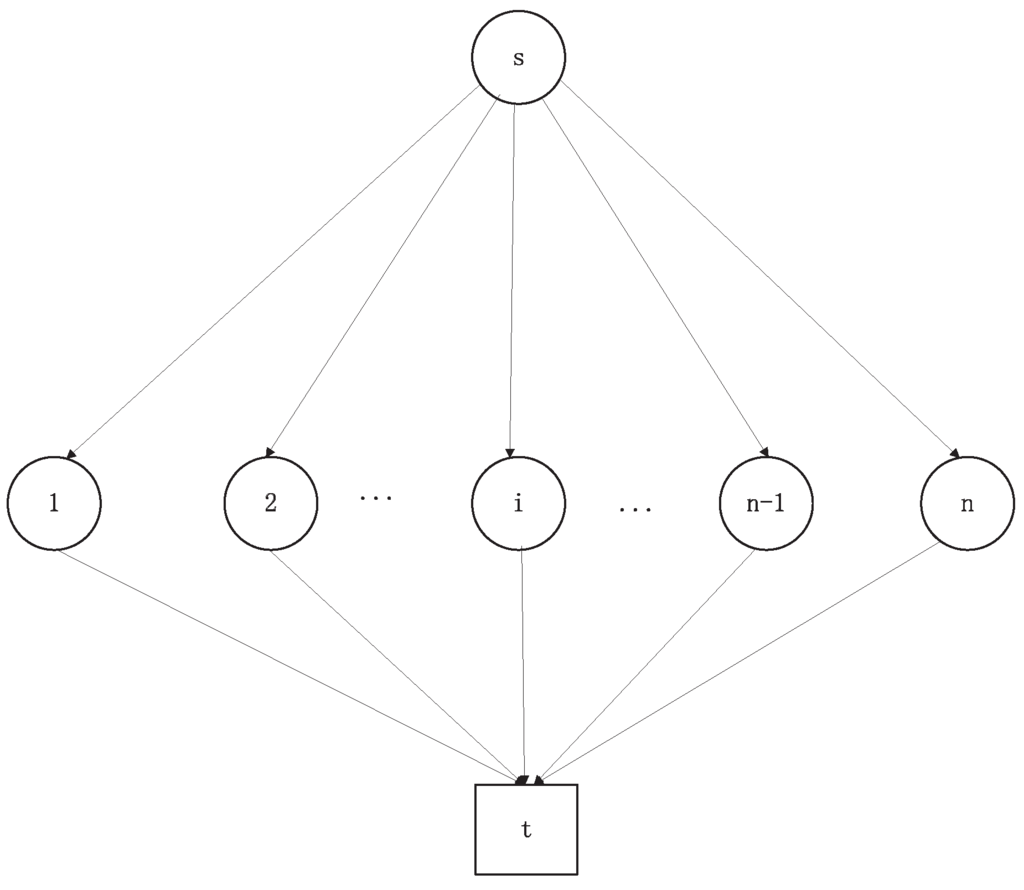
Figure 1. Treating wiretap channel II as a special case of wiretap network.

Note that since both the coding schemes developed in [5] and [6] rely on a Galois field with sufficiently large size, neither of them work on the classic wiretap channel of type II, where the symbol of each transmission is binary.

In this paper, we study a special class of wiretap network with a single source node and K sink nodes (considered as distributed servers or disk blocks), which is depicted in Figure 2. In this network model, the legitimate users are able to connect to any ${\mu }_1$ sink nodes. On the other hand, there exist eavesdroppers who are able observe digital sequences from arbitrary ${\mu }_2<{\mu }_1$ sink nodes. We propose a randomized secure network coding scheme, ensuring that every legitimate user is able to recover the source message with an arbitrarily small average decoding error probability while every eavesdropper has vanishing information about the source message. The coding scheme in this paper works over the binary field (alphabet), which indicates the complexity of the scheme does not increase accordingly with the scale of the network. Moreover, the coding scheme in this paper can work on the classic wiretap channel II readily, indicating that communication model in this paper includes wiretap channel II as a special case. Differences among the coding schemes in [5,6] and this paper are summarized in Table 1.

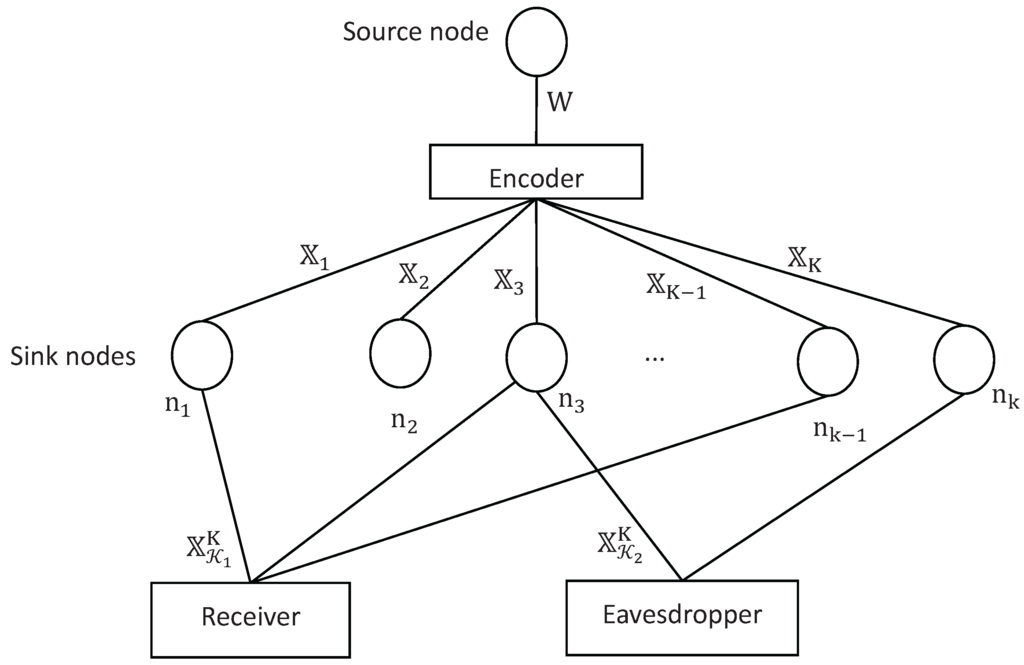
Figure 2. Communication model of wiretap network in this paper with K sink nodes.

Table 1. Comparison of different coding schemes. $P_e$ represents the averaged decoding error probability (cf. Equation (2)). Δ represents the quantity of information about source message exposed to the eavesdroppers (cf. Equation (3)). $C_s$ is the secrecy capacity (cf. Definition 5) and ϵ and τ are arbitrarily positive real values.

Coding Scheme	Reliability	Security	Transmission Rate	Field Size
introduced in [5]	$P_e=0$	$\Delta =0$	$C_s$	$\ge \left(\genfrac{}{}{0pt}{}{K}{{\mu }_2}\right)$
introduced in [6]	$P_e=0$	$\Delta =0$	$C_s-\tau$	$\ge O(|\mathcal{E}{|}^{1/\tau })$
introduced in this paper	$P_e<ϵ$	$\Delta <ϵ$	$C_s-\tau$	2 (binary)

The coding scheme in this paper comes from that of arbitrarily varying channels (AVCs). In fact, the network defined in this paper can be readily regarded as a special class arbitrarily varying wiretap channels (AVWCs) with constrained state sequences. The difference is that the receivers know the channel state sequences in our case, and hence just one single codebook is enough to assure the reliable transmission (see Remark 8 for details). The partitioning scheme is based on Csiszár’s almost independent coloring scheme [10], which has been recently used to solve the security problem of wiretap channel II with the noisy main channel [11]. Some results on the secrecy capacity of AVWCs can be found in [12,13,14].

Designing a coding scheme with a small field size is critical in some practical engineering problems. As an example, consider the situation where the transmitter needs to send a big file to the receiver through the Internet. To achieve this, the big file is divided into many data frames. Since the size of each data frame is less than 1500 bytes according to the TCP (Transmission Control Protocol) or UDP (User Datagram Protocol) protocols, the number of data frames will be quite large when the size of the file is huge. Packet loss is quite a common problem in network communication. When some data frames get lost, a common method is to require the transmitter to send the lost data frames again. Now, supposing that we plan to deal with the problem of frame loss via the coding scheme, each sink node in Figure 2 can be regarded as a data frame divided from the big file with $K=|\mathcal{E}|$ being the total number of the data frames. Since the size of each data frame is constrained, it cannot represent arbitrarily a large Galois field. Consequently, the number of K cannot be arbitrarily large when the coding schemes in [5,6] are applied, indicating that the size of the big file is constrained. However, if our coding scheme is used, the size of the big file can be arbitrary.

Another application of this model is for splitting and sharing secrete information among authorized persons. In this scenario, a group of n persons is allowed to reconstruct the secrete information correctly, while any groups with less participants can not read the split message. Please refer to [15] and references therein.

The remainder of this paper is organized as follows: the notations and problem statements are introduced in Section 2 and the main result is presented in Section 3. Furthermore, the direct and converse proofs are given in Section 4 and Section 5, respectively. Section 6 explains the coding scheme in Section 4 via two simple examples. Section 7 gives the discussions on the field size, and Section 8 concludes this paper.

2. Notations and Problem Statements

Throughout the paper, $\mathbb{N}$ is the set of positive integers and $[1:N]=\{1,2,...,N\}$ for any $N\in \mathbb{N}$.

Random variables, sample values and alphabets (sets) are denoted by capital letters, lower case letters and calligraphic letters, respectively. A similar convention is applied to random vectors and their sample values. For example, $X^N$ represents a random N-vector ($X_1,X_2,...,X_N$), and $x^N$ is a specific vector of $X^N$ in ${\mathcal{X}}^N$. ${\mathcal{X}}^N$ is the Nth Cartesian power of $\mathcal{X}$.

Let “?” be a “dummy” letter. For any index set $\mathcal{I}\subseteq [1:N]$ and finite alphabet $\mathcal{X}$ not containing the “dummy” letter “?”, denote

$${\mathcal{X}}_{\mathcal{I}}^N=\{(x_1,x_2,...,x_N):x_i\in \mathcal{X}\text{if}i\in \mathcal{I}\text{and}{x}_i=?\text{otherwise}\}.$$

For any given random vector $X^N=(X_1,X_2,...,X_N)$ and index set $\mathcal{I}\subseteq [1:N]$,

• $X_{\mathcal{I}}^N=(X_1^{\prime },X_2^{\prime },...,X_N^{\prime })$ is a “projection” of $X^N$ onto $\mathcal{I}$ with $X_n^{\prime }=X_n$ for $n\in \mathcal{I}$, and $X_n^{\prime }=?$ otherwise;
• $X_{\mathcal{I}}=(X_i,i\in \mathcal{I})$ is a subvector of $X^N$.

The random vector $X_{\mathcal{I}}^N$ takes value from ${\mathcal{X}}_{\mathcal{I}}^N$, while the random vector $X_{\mathcal{I}}$ takes value from ${\mathcal{X}}^{|\mathcal{I}|}$.

Example 1. 

Supposing that $N=5$, the index set $\mathcal{I}=\{1,3,5\}$ and the random vector $X^N=(X_1,X_2,X_3,X_4,X_5)$, we have $X_{\mathcal{I}}^N=(X_1,?,X_3,?,X_5)$ and $X_{\mathcal{I}}=(X_1,X_3,X_5)$.

Proposition 1. 

For any N-random vector $X^N$ and index set $\mathcal{I}\subseteq [1:N]$, it holds that $H(X_{\mathcal{I}}^N)=H(X_{\mathcal{I}}).$

Proof. 

Let g be a mapping from ${\mathcal{X}}_{\mathcal{I}}^N$ to ${\mathcal{X}}^{|\mathcal{I}|}$ such that

$$g(y^N)=y_{\mathcal{I}}$$

for every $y^N\in {\mathcal{X}}_{\mathcal{I}}^N$. One can easily verify that g is an one-to-one mapping. Furthermore,

$$Pr\{X_{\mathcal{I}}^N=y^N\}=Pr\{X_{\mathcal{I}}=y_{\mathcal{I}}\}=Pr\{X_{\mathcal{I}}=g(y^N)\}=\sum _{x^N\in {\mathcal{X}}^N:x_{\mathcal{I}}^N=y^N}Pr\{X^N=x^N\}$$

for every $y^N\in {\mathcal{X}}_{\mathcal{I}}^N$, implying that $X_{\mathcal{I}}^N$ and $X_{\mathcal{I}}$ share the same distribution. This completes the proof of the proposition. ☐

The communication model of wiretap network with K sink nodes, depicted in Figure 2, consists of four parts, namely encoder, network, receiver and eavesdropper. The formal definitions of those parts are introduced in Definitions 1–4, respectively. The definition of achievable transmission rate is given in Definition 5.

Definition 1. 

(Encoder) The source message W is uniformly distributed on the message set $\mathcal{W}=[1:M]$. The (stochastic) encoder is specified by a matrix of conditional probability $E(x^N|w)$ for $x^N\in {\mathcal{X}}^N$ and $w\in \mathcal{W}$, indicating the probability that the message w is encoded into the digital sequence $x^N$, where $\mathcal{X}=\{0,1\}$ is binary.

Definition 2. 

(Network) Suppose that the source message W is encoded into $X^N=(X_1,X_2,...,X_N)$. The encoder firstly divides $X^N$ into K parts, denoted by ${\mathbb{X}}_1,{\mathbb{X}}_2,...,{\mathbb{X}}_K$ with

$${\mathbb{X}}_k=(X_{(k-1)N_K+1},X_{(k-1)N_K+2},...,X_{k{N}_K})$$

for all $1\le k\le K$, where $N_K=\frac{N}{K}$ is an integer without loss of generality. Then, those sequences are transmitted to the sink nodes $n_1,n_2,...,n_K$, respectively, through K noiseless channels. Therefore, the digital sequence received by the sink node $n_k$ is ${\mathbb{X}}_k$ for every $1\le k\le K$. Let

$${\mathcal{I}}_k={\mathcal{I}}_k(N_K)=\{(k-1)N_K+1,(k-1)N_K+2,...,k{N}_K\}.$$

(1)

The sequence ${\mathbb{X}}_k$ can then be rewritten as $X_{{\mathcal{I}}_k}$.

Definition 3. 

(Receiver) Let $0<{\alpha }_1\le 1$ be a constant real number with ${\mu }_1=K{\alpha }_1$ being an integer. The receiver is able to access digital sequences from arbitrary ${\mu }_1$ sink nodes. Let

$${\mathfrak{K}}_1={\mathfrak{K}}_1(K,{\mu }_1)=\{{\mathcal{K}}_1\subseteq [1:K]:|{\mathcal{K}}_1|={\mu }_1\}$$

be the collection of subsets of sink nodes possibly selected by the receiver. The whole digital sequence obtained by the receiver may be any random sequence from $\{{\mathbb{X}}_{{\mathcal{K}}_1}^K:{\mathcal{K}}_1\in {\mathfrak{K}}_1\},$ where ${\mathbb{X}}_{{\mathcal{K}}_1}^K=X_{{\mathcal{I}}_{{\mathcal{K}}_1}}^N$ with ${\mathcal{I}}_{{\mathcal{K}}_1}={\bigcup }_{k\in {\mathcal{K}}_1}{\mathcal{I}}_k$. It is clear that $X_{{\mathcal{I}}_{{\mathcal{K}}_1}}^N$ is distributed on ${\mathcal{X}}_{{\mathcal{I}}_{{\mathcal{K}}_1}}^N$. Denoting by

$${\mathcal{X}}^N({\mathfrak{K}}_1)=\bigcup _{{\mathcal{K}}_1\in {\mathfrak{K}}_1}{\mathcal{X}}_{{\mathcal{I}}_{{\mathcal{K}}_1}}^N,$$

the decoder is a mapping $\varphi :{\mathcal{X}}^N({\mathfrak{K}}_1)\mapsto \mathcal{W}$. If it is known that the receiver has access to the sink nodes, whose indices lie in ${\mathcal{K}}_1$, the estimation of the source message is then denoted by $\widehat{W}({\mathcal{I}}_{{\mathcal{K}}_1})=\varphi (X_{{\mathcal{I}}_{{\mathcal{K}}_1}}^N)=\varphi ({\mathbb{X}}_{{\mathcal{K}}_1}^K)$, and the average decoding error probability is $Pr\{\widehat{W}({\mathcal{I}}_{{\mathcal{K}}_1})\ne W\}$. However, since the sink nodes accessed by the receiver are actually unknown, the average decoding error is defined as

$$P_e=\underset{{\mathcal{K}}_1\in {\mathfrak{K}}_1}{max}Pr\{\widehat{W}({\mathcal{I}}_{{\mathcal{K}}_1})\ne W\}.$$

(2)

Remark 1. 

Denoting ${\lambda }_1=N{\alpha }_1$, it follows that $|{\mathcal{I}}_{{\mathcal{K}}_1}|={\lambda }_1$ for every ${\mathcal{K}}_1\in {\mathfrak{K}}_1$. Consequently, setting

$${\mathfrak{I}}_{{\lambda }_1}={\mathfrak{I}}_{{\lambda }_1}(N)=\{\mathcal{I}\subseteq [1:N]:|\mathcal{I}|={\lambda }_1\}$$

yields ${\mathcal{I}}_{{\mathcal{K}}_1}\in {\mathfrak{I}}_{{\lambda }_1}$ for every ${\mathcal{K}}_1\in {\mathfrak{K}}_1$.

Remark 2. 

The communication model can also be regarded as a wiretap network with $|{\mathfrak{K}}_1|$ legitimate receivers, each of whom has access to a certain set of sink nodes in ${\mathfrak{K}}_1$. Equation (2) represents the maximal value of the average decoding error probabilities of all those legitimate receivers.

Definition 4. 

(Eavesdropper) Let $0<{\alpha }_2<{\alpha }_1$ be a constant real number with ${\mu }_2=K{\alpha }_2$ being an integer. The eavesdropper is able to access digital sequences of arbitrary ${\mu }_2$ sink nodes. Let

$${\mathfrak{K}}_2={\mathfrak{K}}_2(K,{\mu }_2)=\{{\mathcal{K}}_2\subseteq [1:K]:|{\mathcal{K}}_2|={\mu }_2\}$$

be the collection of subsets of sink nodes possibly selected by the eavesdropper. The whole digital sequence obtained by the eavesdropper may be any random sequence from $\{{\mathbb{X}}_{{\mathcal{K}}_2}^K:{\mathcal{K}}_2\in {\mathfrak{K}}_2\},$ where ${\mathbb{X}}_{{\mathcal{K}}_2}^K=X_{{\mathcal{I}}_{{\mathcal{K}}_2}}^N$ with ${\mathcal{I}}_{{\mathcal{K}}_2}={\bigcup }_{k\in {\mathcal{K}}_2}{\mathcal{I}}_k$. The quantity of source information exposed to the eavesdropper is then denoted by

$$\Delta =\underset{{\mathcal{K}}_2\in {\mathfrak{K}}_2}{max}I(W;{\mathbb{X}}_{{\mathcal{K}}_2}^K)=\underset{{\mathcal{K}}_2\in {\mathfrak{K}}_2}{max}I(W;X_{{\mathcal{I}}_{{\mathcal{K}}_2}}^N).$$

(3)

Remark 3. 

Similar to Remark 1, denoting ${\lambda }_2=N{\alpha }_2$ and

$${\mathfrak{I}}_{{\lambda }_2}={\mathfrak{I}}_{{\lambda }_2}(N)=\{\mathcal{I}\subseteq [1:N]:|\mathcal{I}|={\lambda }_2\},$$

it follows that ${\mathcal{I}}_{{\mathcal{K}}_2}\in {\mathfrak{I}}_{{\lambda }_2}$ for every ${\mathcal{K}}_2\in {\mathfrak{K}}_2$.

Remark 4. 

The communication model can also be regarded as a wiretap network with $|{\mathfrak{K}}_2|$ eavesdroppers, each of whom has access to a certain set of sink nodes in ${\mathfrak{K}}_2$. Equation (3) represents the maximal quantity of exposed source information to those eavesdroppers.

Example 2. 

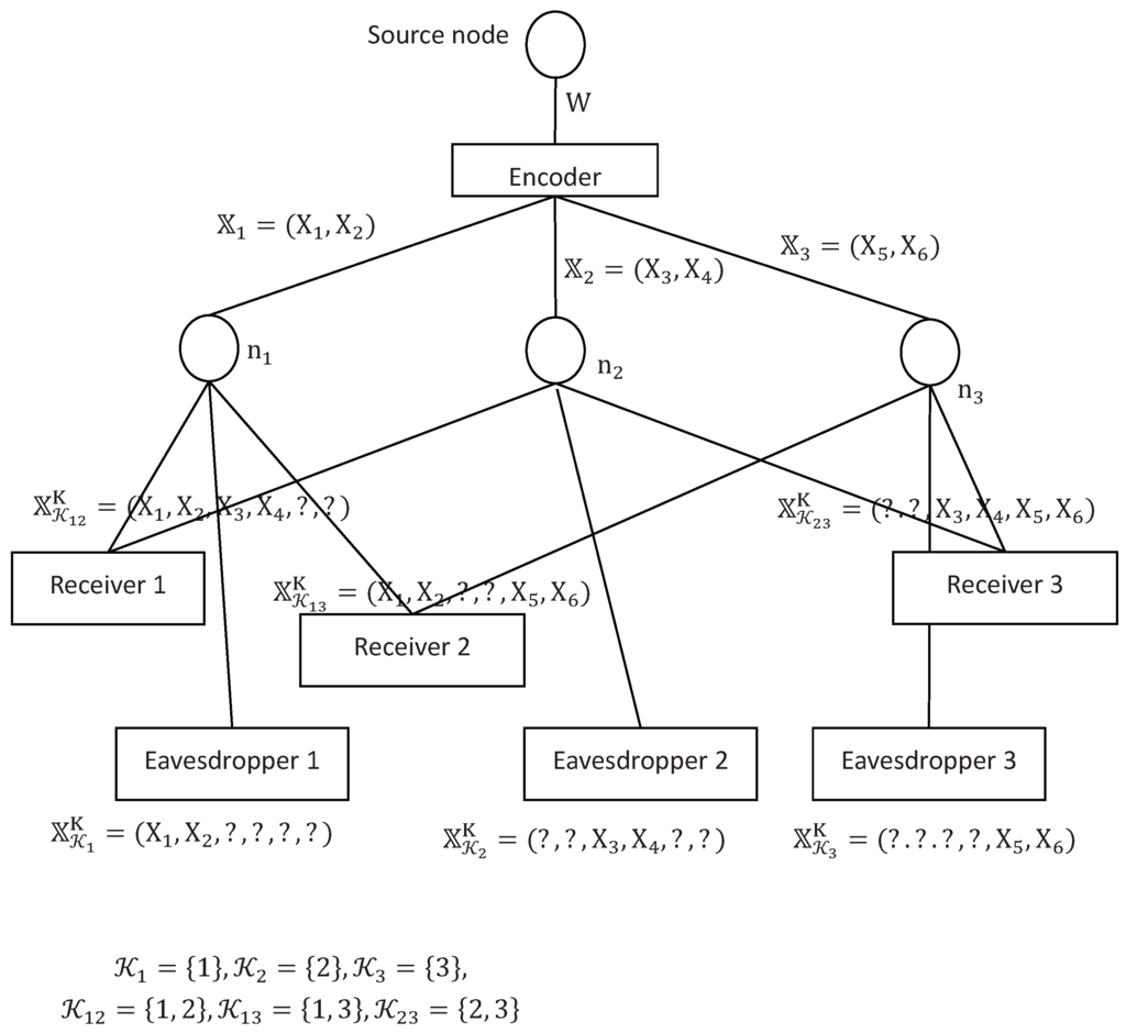
To have a clearer idea on the notations defined in this section, a special example of wiretap network is given in Figure 3 with

$$N=6,K=3,{\alpha }_1=\frac{2}{3}\text{and}{\alpha }_2=\frac{1}{3}.$$

This can be treated as a network with three receivers and three eavesdroppers. In this case, we have

$$\begin{array}{c}{\mu }_1=2,{\mu }_2=1,{\lambda }_1=4,{\lambda }_2=2,\\ {\mathcal{I}}_1=\{1,2\},{\mathcal{I}}_2=\{3,4\},{\mathcal{I}}_3=\{5,6\},\\ {\mathfrak{K}}_1=\{{\mathcal{K}}_{12},{\mathcal{K}}_{13},{\mathcal{K}}_{23}\},{\mathfrak{K}}_2=\{{\mathcal{K}}_1,{\mathcal{K}}_2,{\mathcal{K}}_3\},\\ {\mathcal{I}}_{{\mathcal{K}}_{12}}={\mathcal{I}}_1\cup {\mathcal{I}}_2=\{1,2,3,4\},{\mathcal{I}}_{{\mathcal{K}}_{13}}={\mathcal{I}}_1\cup {\mathcal{I}}_3=\{1,2,5,6\},\\ {\mathcal{I}}_{{\mathcal{K}}_{23}}={\mathcal{I}}_2\cup {\mathcal{I}}_3=\{3,4,5,6\},\\ {\mathcal{I}}_{{\mathcal{K}}_1}={\mathcal{I}}_1=\{1,2\},{\mathcal{I}}_{{\mathcal{K}}_2}={\mathcal{I}}_2=\{3,4\},{\mathcal{I}}_{{\mathcal{K}}_3}={\mathcal{I}}_3=\{5,6\},\end{array}$$

with

$${\mathcal{K}}_{12}=\{1,2\},{\mathcal{K}}_{13}=\{1,3\},{\mathcal{K}}_{23}=\{2,3\}$$

and

$${\mathcal{K}}_1=\{1\},{\mathcal{K}}_2=\{2\},{\mathcal{K}}_3=\{3\}.$$

Figure 3. An example of wiretap network II with three sink nodes.

Definition 5. 

(Achievablility) A non-negative real number R is said to be achievable, if for any $ϵ>0$ there exists an integer $N_0$ such that for any $N>N_0$, one can construct a pair of encoder and decoder $(E,\varphi )$ of length N satisfying

$$\frac{1}{N}logM>R-ϵ,$$

(4)

$$P_e<ϵ,$$

(5)

and

$$\Delta <ϵ.$$

(6)

The capacity of the communication model described in Figure 2 is denoted by $C_s$.

Remark 5. 

When regarding the communication model depicted in Figure 2 as a wiretap network with multiple legitimate receivers and multiple eavesdroppers, Equations (5) and (6) require that every legitimate receiver is able to decode the source message with a vanishing average decoding error probability, and the quantity of information about the source message exposed to every eavesdropper is vanishing.

3. The Main Result

Theorem 1. 

The capacity of the communication model of wiretap network described in Figure 2 is $C_s={\alpha }_1-{\alpha }_2$.

The direct half of Theorem 1 is given in Section 4, and the converse half is in Section 5.

The problem of wiretap network was firstly studied by Cai and Yeung in [5]. They constructed a linear network coding scheme over the wiretap network such that the legitimate receivers were able to decode the source message with exactly no decoding error while the eavesdroppers had absolutely no information on the source message. However, the coding scheme should work on a Galois field whose size was related to the scale of the network. When the number of nodes in the network increased, the size of the Galois field should have been larger accordingly, which made the encoding process much more complicated. On the other hand, the coding scheme introduced in this paper is unrelated to the scale of the network. Therefore, it turns out to be simpler than the coding scheme in [5] when the scale of the network is quite huge.

Moreover, the coding scheme in this paper is designed with a binary alphabet. Therefore, this scheme can be readily applied to the classic wiretap channel II, indicating that the communication model in this paper includes wiretap channel II as a special case. See Section 7 for details.

4. Direct Half of Theorem 1

This section gives the proof of the direct half of Theorem 1, i.e., it is achievable for every $R\le C_s={\alpha }_1-{\alpha }_2$. More precisely, we need to prove that for any $0<\tau <1,0<ϵ<1$ and any sufficiently large N, there exists a pair of encoder and decoder $(E,\varphi )$ satisfying

$$\frac{1}{N}logM=R={\alpha }_1-{\alpha }_2-\tau ,$$

(7)

$$P_e<ϵ,$$

(8)

and

$$\Delta <ϵ.$$

(9)

On account of Remarks 1 and 3, it follows that

$$P_e<P_e^{\prime }=\underset{\mathcal{I}\in {\mathfrak{I}}_{{\lambda }_1}}{max}Pr\{W\ne \widehat{W}(X_{\mathcal{I}}^N)\},$$

and

$$\Delta <{\Delta }^{\prime }=\underset{\mathcal{I}\in {\mathfrak{I}}_{{\lambda }_2}}{max}I(W;X_{\mathcal{I}}^N).$$

Therefore, instead of constructing encoder and decoder pair $(E,\varphi )$ satisfying Equations (7)–(9), this section would prove the existence of the encoder and decoder pair satisfying Equation (7),

$$P_e^{\prime }=\underset{\mathcal{I}\in {\mathfrak{I}}_{{\lambda }_1}}{max}Pr\{W\ne \widehat{W}(X_{\mathcal{I}}^N)\}<ϵ,$$

(10)

and

$${\Delta }^{\prime }=\underset{\mathcal{I}\in {\mathfrak{I}}_{{\lambda }_2}}{max}I(W;X_{\mathcal{I}}^N)<ϵ.$$

(11)

The main idea of the proof goes as follows. Let the codebook C be randomly generated, such that the size of the codebook is about $2^{N{\alpha }_1}=2^{{\lambda }_1}$. Then, partition the codebook C into about $2^{N({\alpha }_1-{\alpha }_2)}=2^{{\lambda }_1-{\lambda }_2}$ subcodes, each of which is related to a unique source message. Since the receiver is able to obtain a ${\lambda }_1$-subsequence of the transmitted codeword, which is probably distinct from those corresponding subsequences of other codewords, the receiver is able to decode the source message with a vanishing average decoding error probability. On the other hand, receiving a ${\lambda }_2$-subsequence of the transmitted codeword, the eavesdropper concludes that the transmitted codeword comes from a collection of about $2^{{\lambda }_1-{\lambda }_2}$ codewords. If those codewords are uniformly distributed on every subcode, the eavesdropper is unable to have any information on the source message.

The proof is organized as follows. Section 4.1 firstly gives the coding scheme achieving the capacity. Then, Section 4.2 establishes that, using the scheme of generating codebook randomly, we can obtain the codebook satisfying Equation (10) with probability $\to 1$ when $N\to \infty$. Finally, Section 4.3 shows that when N is sufficiently large, there exists a desired “good” partition on every random generated sample codebook such that Equation (14) holds. Equation (11) is an immediate consequence of (14) and Remark 6. Equation (7) is obtained directly from (13). Therefore, the direct half of Theorem 1 is totally established.

4.1. Code Construction

Codebook generation. Let $C={\{X^N(l)\}}_{l=1}^{M^{\prime }}$ be the ordered set of $M^{\prime }$ i.i.d. random vectors with mass function $Pr\{X^N(l)=x^N\}=\frac{1}{2^N}$ for all $1\le l\le M^{\prime }$ and $x^N\in {\mathcal{X}}^N$, where

$$M^{\prime }=2^{N({\alpha }_1-\frac{\tau }{2})}.$$

(12)

Codebook partition. Suppose that $\mathcal{C}={\{x^N(l)\}}_{l=1}^{M^{\prime }}$ is a specific sample value of $M^{\prime }$ randomly generated codewords. Let $W^{\prime }$ be a random variable uniformly distributed on $[1:M^{\prime }]$ and $X^N(\mathcal{C})=x^N(W^{\prime })$ be the random sequence uniformly distributed on $\mathcal{C}$. Set $R={\alpha }_1-{\alpha }_2-\tau$ and partition $\mathcal{C}$ into

$$M=2^{NR}=2^{N({\alpha }_1-{\alpha }_2-\tau )}$$

(13)

subsets ${\{{\mathcal{C}}_m\}}_{m=1}^M$ with equal cardinality, i.e., $|{\mathcal{C}}_m|=\frac{M^{\prime }}{M}\text{for}\text{any}1\le m\le M$. Let $\tilde{W}$ be the index of subcode containing $X^N(\mathcal{C})$, i.e., $X^N(\mathcal{C})\in {\mathcal{C}}_{\tilde{W}}$. We need to find a partition of the codebook $\mathcal{C}$ satisfying

$$\underset{\mathcal{I}\in {\mathfrak{I}}_{{\lambda }_2}}{max}I(\tilde{W};X_{\mathcal{I}}^N(\mathcal{C}))<ϵ.$$

(14)

The partition satisfying Inequality (14) is called a “good” partition. It will be proved in Section 4.3 that there exists desired “good” partition on every given sample codebook when the block length N is sufficiently large.

Encoder. Suppose that a desired partition ${\{{\mathcal{C}}_m\}}_{m=1}^M$ on a specific codebook $\mathcal{C}$ is given. When the source message W is to be transmitted, the encoder uniformly randomly chooses a codeword from the subcode ${\mathcal{C}}_W$ and emits it to the network.

Remark 6. 

For a given codebook $\mathcal{C}$ and a desired partition applied on it, denote by $X^N$ the output of the encoder, when the source message W is transmitted. It is clear that $(W,X^N)$ and $(\tilde{W},X^N(\mathcal{C}))$ share the same joint distribution.

Decoder. Suppose that a desired partition ${\{{\mathcal{C}}_m\}}_{m=1}^M$ on a deterministic codebook $\mathcal{C}={\{x^N(l)\}}_{l=1}^{M^{\prime }}$ is given. Receiving digital sequence $y^N\in {\mathcal{X}}_{\mathcal{I}}^N$ from the sink nodes, the decoder tries to find the minimal number of $\widehat{l}$ such that $x_{\mathcal{I}}^N(\widehat{l})=y^N$, and decodes $\widehat{w}$ as the estimation of the transmitted source message, where $\widehat{w}$ is the index of subcode containing $x^N(\widehat{l})$, i.e., $x^N(\widehat{l})\in {\mathcal{C}}_{\widehat{w}}$, and

$$\mathcal{I}=\mathcal{I}(y^N)=\{1\le i\le N:y_i\in \mathcal{X}\}.$$

4.2. Proof of Inequality (10)

This subsection establishes that using the coding scheme introduced in Section 4.1, one can generate a codebook satisfying Equation (10) with probability $\to 1$ when the block length $N\to \infty$.

Let $\mathcal{C}={\{x^N(l)\}}_{l=1}^{M^{\prime }}$ be a fixed codebook applied by the encoder. For any $1\le l\le M^{\prime }$ and $\mathcal{I}\in {\mathfrak{I}}_{{\lambda }_1}$, denote

$$U(\mathcal{C},l,\mathcal{I})=|\{1\le l^{\prime }<l:x_{\mathcal{I}}^N(l^{\prime })=x_{\mathcal{I}}^N(l)\}|,$$

and

$$U(\mathcal{C},\mathcal{I})=|\{1\le l\le M^{\prime }:U(\mathcal{C},l,\mathcal{I})\ge 1\}|.$$

Then, it follows from the decoding scheme introduced in Section 4.1 that

$$P_e^{\prime }=P_e^{\prime }(\mathcal{C})=\underset{\mathcal{I}\in {\mathfrak{I}}_{{\lambda }_1}}{max}\frac{U(\mathcal{C},\mathcal{I})}{M^{\prime }}.$$

(15)

Therefore, Equation (5) is finally established by the following lemma, whose proof is given in Appendix A.

Lemma 1. 

Let $C=\{X^N(1),X^N(2),...,X^N(M^{\prime })\}$ be the codebook randomly generated via the scheme introduced in Section 4.1. It holds that

$$Pr\{\underset{\mathcal{I}\in {\mathfrak{I}}_{{\lambda }_1}}{max}U(C,\mathcal{I})\le ϵM^{\prime }\}>1-{ϵ}_1,$$

(16)

where

$${ϵ}_1={exp}_2[N-(ϵ-2^{1-\frac{N\tau }{2}}loge)M^{\prime }].$$

Remark 7. 

It is clear that ${ϵ}_1\to 0$ as $N\to \infty$, which concludes from Equations (15) and (16) that we can obtain the codebook satisfying (10) with probability $\to 1$ when $N\to \infty$.

Remark 8. 

The idea of generating codebook randomly comes from the random code for AVCs, which was firstly established by Blackwell et al. [16] and further developed by Ahlswede and Wolfowitz [17] (see also Lemma 12.10 in [18]). The coding scheme for AVCs is based on the following results. Let $C=\{X^N(1),X^N(2),...,X^N(M^{\prime })\}$ be a random codebook with $\frac{1}{N}log{M}^{\prime }$ being smaller than the capacity. If the decoding scheme of maximal mutual information (MMI) is applied by the decoder, it follows that the expected average decoding error probability under each state sequence is $<ϵ$, when N is sufficiently large. To make the random coding scheme work, for each transmission, we need a separate channel sharing the exact sample value of the random codebook, which is called the common randomness (CR). However, that would occupy a large amount of bandwidth. To solve this problem, Ahlswede developed an elimination technique [19] and claimed that it sufficed to let the random codebook C be uniformly selected from a collection of $N^2$ deterministic codebooks. Moreover, if the capacity of an AVC was positive, the encoder could send the index of selected codebook before each transmission, and no extra CR was needed.

In fact, the network model in this paper can be regarded as a special case of AVCs with state sequences known at the receiver, if we ignore the participation of eavesdroppers. The capacity of the current network model is obviously positive since each receiver has access to at least one noiseless channel. Therefore, the coding scheme for AVCs works on the current network with no need of extra CR. Nevertheless, we should point out that the communication model of AVCs with state sequences known at the receiver is essentially different from the classic AVCs. In the former model, the decoder knows exactly the probability distribution of the channel input, and this would reduce the degree of difficulty on the coding scheme. In particular, it is proved in Appendix A that a single deterministic codebook is sufficient for the current network model.

4.3. Proof of the Existence of “Good” Partition for Every Given Sample Codebook

This subsection proves the existence of “good” partition satisfying Equation (14) for every codebook generated via the scheme in Section 4.1, when N is sufficiently large. The result in this subsection can establish Equation (9) immediately on account of Remark 6. Notations in Section 4.1 will continue to be used in this Subsection.

The main result of this subsection is given in the following lemma.

Lemma 2. 

For any generated sample codebook $\mathcal{C}$ of length N satisfying

$$N>\frac{64}{\tau }\mathit{\text{and}}\frac{log5(N+1)}{N}<\frac{\tau }{8},$$

there exists a partition on it such that

$$I(\tilde{W};X_{\mathcal{I}}^N(\mathcal{C}))\le 8({\alpha }_1-{\alpha }_2)N{2}^{-\frac{N\tau }{32}}$$

(17)

for all $\mathcal{I}\in {\mathfrak{I}}_{{\lambda }_2}$.

Remark 9. 

Equation (14) is finally established from the fact that the right-hand side of Equation (17) converges to 0 as $N\to \infty$.

Proof of Lemma 2.. 

The main idea of the proof is firstly pointed out here. For any $\mathcal{I}\in {\mathfrak{I}}_{{\lambda }_2}$, to satisfy $I(\tilde{W};X_{\mathcal{I}}^N(\mathcal{C}))\to 0$, we need $H(\tilde{W}|X_{\mathcal{I}}^N(\mathcal{C}))\to logM$. On account of the following obvious equality

$$H(\tilde{W}|X_{\mathcal{I}}^N(\mathcal{C}))=\sum _{z^N\in {\mathcal{X}}_{\mathcal{I}}^N}H(\tilde{W}|X_{\mathcal{I}}^N(\mathcal{C})=z^N)Pr\{X_{\mathcal{I}}^N(\mathcal{C})=z^N\},$$

it suffices to construct a partition satisfying $H(\tilde{W}|X_{\mathcal{I}}^N(\mathcal{C})=z^N)\to logM$ for almost all the $z^N\in {\mathcal{X}}_{\mathcal{I}}^N$. In the following proof, we will construct a collection of subsets $\mathcal{B}(\mathcal{C},\mathcal{I})$ of $X_{\mathcal{I}}^N$, namely Equation (21), and prove that there exists a partition on $\mathcal{C}$ such that $H(\tilde{W}|X_{\mathcal{I}}^N(\mathcal{C})=z^N)\to logM$ for all $z^N\in \mathcal{B}(\mathcal{C},\mathcal{I})$. Then $H(\tilde{W}|X_{\mathcal{I}}^N(\mathcal{C}))\to logM$ is proved on account of Equation (23).

The proof, based on Csiszár’s almost independent coloring scheme, is divided into the following three steps. Step 1 constructs a mapping $f:\mathcal{C}\mapsto [1:M]$ satisfying Equations (27) and (28) with the help of Lemma 2. Step 2 establishes Equation (29) from (28). Step 3 constructs a “good” partition satisfying Equation (14) from the mapping f with the help of Lemma 4.

Proof of Step 1. 

The following lemma plays an important role in the proof of step 1.

Lemma 3. 

(Lemma 3.1 in [20]) Let $\mathcal{P}$ be a set of distributions on $\mathcal{A}$. If there exist

$$0<\epsilon <\frac{1}{9}$$

(18)

and $l>0$, such that

$$\sum _{a:P(a)>l^{-1}}P(a)\le \epsilon$$

(19)

holds for all $P\in \mathcal{P}$, then for any positive integer,

$$k\le \frac{{ϵ}^{2}l}{3log(2|\mathcal{P}|)},$$

(20)

there exists a function $f:\mathcal{A}\mapsto [1:k]$, such that

$$\sum _{i=1}^k|P(f^{-1}(i))-\frac{1}{k}|<3\epsilon$$

holds for all $P\in \mathcal{P}$.

To apply Lemma 3, the main task is to construct the parameter $\mathcal{P}$. In our proof, each element P in $\mathcal{P}$ is a conditional probability distribution of $X^N(\mathcal{C})$ for a given $X_{\mathcal{I}}^N(\mathcal{C})=z^N$ for $z^N\in \mathcal{B}(\mathcal{C},\mathcal{I})$ and $\mathcal{I}\in {\mathfrak{I}}_{{\lambda }_2}$. The set $\mathcal{B}(\mathcal{C},\mathcal{I})$ is defined as

$$\mathcal{B}(\mathcal{C},\mathcal{I})=\{z^N\in {\mathcal{X}}_{\mathcal{I}}^N:U(\mathcal{C},z^N,\mathcal{I})>2^{N({\alpha }_1-{\alpha }_2-\frac{3\tau }{4})}\},$$

(21)

where

$$U(\mathcal{C},z^N,\mathcal{I})=|\{1\le l\le M^{\prime }:x_{\mathcal{I}}^N(l)=z^N\}|.$$

The useful properties of $\mathcal{B}(\mathcal{C},\mathcal{I})$ are given in the following proposition.

Proposition 2. 

For any $x^N\in \mathcal{C}$, $z^N\in \mathcal{B}(\mathcal{C},\mathcal{I})$ and $\mathcal{I}\in {\mathfrak{I}}_{{\lambda }_2}$, it follows that

$$Pr\{X^N(\mathcal{C})=x^N|X_{\mathcal{I}}^N(\mathcal{C})=z^N\}<2^{-N({\alpha }_1-{\alpha }_2-\frac{3\tau }{4})},$$

(22)

and

$$Pr\{X_{\mathcal{I}}^N(\mathcal{C})\notin \mathcal{B}(\mathcal{C},\mathcal{I})\}\le 2^{-\frac{N\tau }{4}}.$$

(23)

The proof of Proposition 2 will be given later in this subsection. With the help of $\mathcal{B}(\mathcal{C},\mathcal{I})$, the parameters introduced in Lemma 3 are introduced as

$$\begin{array}{c}\mathcal{A}=\mathcal{C},\\ \epsilon =2^{-\frac{N\tau }{16}},\\ l=2^{N({\alpha }_1-{\alpha }_2-\frac{3\tau }{4})},\\ k=2^{N({\alpha }_1-{\alpha }_2-\tau )},\\ \mathcal{P}=\{P_{z^N}:z^N\in \mathcal{B}(\mathcal{C},\mathcal{I}),\mathcal{I}\in {\mathfrak{I}}_{{\lambda }_2}\}\cup \{P_0\},\end{array}$$

(24)

where

$$P_0(x^N)=Pr\{X^N(\mathcal{C})=x^N\}$$

(25)

and

$$P_{z^N}(x^N)=Pr\{X^N(\mathcal{C})=x^N|X_{\mathcal{I}}^N=z^N\}.$$

(26)

The verification that parameters given in Formula (24) satisfy the requirements of Equations (18)–(20) is given in Appendix B.

Remark 10. 

Since $\mathcal{B}(\mathcal{C},\mathcal{I})\subset {\mathcal{Z}}^N$ for every $\mathcal{I}\in {\mathfrak{I}}_{{\lambda }_2}$, where $\mathcal{Z}=\mathcal{X}\cup \{?\}=\{0,1,e\}$, it follows that $|\mathcal{P}|\le |{\mathcal{Z}}^N|=3^N.$

Applying Lemma 3 with Formula (24), there exists $f:\mathcal{C}\mapsto [1:k]$ satisfying that

$$\begin{array}{ccc}{\displaystyle \sum _{i=1}^k|Pr\{X^N(\mathcal{C})\in f^{-1}(i)\}-\frac{1}{k}|}\hfill & =\hfill & {\displaystyle \sum _{i=1}^k|Pr\{W_f=i\}-\frac{1}{k}|}\hfill \\ & <\hfill & 3\epsilon \hfill \end{array}$$

(27)

and

$$\begin{array}{ccc}{\displaystyle \sum _{i=1}^k|Pr\{X^N(\mathcal{C})\in f^{-1}(i)|X_{\mathcal{I}}^N(\mathcal{C})=z^N\}-\frac{1}{k}|}\hfill & =\hfill & {\displaystyle \sum _{i=1}^k|Pr\{W_f=i|X_{\mathcal{I}}^N(\mathcal{C})=z^N\}-\frac{1}{k}|}\hfill \\ & <\hfill & 3\epsilon \hfill \end{array}$$

(28)

for all $\mathcal{I}\in {\mathfrak{I}}_{{\lambda }_2}$ and $z^N\in \mathcal{B}(\mathcal{C},\mathcal{I})$, where $W_f=f(X^N(\mathcal{C}))$.

Remark 11. 

It is clear that the function f will produce a partition on the codebook $\mathcal{C}$. Equation (27) ensures that every subcode in the partition has almost the same cardinality. Equation (28) ensures that $H(W_f|X_{\mathcal{I}}^N(\mathcal{C})=z^N)\to logk$ for $z^N\in \mathcal{B}(\mathcal{C},\mathcal{I})$.

The proof of Step 1 is completed.

Proof of Step 2. 

Set $M=k=2^{N({\alpha }_1-{\alpha }_2-\tau )}$. On account of Equation (28) and the uniformly continuity of entropy (cf. Lemma 2.7 in [18]), it follows that

$$\begin{array}{ccc}H(W_f|X_{\mathcal{I}}^N(\mathcal{C})=z^N)\hfill & \ge \hfill & logM-3\epsilon log\frac{M}{3\epsilon }\hfill \\ & \ge \hfill & logM-3N({\alpha }_1-{\alpha }_2)2^{-\frac{N\tau }{16}}\hfill \end{array}$$

for all $\mathcal{I}\in {\mathfrak{I}}_{{\lambda }_2}$ and $z^N\in \mathcal{B}(\mathcal{C},\mathcal{I})$. Combining Equation (23) and the equation above,

$$\begin{array}{ccc}H(W_f|X_{\mathcal{I}}^N(\mathcal{C}))\hfill & >\hfill & (1-2^{-\frac{N\tau }{4}})[logM-3({\alpha }_1-{\alpha }_2)N{2}^{-\frac{N\tau }{16}}]\hfill \\ & >\hfill & logM-4({\alpha }_1-{\alpha }_2)N{2}^{-\frac{N\tau }{16}},\hfill \end{array}$$

for every $\mathcal{I}\in {\mathfrak{I}}_{{\lambda }_2}$. Since $H(W_f)\le logM$, we arrive at

$$I(W_f;X_{\mathcal{I}}^N(\mathcal{C}))<4({\alpha }_1-{\alpha }_2)N{2}^{-\frac{N\tau }{16}}$$

(29)

for every $\mathcal{I}\in {\mathfrak{I}}_{{\lambda }_2}$. The proof of Step 2 is completed.

Proof of Step 3. 

The proof depends on the following lemma.

Lemma 4. 

For any given codebook $\mathcal{C}$, if the function $f:\mathcal{C}\mapsto [1:M]$ satisfies Equation (27), there exists a partition ${\{{\mathcal{C}}_m\}}_{m=1}^M$ on $\mathcal{C}$ such that

1. 

$|{\mathcal{C}}_m|=\frac{M^{\prime }}{M}$ for all $m\in [1:M]$,

2. 

$H(\tilde{W}|W_f)<4\sqrt{\epsilon }logM$,

where $\tilde{W}$ is the index of bin containing $X^N(\mathcal{C})$, i.e., $X^N(\mathcal{C})\in {\mathcal{C}}_{\tilde{W}}$.

The proof of Lemma 4 is discussed in Appendix C. In fact, Equation (27) indicates that the random variable $W_f$ is almost uniformly distributed on $[1:M]$. This implies the cardinalities of the sets $f^{-1}(i),1\le i\le M$ are quite close. Therefore, a desired partition with the same cardinality can be constructed through slight adjustments.

From Lemma 4 and Equation (29),

$$\begin{array}{ccc}I(\tilde{W};X_{\mathcal{I}}^N(\mathcal{C}))\hfill & \le \hfill & I(\tilde{W},W_f;X_{\mathcal{I}}^N(\mathcal{C}))\hfill \\ & =\hfill & I(W_f;X_{\mathcal{I}}^N(\mathcal{C}))+I(\tilde{W};X_{\mathcal{I}}^N(\mathcal{C})|W_f)\hfill \\ & \le \hfill & I(W_f;X_{\mathcal{I}}^N(\mathcal{C}))+H(\tilde{W}|W_f)\hfill \\ & \le \hfill & 4({\alpha }_1-{\alpha }_2)N{2}^{-\frac{N\tau }{16}}+4\sqrt{\epsilon }logM\hfill \\ & \le \hfill & 8({\alpha }_1-{\alpha }_2)N{2}^{-\frac{N\tau }{32}}\hfill \end{array}$$

(30)

for all $\mathcal{I}\in {\mathfrak{I}}_{{\lambda }_2}$, where M and ε are given by Equations (13) and (24), respectively. This completes the proof of Step 3.

The proof of Lemma 2 is completed. ☐

Proof of Proposition 2. 

Equation (22) follows because

$$Pr\{X^N(\mathcal{C})=x^N|X_{\mathcal{I}}^N(\mathcal{C})=z^N\}=\left\{\begin{array}{ll}\frac{1}{U(\mathcal{C},z^N,\mathcal{I})}\hfill & \text{if}{x}_{\mathcal{I}}^N=z^N,\hfill \\ 0& \text{otherwise},\end{array}\right.$$

for every $x^N\in {\mathcal{X}}^N$ and $z^N$ with $U(\mathcal{C},z^N,\mathcal{I})>0$. Equation (23) follows because

$$\begin{array}{ccc}Pr\{X_{\mathcal{I}}^N(\mathcal{C})\notin \mathcal{B}(\mathcal{C},\mathcal{I})\}\hfill & =\hfill & {\displaystyle \sum _{z^N\in {\mathcal{X}}_{\mathcal{I}}^N/\mathcal{B}(\mathcal{C},\mathcal{I})}Pr\{X_{\mathcal{I}}^N(\mathcal{C})=z^N\}}\hfill \\ & \stackrel{(a)}{=}\hfill & {\displaystyle \sum _{z^N\in {\mathcal{X}}_{\mathcal{I}}^N/\mathcal{B}(\mathcal{C},\mathcal{I})}\frac{U(\mathcal{C},z^N,\mathcal{I})}{M^{\prime }}}\hfill \\ & \stackrel{(b)}{<}\hfill & {\displaystyle \sum _{z^N\in {\mathcal{X}}_{\mathcal{I}}^N/\mathcal{B}(\mathcal{C},\mathcal{I})}{2}^{-N({\alpha }_2+\frac{\tau }{4})}}\hfill \\ & \stackrel{(c)}{\le }\hfill & 2^{-\frac{N\tau }{4}},\hfill \end{array}$$

where (a) follows from the fact that $X^N(\mathcal{C})$ is uniformly distributed on $\mathcal{C}$, (b) follows from Equation (12) and the fact that $U(\mathcal{C},z^N,\mathcal{I})<2^{N({\alpha }_1-{\alpha }_2-\frac{3\tau }{4})}$ when $z^N\notin \mathcal{B}(\mathcal{C},\mathcal{I})$ (cf. Equation (21)), and (c) follows because $|{\mathcal{X}}_{\mathcal{I}}^N|=2^{N{\alpha }_2}$. The proof of Proposition 2 is completed. ☐

5. Converse Half of Theorem 1

This section proves that every achievable rate R should be no greater than ${\alpha }_1-{\alpha }_2$, which is the converse half of Theorem 1. The proof is based on the standard technique.

Let $(E,\varphi )$ be a pair of encoder-decoder satisfying

$$\frac{1}{N}H(W)=\frac{1}{N}logM\ge R-ϵ,$$

(31)

$$P_e=\underset{{\mathcal{K}}_1\in {\mathfrak{K}}_1}{max}Pr\{\varphi (X_{{\mathcal{I}}_{{\mathcal{K}}_1}}^N)\ne W\}\le ϵ,$$

(32)

and

$$\Delta =\underset{{\mathcal{K}}_2\in {\mathfrak{K}}_2}{max}I(W;X_{{\mathcal{I}}_{{\mathcal{K}}_2}}^N)<ϵ.$$

(33)

Let ${\tilde{\mathcal{K}}}_1=[1:{\mu }_1]$ and ${\tilde{\mathcal{K}}}_2=[1:{\mu }_2]$. It follows that ${\tilde{\mathcal{K}}}_1\in {\mathfrak{K}}_1$ and ${\tilde{\mathcal{K}}}_2\in {\mathfrak{K}}_2$. Therefore, Equations (32) and (33) give

$${\tilde{P}}_e=Pr\{\varphi (X_{{\mathcal{I}}_{{\tilde{\mathcal{K}}}_1}}^N)\ne W\}\le P_e\le ϵ$$

(34)

and

$$\tilde{\Delta }=I(W;X_{{\mathcal{I}}_{{\tilde{\mathcal{K}}}_2}}^N)\le \Delta <ϵ.$$

(35)

Deduced from Equation (31), it follows that

$$\begin{array}{ccc}NR\hfill & \le \hfill & H(W)+Nϵ\hfill \\ & =\hfill & I(W;X_{{\mathcal{I}}_{{\tilde{\mathcal{K}}}_1}}^N)+H(W|X_{{\mathcal{I}}_{{\tilde{\mathcal{K}}}_1}}^N)+Nϵ\hfill \\ & \le \hfill & I(W;X_{{\mathcal{I}}_{{\tilde{\mathcal{K}}}_1}}^N)+N\delta ({\tilde{P}}_e)+Nϵ,\hfill \end{array}$$

where $\delta ({\tilde{P}}_e)\to 0$ as ${\tilde{P}}_e\to 0$ and the last inequality follows from Fano’s inequality. Combing Equation (35) and the equation above, we have

$$NR\le I(W;X_{{\mathcal{I}}_{{\tilde{\mathcal{K}}}_1}}^N)-I(W;X_{{\mathcal{I}}_{{\tilde{\mathcal{K}}}_2}}^N)+N\delta ({\tilde{P}}_e)+2Nϵ.$$

(36)

Since, clearly, $X_{{\mathcal{I}}_{{\tilde{\mathcal{K}}}_2}}^N$ is a function of $X_{{\mathcal{I}}_{{\tilde{\mathcal{K}}}_1}}^N$, we have

$$\begin{array}{ccc}I(W;X_{{\mathcal{I}}_{{\tilde{\mathcal{K}}}_1}}^N)-I(W;X_{{\mathcal{I}}_{{\tilde{\mathcal{K}}}_2}}^N)\hfill & =\hfill & I(W;X_{{\mathcal{I}}_{{\tilde{\mathcal{K}}}_1}}^N,X_{{\mathcal{I}}_{{\tilde{\mathcal{K}}}_2}}^N)-I(W;X_{{\mathcal{I}}_{{\tilde{\mathcal{K}}}_2}}^N)\hfill \\ & =\hfill & I(W;X_{{\mathcal{I}}_{{\tilde{\mathcal{K}}}_1}}^N|X_{{\mathcal{I}}_{{\tilde{\mathcal{K}}}_2}}^N)\hfill \\ & \le \hfill & H(X_{{\mathcal{I}}_{{\tilde{\mathcal{K}}}_1}}^N|X_{{\mathcal{I}}_{{\tilde{\mathcal{K}}}_2}}^N)\hfill \\ & =\hfill & H(X_{{\mathcal{I}}_{{\tilde{\mathcal{K}}}_1}/{\mathcal{I}}_{{\tilde{\mathcal{K}}}_2}}^N|X_{{\mathcal{I}}_{{\tilde{\mathcal{K}}}_2}}^N)\hfill \\ & \le \hfill & H(X_{{\mathcal{I}}_{{\tilde{\mathcal{K}}}_1}/{\mathcal{I}}_{{\tilde{\mathcal{K}}}_2}}^N).\hfill \end{array}$$

Recalling Proposition 1, the equation above is further bounded by

$$\begin{array}{ccc}I(W;X_{{\mathcal{I}}_{{\tilde{\mathcal{K}}}_1}}^N)-I(W;X_{{\mathcal{I}}_{{\tilde{\mathcal{K}}}_2}}^N)\hfill & \le \hfill & H(X_{{\mathcal{I}}_{{\tilde{\mathcal{K}}}_1}/{\mathcal{I}}_{{\tilde{\mathcal{K}}}_2}}^N)\hfill \\ & =\hfill & H(X_{{\mathcal{I}}_{{\tilde{\mathcal{K}}}_1}/{\mathcal{I}}_{{\tilde{\mathcal{K}}}_2}})\hfill \\ & \stackrel{(a)}{\le }\hfill & {\displaystyle \sum _{i\in {\mathcal{I}}_{{\tilde{\mathcal{K}}}_1}/{\mathcal{I}}_{{\tilde{\mathcal{K}}}_2}}H(X_i)}\hfill \\ & \stackrel{(b)}{\le }\hfill & |{\mathcal{I}}_{{\tilde{\mathcal{K}}}_1}/{\mathcal{I}}_{{\tilde{\mathcal{K}}}_2}|\hfill \\ & \stackrel{(c)}{=}\hfill & N({\alpha }_1-{\alpha }_2),\hfill \end{array}$$

(37)

where (a) follows from the chain rule; (b) follows because $X_i$ is binary and (c) follows because

$$|{\mathcal{I}}_{{\tilde{\mathcal{K}}}_1}/{\mathcal{I}}_{{\tilde{\mathcal{K}}}_2}|=|{\mathcal{I}}_{{\tilde{\mathcal{K}}}_1}|-|{\mathcal{I}}_{{\tilde{\mathcal{K}}}_2}|={\lambda }_1-{\lambda }_2=N({\alpha }_1-{\alpha }_2).$$

Substituting Equation (37) into (36), we arrive at

$$R<{\alpha }_1-{\alpha }_2+\delta ({\tilde{P}}_e)+2ϵ.$$

The desired inequality $R\le {\alpha }_1-{\alpha }_2$ is finally proved by letting ϵ and hence ${\tilde{P}}_e\to 0$.

6. Examples

This section gives two simple examples, showing how the coding scheme introduced in Section 4.1 works.

Example 3. 

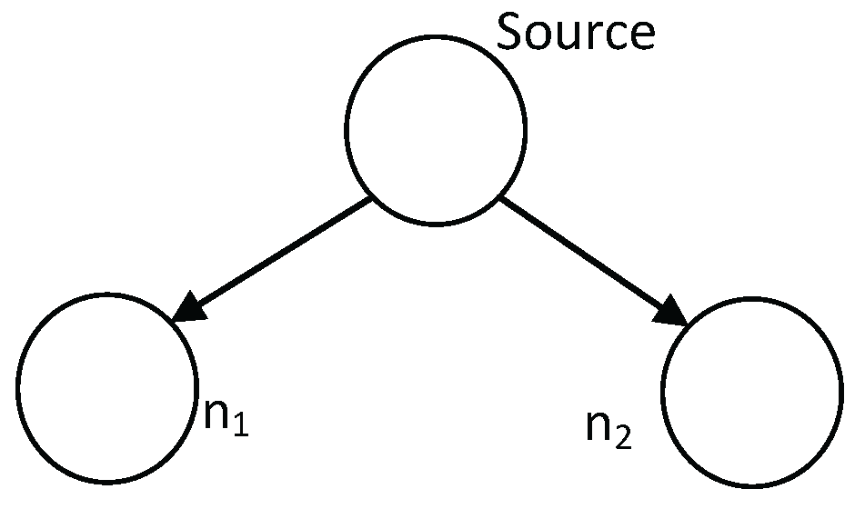
Let $N=K=2$, ${\alpha }_1=1$ and ${\alpha }_2=\frac{1}{2}$. We obtain a network with two sink nodes depicted in Figure 4. In this network, the legitimate receivers are able to access both of the sink nodes, while the eavesdroppers are able to access only one sink node. It is easy to construct a code satisfying $R=C_s={\alpha }_1-{\alpha }_2=\frac{1}{2}$, $P_e=0$ and $\Delta =0$. The coding scheme goes as the following.

• Codebook generation and partition. Let the codebook $\mathcal{C}={\{0,1\}}^2$ be partitioned as ${\mathcal{C}}_1=\{x^N(1,1)=00,x^N(1,2)=11\}$ and ${\mathcal{C}}_2=\{x^N(2,1)=01,x^N(2,2)=10\}$.
• Encoder. The source message W is uniformly distributed on the message set $\mathcal{W}=\{1,2\}$ in this example. To transmit W, a random key K, which is uniformly distributed on $\{1,2\}$ and independent of W, is firstly generated. Then, the encoder emits a codeword $x^N(W,K)$ into the network. Figure 5 shows the digital bits emitted into the sink nodes with respect to different values of W and K.
  

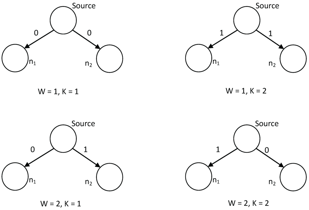  Figure 5. Coding scheme for wiretap network with two sink nodes.

Figure 4. Wiretap network with two sink nodes.

Example 4. 

Let $N=K=3$, ${\alpha }_1=\frac{2}{3}$ and ${\alpha }_2=\frac{1}{3}$. We obtain a network with three sink nodes, which is similar to that depicted in Example 2 (see also Figure 3). The only difference is that the block length $N=3$ in this example. Therefore, we have

$$\begin{array}{c}{\mathcal{I}}_{{\mathcal{K}}_i}={\mathcal{K}}_i=\{i\}\text{for}i=1,2,3,\text{and}{\mathcal{I}}_{{\mathcal{K}}_{i,j}}={\mathcal{K}}_{i,j}=\{i,j\}\text{for}(i,j)=(1,2),(1,3),(2,3).\end{array}$$

Suppose that the digital sequence emitted to the network is $X^N=(X_1,X_2,X_3)$. The digital sequences received by Receiver 1, Receiver 2 and Receiver 3 are denoted by $X_{{\mathcal{K}}_{12}}^N=(X_1,X_2,?)$, $X_{{\mathcal{K}}_{13}}^N=(X_1,?,X_3)$ and $X_{{\mathcal{K}}_{23}}^N=(?,X_2,X_3)$, respectively. The digital sequences received by Eavesdropper 1, Eavesdropper 2 and Eavesdropper 3 are denoted by $X_{{\mathcal{K}}_1}^N=(X_1,?,?)$, $X_{{\mathcal{K}}_2}^N=(?,X_2,?)$ and $X_{{\mathcal{K}}_3}^N=(?,?,X_3)$, respectively.

It can be verified by enumerating all the possible coding schems that constructing a code satisfying $R=C_s={\alpha }_1-{\alpha }_2=\frac{1}{3}$, $P_e=0$ and $\Delta =0$ is impossible for this example. A coding scheme, achieving that

$$R=\frac{1}{3},P_e=\frac{1}{4}\text{and}\Delta =\frac{6-3log3}{4},$$

is given as the following. The codebook is defined and partitioned as ${\mathcal{C}}_1=\{x^N(1,1)=000,x^N(1,2)=001\}$ and ${\mathcal{C}}_2=\{x^N(2,1)=010,x^N(2,2)=100\}$. The encoding scheme is similar to that introduced in Example 3, and hence omitted. The decoding scheme and the calculation of $P_e$ and Δ are detailed below.

Decoding scheme and calculation of $P_e$.

This part calculates the average decoding error probability of all the three receivers.

• Receiver 1. The received digital sequences of Receiver 1 with different values of W and K are given in the following table.

  W and K	Received Sequence
  W = 1, K = 1	00?
  W = 1, K = 2	00?
  W = 2, K = 1	01?
  W = 2, K = 2	10?

  The best decoding scheme is to decode sequence ’$00?$’ as $\varphi (00?)=1$, and decode the other sequences as $\varphi (01?)=\varphi (10?)=2$. The decoding error probability of Receiver 1 is $Pr\{W\ne \widehat{W}({\mathcal{I}}_{{\mathcal{K}}_{12}})\}=0$.
• Receiver 2. The received digital sequences of Receiver 2 with different values of W and K are given in the following table.

  W and K	Received Sequence
  W = 1, K = 1	0?0
  W = 1, K = 2	0?1
  W = 2, K = 1	0?0
  W = 2, K = 2	1?0

  One of the best decoding schemes is to decode sequence ’$1?0$’ as $\varphi (1?0)=2$, and decode the other sequences as $\varphi (0?0)=\varphi (0?1)=1$. In this case, a decoding error would occur when $W=2$ and $K=1$. Therefore, the average decoding error probability of Receiver 2 is $Pr\{W\ne \widehat{W}({\mathcal{I}}_{{\mathcal{K}}_{13}})\}=\frac{1}{4}$.
• Receiver 3. Similar to Receiver 2, the average decoding error probability of Receiver 3 is $Pr\{W\ne \widehat{W}({\mathcal{I}}_{{\mathcal{K}}_{23}})\}=\frac{1}{4}$.

Combing the discussions above, it is concluded that the average decoding error probability of the coding scheme is

$$P_e=max[Pr\{W\ne \widehat{W}({\mathcal{I}}_{{\mathcal{K}}_{12}})\},Pr\{W\ne \widehat{W}({\mathcal{I}}_{{\mathcal{K}}_{13}})\},Pr\{W\ne \widehat{W}({\mathcal{I}}_{{\mathcal{K}}_{23}})\}]=\frac{1}{4}.$$

Calculation of Δ.

This part calculates the amount of the source information exposed to the eavesdroppers. We only take Eavesdropper 1 as an example for the sake of simplicity. The received digital sequences with respect to different values of W and K are given in the following table.

W and K	Received Sequence
W = 1, K = 1	0??
W = 1, K = 2	0??
W = 2, K = 1	0??
W = 2, K = 2	1??

According to the table above, it follows that

$$\begin{array}{c}Pr\{X_{{\mathcal{K}}_1}^N=0??\}=\frac{3}{4},Pr\{X_{{\mathcal{K}}_1}^N=1??\}=\frac{1}{4},\\ Pr\{X_{{\mathcal{K}}_1}^N=0??|W=1\}=1,Pr\{X_{{\mathcal{K}}_1}^N=1??|W=1\}=0,\\ \text{and}Pr\{X_{{\mathcal{K}}_1}^N=0??|W=2\}=Pr\{X_{{\mathcal{K}}_1}^N=1??|W=2\}=\frac{1}{2}.\end{array}$$

This indicates that

$$\begin{array}{ccc}I(W;X_{{\mathcal{K}}_1}^N)\hfill & =\hfill & H(X_{{\mathcal{K}}_1}^N)-H(X_{{\mathcal{K}}_1}^N|W)\hfill \\ & =\hfill & H(X_{{\mathcal{K}}_1}^N)-\frac{1}{2}H(X_{{\mathcal{K}}_1}^N|W=1)-\frac{1}{2}H(X_{{\mathcal{K}}_1}^N|W=2)\hfill \\ & =\hfill & h(\frac{1}{4})-\frac{1}{2}h(0)-\frac{1}{2}h(\frac{1}{2})=\frac{6-3log3}{4}.\hfill \end{array}$$

Moreover, it can be obtained similarly that

$$I(W;X_{{\mathcal{K}}_2}^N)=I(W;X_{{\mathcal{K}}_3}^N)=\frac{6-3log3}{4}.$$

Therefore, we conclude that

$$\Delta =max[I(W;X_{{\mathcal{K}}_1}^N),I(W;X_{{\mathcal{K}}_2}^N),I(W;X_{{\mathcal{K}}_3}^N)]=\frac{6-3log3}{4}.$$

Remark 12. 

One may find that the eavesdroppers can also decode the source message with the average decoding error probability $=\frac{1}{4}$ in Example 4. This indicates that the eavesdroppers have the same decoding ability as Receiver 1 and Receiver 2. The coding scheme is not a desired one. In fact, a sufficiently large block length N is necessary to design a desired coding scheme. The examples in this section do not focus on the construction of optimal coding scheme. They just show the encoding and decoding processes when the codebook is given.

7. Discussions on Field Size

In [5], Cai and Yeung have constructed an admissible linear block code over a more general wiretap network with intermediate nodes. However, the construction was working on $GF(q)$ with q being sufficiently large. Applying coding scheme in [5] to the wiretap network of this paper, we get the following linear network encoder and decoder:

• The source message W is uniformly distributed on the message set $\mathcal{W}$ of size M;
• The stochastic encoder $\tilde{E}$ is a matrix of conditional probability $E({\tilde{x}}^k|w)$ for ${\tilde{x}}^K\in {\tilde{\mathcal{X}}}^K$ and $w\in \mathcal{W}$, indicating the probability that the message w is encoded into the digital sequence ${\tilde{x}}^K$, where $\tilde{\mathcal{X}}$ is actually the $GF(q)$. Supposing that the source message W is encoded into ${\tilde{X}}^K=({\tilde{X}}_1,{\tilde{X}}_2,...,{\tilde{X}}_K)$, the encoder emits the random symbol ${\tilde{X}}_k$ to the sink node $n_k$;
• For every ${\mathcal{K}}_1\in {\mathfrak{K}}_1$, the decoder ${\tilde{\varphi }}_{{\mathcal{K}}_1}$ is a mapping from ${\tilde{\mathcal{X}}}^{{\mu }_1}$ to $\mathcal{W}$, where ${\mu }_1=N{\alpha }_1$ (see Definition 3);
• The decoding error probability is defined as

  $${\tilde{P}}_e=\underset{{\mathcal{K}}_1\in {\mathfrak{K}}_1}{max}Pr\{{\tilde{\varphi }}_{{\mathcal{K}}_1}({\tilde{X}}_k,k\in {\mathcal{K}}_1)\ne W\},$$

  (38)

  and the quantity of source information exposed to the eavesdroppers is defined as

  $$\tilde{\Delta }=\underset{{\mathcal{K}}_2\in {\mathfrak{K}}_2}{max}I(W;{\tilde{X}}_{{\mathcal{K}}_2}^K).$$

  (39)

Remark 13. 

The decoding error probability and the quantity of exposed information formulated in Equations (38) and (39), respectively, are similar to those formulated in Equations (2) and (3), except that ${\mathbb{X}}_k$ is distributed on ${\mathcal{X}}^{N_K}$ while ${\tilde{X}}_k$ is distributed on $\tilde{\mathcal{X}}$, where $\mathcal{X}$ is binary, $\tilde{\mathcal{X}}$ is $GF(q)$ and $N_K=\frac{N}{K}$.

Remark 14. 

The coding scheme constructed above is called linear, because the encoder $\tilde{E}$ can be interpreted as a generating matrix from $G{F}^{{\mu }_1\times K}(q)$. Please refer to [5] for more details.

The following theorem is actually a direct consequence of Theorem 3 in [5].

Theorem 2. 

Suppose that the wiretap network depicted in Figure 2 with K sink nodes is given. Let $\tilde{\mathcal{X}}$ be a alphabet of size q such that

$$q=|\tilde{\mathcal{X}}|\ge max\left\{\left(\genfrac{}{}{0pt}{}{K}{{\mu }_1}\right),\left(\genfrac{}{}{0pt}{}{K}{{\mu }_2}\right)\right\},$$

(40)

with ${\mu }_1=K{\alpha }_1$ and ${\mu }_2=K{\alpha }_2$ for fixed $0\le {\alpha }_1<{\alpha }_2\le 1$ (cf. Definitions 1 and 3). Then, there exists a pair of linear block encoder $\tilde{E}$ and decoder $({\tilde{\varphi }}_{{\mathcal{K}}_1},{\mathcal{K}}_1\in {\mathfrak{K}}_1)$ working on the alphabet $\tilde{\mathcal{X}}$ such that

$$\frac{logM}{\lfloor Klogq\rfloor }={\alpha }_1-{\alpha }_2,{\tilde{P}}_e=0\text{and}\tilde{\Delta }=0,$$

(41)

where ${\tilde{P}}_e$ and $\tilde{\Delta }$ are given by Equations (38) and (39), respectively.

Theorem 2 asserts that the capacity ${\alpha }_1-{\alpha }_2$ is able to be achieved absolutely with exactly no decoding error and no exposed source information, if the alphabet is sufficiently large. However, it is well known that the alphabets of most channels are binary. To make the theorem work on the binary channels, it is necessary to map the elements in $GF(q)$ on to binary digital sequences, which produces the following corollary.

Corollary 1. 

When $N\ge Klogq$ with q satisfying Equation (40), there exists a pair of encoder-decoder $(E,\varphi )$ formulated by Definitions 1 and 3 (working on binary alphabet), such that

$$\frac{logM}{N}={\alpha }_1-{\alpha }_2,P_e=0\text{and}\Delta =0,$$

(42)

where $P_e$ and Δ are given by Equations (2) and (3), respectively.

Proof. 

Let $\tilde{E}$ and $({\tilde{\varphi }}_{{\mathcal{K}}_1},{\mathcal{K}}_1\in {\mathfrak{K}}_1)$ be a pair of linear network code working on the alphabet $\tilde{\mathcal{X}}=GF(q)$ such that Equation (41) holds, where q satisfies Equation (40). Denote $N_K=\lceil logq\rceil$. It is easy to construct an injection $f:\tilde{\mathcal{X}}\mapsto {\mathcal{X}}^{N_K}$.

Set $N=K{N}_K$. The stochastic encoder E is defined as

$$E(x^N|w)=\tilde{E}(f^{-1}(x_{{\mathcal{I}}_1}),f^{-1}(x_{{\mathcal{I}}_1}),...,f^{-1}(x_{{\mathcal{I}}_K})|w)$$

for every $x^N\in {(f(\tilde{\mathcal{X}}))}^K$ and $w\in \mathcal{W}$, where ${\mathcal{I}}_k$ is given by Equation (1) for $1\le k\le K$ and the range $f(\tilde{\mathcal{X}})$ is the subset of ${\mathcal{X}}^{N_K}$. The decoder ϕ is defined as

$$\varphi (x_{{\mathcal{I}}_{{\mathcal{K}}_1}}^N)={\tilde{\varphi }}_{{\mathcal{K}}_1}(f^{-1}(x_{{\mathcal{I}}_k}),k\in {\mathcal{K}}_1)$$

for every $x^N\in {(f(\tilde{\mathcal{X}}))}^K$ and ${\mathcal{K}}_1\in {\mathfrak{K}}_1$. One can easily verify that the pair of encoder and decoder $(E,\varphi )$ constructed above satisfies Equation (42). The proof is completed. ☐

Remark 15. 

Corollary 1 requires the block length N should satisfy that

$$N\ge Klogq\ge Kmax\{log\left(\genfrac{}{}{0pt}{}{K}{K{\alpha }_1}\right),log\left(\genfrac{}{}{0pt}{}{K}{K{\alpha }_2}\right)\}\ge K^{2}max\{h({\alpha }_1),h({\alpha }_2)\}-2Klog(K+1),$$

indicating N is an approximately quadratic function of K, where the second inequality follows from (40) and the third inequality follows from Lemma 2.3 in [18].

Remark 16. 

Through a similar way of establishing Corollary 1, it is concluded that with the coding scheme introduced in [6], for any $0<\tau <{\alpha }_1-{\alpha }_2$ and $N>O(\frac{KlogK}{\tau })$, there exists a pair of encoder-decoder $(E,\varphi )$ formulated by Definitions 1 and 3 (with binary alphabet), such that

$$\frac{logM}{N}={\alpha }_1-{\alpha }_2-\tau ,P_e=0\text{and}\Delta =0,$$

where $P_e$ and Δ are given by Equations (2) and (3), respectively.

Remark 15 claims that the block length N is an approximately quadratic function of K if the linear network coding scheme introduced in [5] is applied over the wiretap network and one needs to emit about $K·max\{h({\alpha }_1),h({\alpha }_2)\}$ digital bits onto each edge. Remark 16 asserts that by sacrificing a small portion of transmission rate, the length of digital bits emitted on each edge can be decreased to $O(\frac{logK}{\tau })$, if the coding scheme in [6] is applied. Nevertheless, when the number K of sink nodes is large, both of the encoding processes turn out to be quite complicated. To have a comparison between the coding scheme in this paper and those in [5,6], the following corollary claims that by sacrificing a tiny portion of transmission rate, it is possible to construct a pair of encoder and decoder with a vanishing average decoding error probability and vanishing exposed source information to the eavesdroppers such that only one digital bit is transmitted onto each edge when the number K of sink nodes is sufficiently large.

Corollary 2. 

For any given $0<ϵ<1$ and $0<\tau <{\alpha }_1-{\alpha }_2$, if the block length N satisfies

$$N\ge K,$$

(43)

$$N<(ϵ-2^{1-\frac{N\tau }{2}}loge)2^{N({\alpha }_1-\frac{\tau }{4})},$$

(44)

$$N>\frac{64}{\tau },$$

(45)

$$\frac{log5(N+1)}{N}<\frac{\tau }{8},$$

(46)

and

$$8({\alpha }_1-{\alpha }_2)N{2}^{-\frac{N\tau }{32}}<ϵ,$$

(47)

one can construct a pair of encoder and decoder $(E,\varphi )$ formulated by Definitions 1 and 3 (with binary alphabet), such that

$$\frac{logM}{N}\ge {\alpha }_1-{\alpha }_2-\tau ,P_e<ϵ\mathit{\text{and}}\Delta <ϵ.$$

Proof. 

On account of Lemma 1, Equation (44) claims the existence of codebook $\mathcal{C}$ with $P_e=P_e(\mathcal{C})<ϵ$. Invoking Lemma 2, Equations (45) and (46) indicate the existence of partition on the codebook $\mathcal{C}$ satisfying Equation (17). The inequality $\Delta <ϵ$ is established from Equations (17), (47) and Remark 6. The corollary is proved. ☐

Remark 17. 

The constraints (44)–(47) are independent of K. Therefore, when K is sufficiently large, only Inequality (43) is active. This indicates that we can set $N=K$, and hence it suffices to emit only one digital bit to each edge, when the number K of sink nodes is sufficiently large.

When $N=K$ and ${\alpha }_1=1$, the wiretap network depicted in Figure 2 is equivalent to the wiretap channel II [9] of N times of transmission. Each edge in the network is related to one time of transmission in wiretap channel II. See Figure 1. Therefore, the coding scheme introduced in this paper also works for the communication model of wiretap channel II. However, it is clear that the coding schemes introduced in [5,6], which depend on the size of alphabet, do not work for wiretap channel II.

After the discussion above, it has been known that the major advantage of the coding scheme in this paper is that there exists a pair of encoder and decoder such that the source message is transmitted to the legitimate receivers with exactly one time of transmission, when the number K of sink nodes is sufficiently large. More precisely, denoting by $N^{*}=N^{*}({\alpha }_1,{\alpha }_2,\tau ,ϵ)$ the minimal value of N satisfying Equations (44)–(47), when ${\alpha }_1,{\alpha }_2,\tau$ and ϵ are given, the number sink nodes K should be at least $N^{*}$ to implement the one-time transmission. The values of $N^{*}$ versus ${\alpha }_1$ and ${\alpha }_2$ is given by Figure 6. The figure shows that when $\tau =\frac{{\alpha }_1-{\alpha }_2}{10}$, the value of $N^{*}$ is totally determined by the value of ${\alpha }_1-{\alpha }_2$. As a concrete example, the data points marked in Figure 6 are those with ${\alpha }_1-{\alpha }_2=0.1$ and they lie on the identical horizontal line and hence share the same value of $N^{*}$.

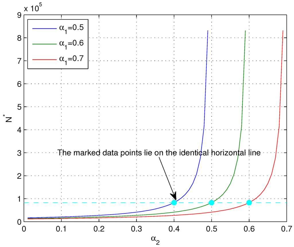
Figure 6. Values of $N^{*}$ versus ${\alpha }_1$ and ${\alpha }_2$ with $\tau =\frac{{\alpha }_1-{\alpha }_2}{10}$ and $ϵ=0.001$.

8. Conclusions

This paper constructs a secure coding scheme for a special class of network with one single source node and K sink nodes, and determines its strong secrecy capacity. Unlike the linear network coding schemes developed in [5,6], which rely on Galois fields with sufficiently large sizes, the coding scheme introduced in this paper is working on the binary alphabet and hence can be readily applied to the classic wiretap channel II.

References

- Alshwede, R.; Cai, N.; Li, S.Y.R.; Yeung, R.W. Network information flow. IEEE Trans. Inf. Theory 2000, 46, 1204–1216. [Google Scholar] [CrossRef]
- Li, S.Y.R.; Yeung, R.W.; Cai, N. Linear network coding. IEEE Trans. Inf. Theory 2003, 49, 371–381. [Google Scholar] [CrossRef]
- Ho, T.; Médard, M.; Koetter, R.; Karger, D.R.; Effros, M.; Shi, J.; Leong, B. A random linear network coding approach to multicast. IEEE Trans. Inf. Theory 2006, 52, 4413–4430. [Google Scholar] [CrossRef]
- Cai, N.; Yeung, R.W. Secure network coding. In Proceedings of the 2002 IEEE International Symposium on Information Theory, Lausanne, Switzerland, 30 June–5 July 2002.
- Cai, N.; Yeung, R.W. Secure network coding on a wiretap network. IEEE Trans. Inf. Theory 2011, 57, 424–435. [Google Scholar]
- Feldman, J.; Malkin, T.; Stein, C.; Servedio, R.A. On the capacity of secure network coding. In Proceedings of the 42nd Annual Allerton Conference on Communication, Control, and Computing, Monticello, IL, USA, 29 September–1 October 2004.
- Bhattad, K.; Narayanan, K.R. Weakly secure network coding. In Proceedings of the First Workshop on Network Coding, Theory, and Applications, Riva del Garda, Italy, 7 April 2005.
- Ho, T.; Leong, B.; Koetter, R.; Médard, M.; Effros, M.; Karger, D.R. Byzantine modification detection in multicast networks using randomized network coding. In Proceedings of the IEEE International Symposium on Information Theory, Chicago, IL, USA, 27 June–2 July 2004.
- Ozarow, L.H.; Wyner, A.D. Wire-tap channel II. AT&T Bell Lab. Tech. J. 1984, 63, 2135–2157. [Google Scholar]
- Csiszár, I. Almost independence and secrecy capacity. Prob. Inf. Transm. 1996, 32, 40–47. [Google Scholar]
- He, D.; Luo, Y.; Cai, N. Strong secrecy capacity of the wiretap channel II with DMC main channel. In Proceedings of the IEEE International Symposium on Information Theory, Barcelona, Spain, 10–15 July 2016.
- MolavianJazi, E.; Bloch, M.; Laneman, J.N. Arbitrary jamming can preclude secure communication. In Proceedings of the 47th Annual Allerton Conference on Communication, Control, and Computing, Monticello, IL, USA, 30 September–2 October 2009; pp. 1069–1075.
- Bjelaković, I.; Boche, H.; Sommerfeld, J. Capacity results for arbitrarily varying wiretap channel. In Information Theory, Combinatorics, and Search Theory; Springer: Berlin, Germany, 2013; Volume 7777, pp. 123–144. [Google Scholar]
- Boche, H.; Schaefer, R.F. Capacity results and super-activation for wiretap channels with active wiretappers. IEEE Trans. Inf. Forensics Secur. 2013, 8, 1482–1496. [Google Scholar] [CrossRef]
- Ogiela, M.R.; Ogiela, U. Linguistic approach to crypotographic data sharing. In Proceedings of the 2008 Second International Conference on Future Generation Communication and Networking, Hainan Island, China, 13–15 December 2008.
- Blackwell, D.; Breiman, L.; Thomasian, A.J. The capacities of certain channel classes under random coding. Ann. Math. Stat. 1960, 31, 558–567. [Google Scholar] [CrossRef]
- Ahlswede, R.; Wolfowitz, J. Correlated decoding for channels with arbitrarily varying channel probability functions. Inf. Control 1969, 14, 457–473. [Google Scholar] [CrossRef]
- Csiszár, I.; Körner, J. Information Theory: Coding Theorems for Discrete Memoryless Systems; Cambridge University Press: Cambridge, UK, 2011. [Google Scholar]
- Ahlswede, R. Elimination of correlation in random codes for arbitrarily varying channels. Probab. Theory Relat. Fields 1978, 44, 159–175. [Google Scholar] [CrossRef]
- Ahlswede, R.; Csiszár, I. Common randomness in information theory and cryptography—Part II: CR capacity. IEEE Trans. Inf. Theory 1998, 44, 225–240. [Google Scholar] [CrossRef]
© 2016 by the authors; licensee MDPI, Basel, Switzerland. This article is an open access article distributed under the terms and conditions of the Creative Commons Attribution (CC-BY) license (http://creativecommons.org/licenses/by/4.0/).