Abstract
In many case-control genetic association studies, a secondary phenotype that may have common genetic factors with disease status can be identified. When information on the secondary phenotype is available only for the case group due to cost and different data sources, a fitting linear regression model ignoring supplementary phenotype data may provide limited knowledge regarding genetic association. We set up a joint model and use a Bayesian framework to estimate and test the effect of genetic covariates on disease status considering the secondary phenotype as an instrumental variable. The application of our proposed procedure is demonstrated through the rheumatoid arthritis data provided by the 16th Genetic Analysis Workshop.
1. Introduction
Statistical analysis with regression models is a common approach for investigating the effects of genetic and non-genetic covariates on a response outcome. Observations in such a study usually involve a pre-specified disease trait, which could be either a continuous or categorical variable, genetic markers, such as single nucleotide polymorphisms (SNPs), candidate genes and non-genetic covariates of interest, such as age, ethnicity and environmental exposure. When the disease trait is obtained as a continuous outcome variable, linear regression models are commonly used [1,2], whereas logistic regression models, the Cochran–Armitage trend test and Pearson’s chi-squared test are often used for the analysis of a binary disease trait [3,4]. In addition, the effects of genes (SNPs) and covariates on the selected disease trait are often described through a multivariate linear or generalized linear model. Through a set of latent biological phenotypes, Chatterjee et al. [5] described a conceptual framework for modeling genetic associations and gene-gene and gene-environment interactions in indirect-association studies with multivariate logistic regression models. Maity et al. [6] extended the approaches proposed by Chatterjee et al. [5] to studies with repeated measures data and developed a class of score tests in general semi-parametric regression models. Genetic studies may also involve combined data from several case-control studies [7].
Recently, Wu et al. [8] proposed a joint regression model based on a two-step conditional modeling approach. First, they modeled the effects of SNPs and non-genetic covariates on the conditional probabilities for the categorical variable using a generalized linear model; second, based on conditioning of the given levels of a categorical variable, they modeled the added effects of the same SNPs and covariates on the conditional means of the continuous outcome using a general linear regression model. However, they modeled the conditional mean of the continuous outcome for given case and control groups separately; thus, their joint likelihood would not allow for the estimation of the effect of covariates on the continuous outcome measure in the control group when the continuous outcomes are missing in the control group. Furthermore, He et al. [9] proposed a Gaussian copula-based approach that could model the dependence between disease status and secondary phenotypes.
As progress in computational power has been extended to genetic association studies, recent studies have demonstrated the practical and theoretical advantages of using Bayesian approaches for the assessment of associations [10]. Bayesian methods compute measures of evidence that can be directly compared among SNPs within and across studies. In genome-wide association studies (GWAS), the Bayes factor is a useful tool to support significant p-values and serves as a better measure than p-values when results are compared across studies with different sample sizes. Xu et al. [11] proposed a Bayes factor based on the Cochran–Armitage trend test that incorporates situations of Hardy–Weinberg disequilibrium.
In this paper, we propose an instrumental regression model and develop a Bayesian estimation and testing procedure involving the shared genetic associations with both continuous and binary outcomes. We construct a joint-likelihood model for disease status and the continuous secondary phenotype available for the case group. In particular, we incorporate the secondary phenotype as an instrumental variable into the model and make use of the fact that the missing secondary phenotypes are known to be larger (or smaller) for the control group than for the case group. This is not an unreasonable assumption in practice, since the available phenotype is regarded as an important surrogate clinical measurement in deciding the disease status. Under various genetic models, estimation of the genetic associations and covariate effects are obtained by the Bayesian method.
For the main results, we describe the real data and data structure in Section 2 and Section 3, respectively. We describe our model and the hypotheses to be tested in Section 4 and then explain the Bayesian methodology and the corresponding testing procedures in Section 5. In Section 6, we present the application of our method to the Genetic Analysis Workshop 16 (GAW16) rheumatoid arthritis (RA) dataset. In Section 7, we provide concluding remarks with a brief discussion of the advantages and limitations of our approach.
2. RA Genetic Data
Our example comes from a GWAS exploring the effect of genetic markers on certain diseases. GWAS has emerged as an effective tool to identify a common polymorphism underlying complex diseases, and the GAW16 RA data represent the initial batch of GWAS data from the North American Rheumatoid Arthritis Consortium after removing duplicated and contaminated samples [12].
RA is a chronic inflammatory disease characterized by the destruction of the synovial joints, resulting in severe disability, particularly in patients who remain refractory to available therapies. The susceptibility to and severity of RA are determined by both genetic and environmental factors [13]. A newly-identified autoantibody, anti-cyclic citrullinated peptide (anti-CCP), appears to be highly specific for the disease and is a good predictor of erosive outcome [14]; elevations of anti-CCP have been reported to predict increased risk for development of RA [15]. RA affection is a dichotomous variable representing disease status, and anti-CCP level is a continuous trait. Moreover, information of the gender of each patient is available as an independent covariate.
The GAW16 RA data are derived from a case-control study involving 868 RA-positive patients (cases) and 1194 subjects from the New York Cancer Project, who were RA negative (controls), and the dataset contains genotype data for more than 500,000 SNPs. Since anti-CCP antibodies are potentially important surrogate markers for the diagnosis and prognosis of RA and larger anti-CCP values have been linked to increased severity of RA [14], the GAW16 data contain anti-CCP measurements for the RA-positive patients, but not for the RA-negative subjects.
For the purpose of illustration, we here present the results for a few selected SNPs on chromosome 1. Among susceptibility genes on chromosome 1, PTPN22 has been shown to be associated with RA [16], and PADI4 has been identified to be associated with RA among Asians [17]. Alleles at the PTPN22 locus have been shown to confer an increased risk for RA [18]. In particular, they reported that the R620W allele in SNP rs2476601 confers a 1.7-fold to 1.9-fold increased risk of RA to heterozygotes and even higher risks to homozygous carriers.
After removing the SNPs that were excluded using standard GWAS quality-control procedures, we obtained 34,195 SNPs on chromosome 1. Due to the skewness of the anti-CCP distribution, we used the log-transformed anti-CCP values. For preliminary analysis, we screened each individual SNP based on the results of logistic regression of RA status under an additive genetic model and selected SNPs whose p-values were smaller than (Bonferroni-corrected significance level). In Table 1, we have tabulated the top 13 ranked SNPs that were screened from the preliminary logistic analysis.

Table 1.
The 13 most significant single nucleotide polymorphisms (SNPs) from the logistic regression of rheumatoid arthritis status under the additive model.
3. Data Structure
We consider the example of genetic association studies based on a case-control sample. Let be the random variables for the traits, genetic markers and covariates being considered, where D is a binary random variable indicating a certain disease or clinical status; W is the actual value of the secondary phenotype, ; is a vector of categorical variables denoting the presence of genetic markers or SNPs; and is an -valued covariate matrix for some . Although is generally a categorical variable, specific choices for depend on whether the biallelic genetic model is recessive, additive or dominant. In practice, we identify a group of case subjects and select a certain number of control subjects matched with respect to other important characteristics, such as gender or age. Suppose that the data consist of n independent and identically distributed realizations of , where the observation for the i-th case subject is denoted by and the observation for the j-th control subject is denoted by . Although s are observed for all subjects , because of cost considerations or a situation in which the secondary phenotype W in the control group may not have an important impact on the scientific objectives of the study, may not be measured in the control group. For instance, in our example, it is well known that high anti-CCP values are associated with RA, and these values were measured for the case subjects. However, control group data were obtained from a different source, i.e., the New York Cancer Project, and therefore, the anti-CCP values are missing for the control subjects. On the other hand, the secondary phenotype serves as an important surrogate measurement for disease status; therefore, we may assume that there is a certain ordering in magnitude of the secondary phenotype values between the case group and the control group. Throughout this paper, we assume known information that W’s in the control group are smaller than those in the case group. The opposite situation can be easily dealt with by taking negative values of the secondary phenotype outcomes.
4. Model and Hypothesis
We consider two response outcomes, namely the binary disease status D and the continuous secondary phenotype outcome W. In a classical logistic regression setup, the probability of having a disease is determined by the covariates in the model. Here, we also evaluate the values of a continuous secondary phenotype, which are used as a surrogate measure to determine the disease status. The secondary phenotype W is deemed to be correlated with the disease status D and is also explained by the covariates and . Our approach relies on being able to identify a genetic variant (SNP) that perturbs the secondary phenotype, which is measured with a random error parameter. We assume that the genetic markers, as well as other non-genetic covariates, have some effect on the secondary phenotype, which serves as an intermediate outcome that, in turn, affects the disease status. For instance, because elevated anti-CCP antibody levels are associated with an increased risk of RA, we assume that this relationship may be causal. Therefore, we investigated the effect of covariates on RA status via their effect on the anti-CCP measurements as a secondary outcome. This leads to the path diagram illustrated as follows.
[Association diagram among variables]
We consider a joint regression model for with covariates constructed by modeling the conditional probability and the conditional mean of , given . Using a logit model for the binary variable and a linear model for the continuous secondary phenotype , a generalized linear joint model is given as the following hierarchical model based on and :
where . , describe the genetic association of and the covariate effect of on the probability of having the disease, respectively. describes the effect of the secondary phenotype on the disease status. and describe the genetic association of and the covariate effect of on the secondary phenotype W, and is the mean zero random error with variance . is the indicator function of a set A, and the superscript denotes the transpose of a vector or a matrix. For each genetic marker, the covariate G is a variable that depends on the assumed genetic model. Depending on the number of copies of the mutant allele at a particular SNP, we have for a dominant genetic model, for a recessive genetic model and for an additive genetic model [19]. Note that a conditional approach can be directly connected to Gibbs sampling in view of the relationship between the conditional distribution and joint distribution. However, Equation (1) is valid only when evaluated in the population, as the test of in the second equation can be invalid in case-only data, because of the missingness of the secondary phenotype in the control group. In addition, assuming that the gene and other covariates affect the disease status via a secondary phenotype, i.e., , the logit model can be simplified as follows:
When W is observed for every individual, the regression coefficients in Model (1) can be estimated and tested using the maximum likelihood method. However, W values for the entire control set are only known in that they are lower in control subjects than in case subjects. If the case-control samples are obtained by 1-1 matching, then, as an example, half of the W values for the entire sample would be missing. Hence, we consider a hierarchical approach and propose Bayesian Gibbs sampling to incorporate the available information from the high correlation with disease, but only partially-observed secondary phenotype values for the case group.
An important assumption of our modeling approach is that the disease is categorized by the binary trait D, and the disease severity is measured by the secondary phenotype W for the case group. The parameter describes the associations of with the disease categories, whereas describes the genetic associations of the genetic component with disease severity. Thus, to evaluate the associations of with disease categories and severity, we test the following null and alternative hypotheses:
where 0 denotes the column vector of appropriate length. Testing vs. tests the effect of the secondary phenotype on the disease status, and testing vs. tests the existence of a genetic effect on the secondary phenotype.
5. Bayesian Testing
Based on the hierarchical approach, the corresponding joint likelihood function can be written as . For r case subjects, we have that , and for the remaining control subjects, we have that , where is the missing phenotype for i-th subjects in the control group. Using similar representation for , the joint likelihood can be written as:
where r is the number of case subjects and denotes the unobserved secondary phenotype, i.e., a collection of secondary phenotypes for control subjects. However, under the conditional approach, the corresponding joint likelihood function cannot be expressed as an explicit form.
It has been demonstrated that hierarchical Bayesian models are well suited to the analysis of complicated augmentation problems. We consider a hierarchical model with obvious conditional independence assumptions corresponding to the representation of a genetic association model, which can be outlined as follows:
- : .
- : , where .
- : and are independent, and has an improper uniform prior; we set a relatively strong prior for to have anti-CCP values within the normal range for the control group.
- : and are independent and have improper, uniform priors, and has a diffuse inverse gamma distribution.
In Bayesian model selection or a testing problem, use of the Bayes factor under proper priors or informative priors has been very successful. A summary number, which may be singled out for its clarity, is the Bayes factor [20,21]. A Bayes factor is a Bayesian alternative to frequentist hypothesis testing that is most often used for the comparison of multiple models. One reason for computing the Bayes factor is that it is based on weighing the alternative models by the posterior evidence in favor of each of them. Such evidence is not measured by the p-value of a classical hypothesis test. A small p-value provides some evidence against a null hypothesis [20,22], but a large p-value does not provide evidence in favor of the null. A second reason for computing the Bayes factor is that it can be used when comparing non-nested models. This makes the Bayes factor particularly suitable for use in constrained mixture models, where alternative models are non-nested [23]. In order to test the genetic association, we computed the Bayes factor from the Markov chain-Monte Carlo simulation of the posterior distribution.
Suppose that hypotheses and are under consideration for each genetic covariate (SNP). We let denote the unknown parameter under the hypothesis , . With observed data , we have probability density function , obtained from (4), under hypothesis for . Let be the prior distribution of hypothesis , and let be the prior probability of hypothesis . Then, the Bayes factor of hypothesis to hypothesis is defined by:
In addition, the posterior distribution that the hypothesis is true is:
6. RA Data Revisited
We next applied the hierarchical Bayesian approach to the RA data introduced in Section 2. As a preparatory step, we take the log transformation on anti-CCP (W) to reduce the skewness of the quantitative phenotype values. The posterior distribution of each parameter in Model (5) is obtained by Markov chain-Monte Carlo simulation, and Bayes factors for testing the hypotheses in (3) are calculated. The results are based on 10,000 samples after 10,000 burn-in iterations for each SNP. Table 2 summarizes the posterior mean and standard deviation of model parameters for each individual SNP presented in Table 1. In Table 2, SNPs are reordered by the magnitude of the Bayes factor for testing the null hypothesis . The Bayes factors for testing the null hypothesis for each SNP are quite different from each other, whereas the Bayes factors for testing the null hypothesis are quite similar; therefore, we ranked the SNPs by the Bayes factor for testing . Bayes factor means the ratio of marginal likelihood under the null hypothesis and marginal likelihood under the alternative hypothesis. Kass et al. [21] propose the interpretation that a Bayes factor greater than three means “positive” evidence; a Bayes factor greater than 20 means “strong” evidence; and Bayes a factor greater than 150 means “very strong” evidence.
Table 2.
Estimated coefficients and standard errors of model parameters for the 13 most significant single nucleotide polymorphisms (SNPs) from the logistic regression under the additive genetic model. log(BF) is log of the Bayes factor for testing .
Very large Bayes factors (BFs) are not unexpected, because we have selected the top ranked 13 SNPs in the preliminary analysis. As explained in the Introduction, our setup is that secondary phenotypes are completely missing in the control group due to different sources of data. In such a case, we cannot apply regression analysis, and we proposed the Bayesian approach as a reasonable option to model the data. We present the analysis of the RA data primarily as an example illustrating the potential of the Bayesian approach based on joint likelihood when secondary phenotypes are completely missing in the control group, except the knowledge that secondary phenotype values are lower for the control group than in the case group.
For a comparison with the analysis using only available data, we fit the second model of Model (1) using the case data only. We cannot fit the first logistic regression model because ’s, i.e., secondary phenotypes, are completely missing for the control group. When we compare the estimated coefficients and standard errors for and in Table 2, we observe that the estimated coefficients have the same sign, but significances seem to be higher for our approach.
Furthermore, our method allows for the generation of missing secondary phenotype outcomes in the control group. The reference ranges for blood tests of anti-citrullinated protein antibodies is less than 20 for RA-negative individuals [24]. We used a strong prior for to incorporate the available knowledge on the missing phenotype values for the control group. Figure 1 shows the box plots of ’s for the case group and the control group for the top two-ranked SNPs: “rs9442372” and “rs2986742”. The median of observed anti-CCP values for the case group was 135, and the medians of missing anti-CCP values for the control group were 14.37 and 2.853 for “rs9442372” and “rs2986742”, respectively.
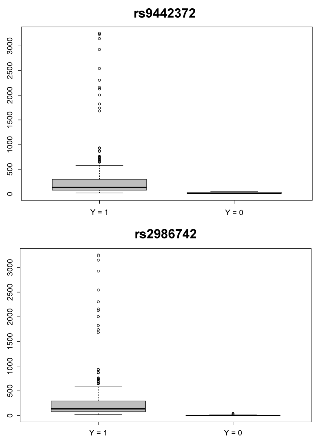
Figure 1.
Box plots of anti-cyclic citrullinated peptide (CCP) values of the case () and control () groups for the two top-ranked single nucleotide polymorphisms: “rs9442372” (upper panel) and “rs2986742” (lower panel).
In Table 3, we provide the highest posterior credible sets for and , which represent the effect of the secondary phenotype on the disease status and the genetic effect on the secondary phenotype, respectively. In Bayesian inference, “credible set” terms are generally used instead of “confidence interval”. Actually, a credible set can be obtained by posterior distribution. The highest posterior density interval is defined by minimizing the length of interval satisfying .
Table 3.
Highest posterior density credible sets for the parameters of interest ().
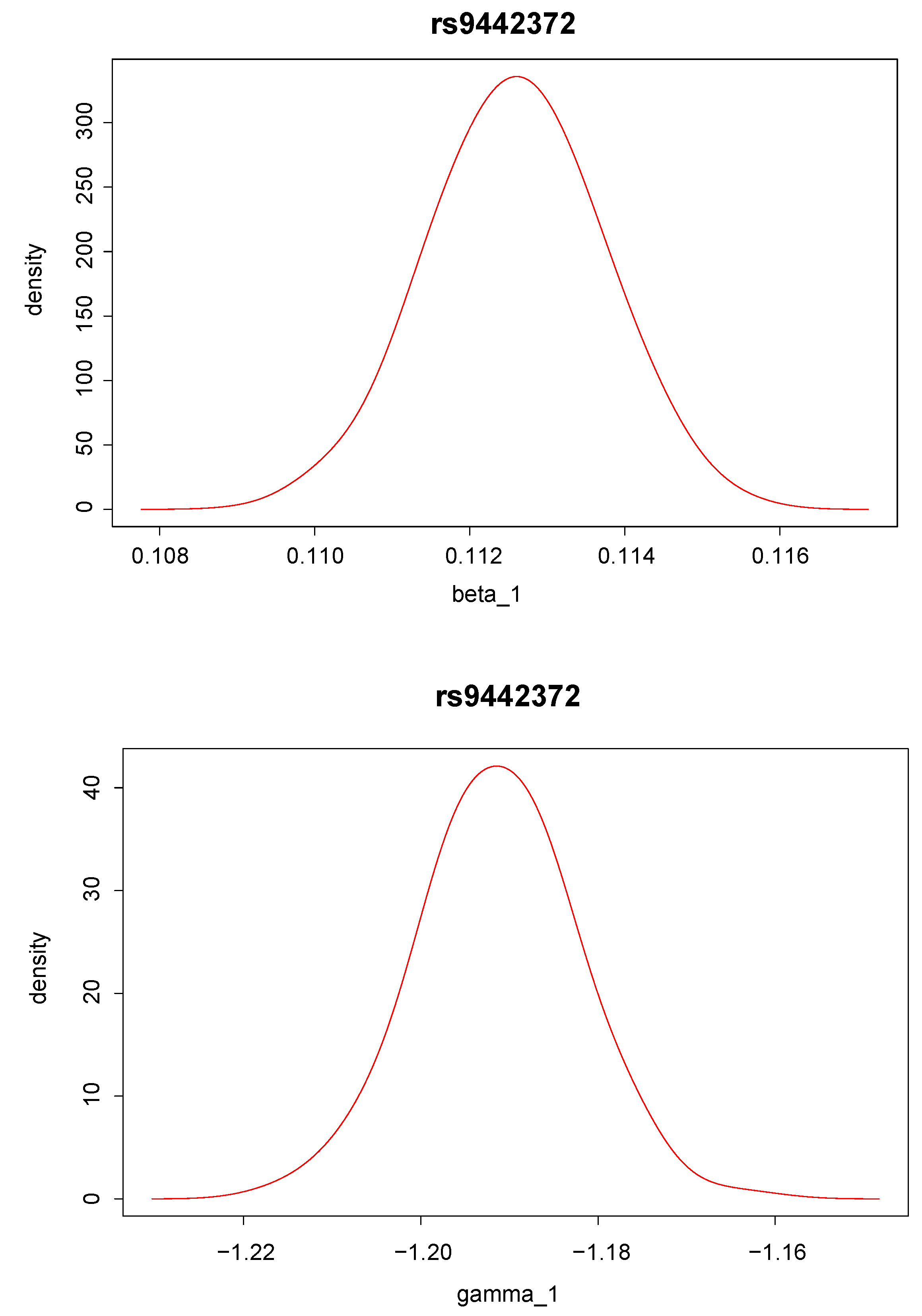
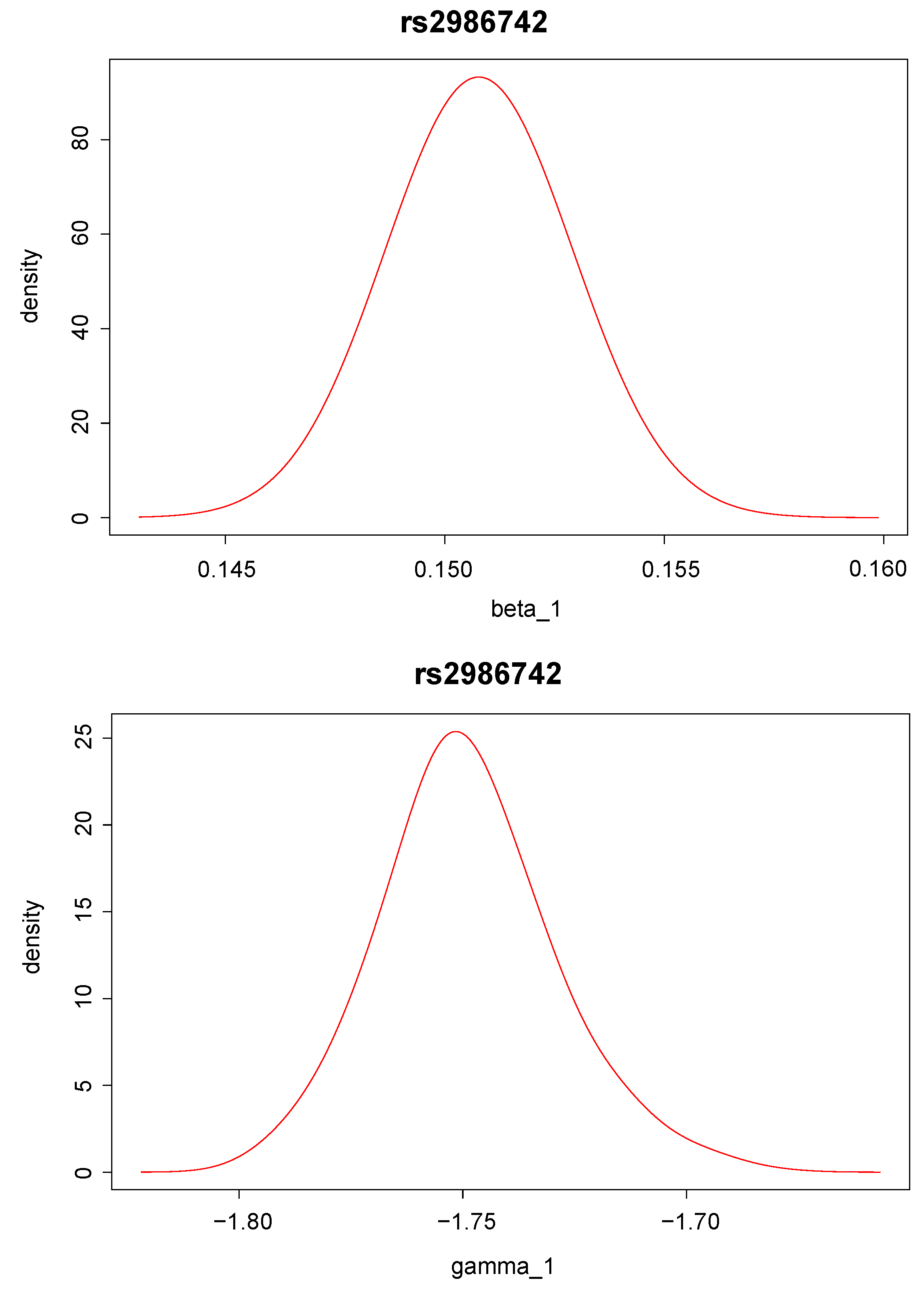
Posterior density distributions of and for the top two ranked SNPs, “rs9442372” and “rs2986742”, are plotted in Figure 2 and Figure 3. For example, for the top ranked SNP “rs9442372”, the posterior means for and are 0.113 and −1.193, respectively. The positive posterior mean for implies that knowing the anti-CCP values seems to increase the chance of RA. The magnitude of the posterior mean for implies that the SNP exerts quite a large genetic effect on the anti-CCP value.
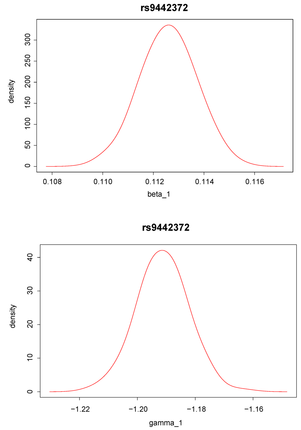
Figure 2.
Posterior distribution of (upper panel) and (lower panel) for single nucleotide polymorphism “rs9442372”, which has the largest Bayes factor.

Figure 3.
Posterior distribution of (upper panel) and (lower panel) for single nucleotide polymorphism “rs2986742”, which has the second largest Bayes factor.
7. Discussion
When information on the secondary phenotype is available only for the case group due to cost and different data sources in genome-wide association studies, it is not feasible to fit a linear regression incorporating stratum-specific missing data. On the other hand, fitting a linear regression model ignoring supplementary phenotype data may provide limited knowledge regarding genetic association. In this paper, we have considered Bayesian genetic association testing when only partial secondary continuous phenotype trait values are available and investigated the genetic effects on disease status through the intermediate secondary phenotype. We illustrate the use of Bayes factors in GWAS for selected SNPs whose p-values from logistic regression are highly significant. Using a Bayesian approach for inference, available but incomplete information is reflected in the model through the prior established on the parameter. For example, we set a strong prior on to make use of the knowledge that the partially-observed anti-CCP values are lower for the control group than the case group. In addition, we were able to incorporate the partially-observed secondary outcomes related to the disease in the model and generated the missing outcomes in the control group.
Our setup is that secondary phenotypes are completely missing in the control group due to different sources of data. In such a case, we cannot apply regression analysis, and we proposed the Bayesian approach as a reasonable option to model the data. We present the analysis of the RA data primarily as an example illustrating the potential of the Bayesian approach based on joint likelihood when secondary phenotypes are completely missing in the control group, except the knowledge that secondary phenotype values are lower for the control group than in the case group. Our approach can be applicable to the whole genome-wide association study. The running time per SNP was about 480 s per 20,000 iterations using R Version 3.1.3 on a personal computer (Intel Core I-7 at 3.40 GHZ).
With the liability threshold model, Falconer [25] supposed that there is a hypothetical and continuous attribute, which he referred to as the individual’s “liability” to the disease of interest, and all individuals above a certain threshold are affected with the disease. This notion of liability is similar to a latent variable in statistics, and his assumption is limited to normally distributed liability with equal variance for the case and the control groups. However, our motivation was to model “mediated pleiotropy”, where a causal gene affects one phenotype (anti-CCP) that lies on the causal path to another phenotype (RA status), and thus, an association occurs between the observed gene and both phenotypes. There are multivariate analyses jointly analyzing more than one phenotype in a unified framework and test for the association of multiple phenotypes with a genetic variant, for example multivariate analysis of variance (MANOVA). However, MANOVA or other ordinary regression approaches cannot handle the case when the first phenotype is not available for the whole control group. Our approach handles such a case, and the Bayesian framework allows us to test the association between a genetic variant and the phenotype of interest making use of partial information on the missing phenotypes in the control group. We present the results based on real data analysis to illustrate the potential of the Bayesian approach proposed in this paper. The signal presented in our table should be interpreted with caution, and it would be nice to validate it using independent data sample.
In genome-wide association studies, there is a variety of efforts to recruit more study subjects, because we need to test for a huge number of genetic variants with a rather small number of subjects compared to the number of SNPs. This may include collecting data at both population and family levels and combining data from different resources. Ascertainment bias happens when there is more intensive screening for the outcome among the affected than among the unaffected. Then, the case-control ratio in the available sample does not necessarily represent the prevalence of the disease at the population level due to the way the data are collected. There are several attempts to explore or explicitly incorporate ascertainment bias, for example conducting sensitivity analysis or conditional likelihood approach (Lachance and Tishkoff [26] and Haghighi and Hodge [27]). We leave the issue of incorporating ascertainment bias in Bayesian framework as future work.
The use of a fully-Bayesian approach for hypothesis testing eliminates the difficulties of constructing estimators, because no estimation is required; instead, hypothesis tests are obtained directly from the likelihood, with nuisance parameters integrated out. If parameter estimates are required, they can be obtained from the posterior distribution as posterior means and credible intervals, as demonstrated in this article.
The Bayes factor is a summary measure that provides an alternative to the p-value for the ranking of associations or the flagging of associations as significant. Andrews [28] showed the relationship between the Bayes factors and Wald, likelihood ratio and score statistics under quite general priors. Instead of reporting p-values, whose interpretation depends on the sample size, we recommend reporting Bayes factors with p-values. For a given test statistic, p-values only measure significance, whereas Bayes factors integrate both the significance and the sample size to detect an association. One benefit of reporting Bayes factors is that they are more appropriate measures than p-values when comparing results across GWAS with different sample sizes, which is a frequent situation in GWAS for common diseases.
The case subjects that we made available for our analysis comprise independent individuals who have met the American College of Rheumatology criteria for rheumatoid arthritis. These cases comprise a single member of 445 sib-pairs that were studied as a part of the North American Rheumatoid Arthritic Consortium and an additional 423 cases who were not selected for family history. The cases were recruited from across the United States. Cases are predominantly of Northern European origin. The control subjects, derived from the New York Cancer Projects, were enrolled in the New York metropolitan area. These controls are enriched for individuals of Southern European or Ashkenazi Jewish ancestry compared to cases [12]. The problem of non-random ascertainment has been usually dealt with by formulating a conditional likelihood, which leads to the removal of some individuals from the study in order to avoid an outcome-dependent ascertainment bias. With our data, we did not think that our results are affected by case-control ascertainment, because the unrelated control group was obtained quite independently from the case subjects. Population stratification due to different ancestries within Europe might exist in our case-control data, and incorporating such stratification in the analysis is beyond the scope of this paper.
Acknowledgments
This research was supported by the year 2015 Yeungnam University Research Grant. This work is based on the GAW16 data gathered with the support of grants from the National Institutes of Health (NO1-AR-2-2263 and RO1-AR-44422, Peter K. Gregersen, PI) and the National Arthritis Foundation.
Author Contributions
Minjung Kwak conceived and designed the research; Yongku Kim and Minjung Kwak analyzed the data and interpreted the results; Yongku Kim and Minjung Kwak wrote and revised the manuscript. Both authors have read and approved the final manuscript.
Conflicts of Interest
The authors declare no conflict of interest.
References
- Draper, N.R.; Smith, H. Applied Regression Analysis, 3rd ed.; Wiley: New York, NY, USA, 1998. [Google Scholar]
- Chatterjee, N.; Carroll, R.J. Semiparametric maximum likelihood estimation exploiting gene-environment independence in case-control studies. Biometrika 2005, 92, 399–418. [Google Scholar] [CrossRef]
- Agresti, A. Categorical Data Analysis; Wiley: New York, NY, USA, 1990. [Google Scholar]
- Zheng, G.; Freidlin, B.; Gastwirth, J.L. Robust genomic control for association studies. Am. J. Hum. Genet. 2006, 78, 350–356. [Google Scholar] [CrossRef] [PubMed]
- Chatterjee, N.; Kalaylioglu, Z.; Moslehi, R.; Peters, U.; Wacholder, S. Powerful multilocus tests of genetic association in the presence of gene-gene and gene-environment interactions. Am. J. Hum. Genet. 2006, 79, 1002–1016. [Google Scholar] [CrossRef] [PubMed]
- Maity, A.; Carroll, R.J.; Mammen, E.; Chatterjee, N. Testing in semiparametric models and interaction, with applications to gene-environment interactions. J. R. Statist. Soc. B 2009, 71, 75–96. [Google Scholar] [CrossRef] [PubMed]
- The Welcome Trust Case Control Consortium (WTCCC). Genome-wide association study of 14,000 cases of seven common diseases and 3000 shared controls. Nature 2007, 447, 661–678. [Google Scholar]
- Wu, C.; Zheng, G.; Kwak, M. A joint regression analysis for genetic association studies with outcome stratified samples. Biometrics 2013, 69, 417–426. [Google Scholar] [CrossRef] [PubMed]
- He, J.; Li, H.; Edmondson, A.C.; Rader, D.J.; Li, M. A Gaussian copula approach for the analysis of secondary phenotypes in case-control genetic association studies. Biostatistics 2012, 13, 497–508. [Google Scholar] [CrossRef] [PubMed]
- Stephens, M.; Balding, D.J. Bayesian statistical methods for genetic association studies. Nat. Rev. Genet. 2009, 10, 681–690. [Google Scholar] [CrossRef] [PubMed]
- Xu, J.; Yuan, A.; Zheng, G. Bayes factor based on the trend test incorporating Hardy-Weinberg disequilibrium: More powerful to detext genetic association. Ann. Hum. Genet. 2012, 76, 301–311. [Google Scholar] [CrossRef] [PubMed]
- Amos, C.I.; Chen, W.V.; Seldin, M.F.; Remmers, E.F.; Taylor, K.E.; Criswell, L.A.; Lee, A.T.; Plenge, R.M.; Kastner, D.L.; Gregersen, P.K. Data for genetic analysis workshop 16 Problem 1, association analysis of rheumatoid arthritis data. BMC Proc. 2009, 3. [Google Scholar] [CrossRef]
- Worthington, J.; Barton, A.; John, S.L. The Epidemiology of Rheumatoid Arthritis and the Use of Linkage and Association Studies to Identify Disease Genes; Springer-Birkhäuser: Basel, Switzerland, 2005. [Google Scholar]
- Huizinga, T.W.; Amos, C.I.; van der Helm-van Mil, A.H.; Chen, W.; van Gaalen, F.A.; Jawaheer, D.; Schreuder, G.M.; Wener, M.; Breedveld, F.C.; Ahmad, N.; et al. Refining the complex rheumatoid arthritis phenotype based on specificity of the HLA-DRB1 shared epitope for antibodies to citrullinated proteins. Arthritis Rheum. 2005, 52, 3433–3438. [Google Scholar] [CrossRef] [PubMed]
- Kroot, E.J.; de Jong, B.A.; van Leeuwen, M.A.; Swinkels, H.; van den Hoogen, F.H.; van’t Hof, M.; van de Putte, L.B.; van Rijswijk, M.H.; van Venrooij, W.J.; van Riel, P.L. The prognostic value of anti-cyclic citrullinated peptide antibody in patients with recent-onset rheumatoid arthritis. Arthritis Rheum. 2000, 43, 1831–1835. [Google Scholar] [CrossRef]
- Chen, L.; Zhong, M.; Chen, W.V.; Amos, C.I.; Fan, R. A genome-wide association scan for rheumatoid arthritis data by Hotelling’s T2 tests. BMC Proc. 2009, 3. [Google Scholar] [CrossRef]
- Suzuki, A.; Yamada, R.; Chang, X.; Tokuhiro, S.; Sawada, T.; Suzuki, M.; Nagasaki, M.; Nakayama-Hamada, M.; Kawaida, R.; Ono, M.; et al. Functional haplotypes of PADI4, encoding citrullinating enzyme peptidylarginine deiminase 4, are associated with rheumatoid arthritis. Nat. Genet. 2003, 34, 395–402. [Google Scholar] [CrossRef] [PubMed]
- Begovich, A.B.; Carlton, V.E.; Honigberg, L.A.; Schrodi, S.J.; Chokkalingam, A.P.; Alexander, H.C.; Ardlie, K.G.; Huang, Q.; Smith, A.M.; Spoerke, J.M.; et al. A missense single-nucleotide polymorphism in a gene encoding a protein tyrosine phosphatase (PTPN22) is associated with rheumatoid arthritis. Am. J. Hum. Genet. 2004, 75, 330–337. [Google Scholar] [CrossRef] [PubMed]
- Sasieni, P.D. From genotypes to genes: Doubling the sample size. Biometrics 1997, 53, 1253–1261. [Google Scholar] [CrossRef] [PubMed]
- Berger, J.O.; Sellke, T. Testing a point null hypothesis: The irreconcilability of p values and evidence. J. Am. Stat. Assoc. 1987, 82, 112–122. [Google Scholar] [CrossRef]
- Kass, R.E.; Raftery, A.E. Bayes factors. J. Am. Stat. Assoc. 1995, 90, 773–795. [Google Scholar] [CrossRef]
- Casella, G.; Berger, R.L. Reconciling Bayesian and frequentist evidence in the one-sided testing problem (with discussion). J. Am. Stat. Assoc. 1987, 82, 106–111. [Google Scholar] [CrossRef]
- Clogg, C.C.; Goodman, L.A. Latent structure analysis of a set of multidimensional contingency tables. J. Am. Stat. Assoc. 1984, 79, 762–771. [Google Scholar] [CrossRef]
- Coenen, D.; Verschueren, P.; Westhovens, R.; Bossuyt, X. Technical and diagnostic performance of 6 assays for the measurement of citrullinated protein/peptide antibodies in the diagnosis of rheumatoid arthritis. Clin. Chem. 2007, 53, 498–504. [Google Scholar] [CrossRef] [PubMed]
- Falconer, D.S. The inheritance of liability to certain diseases, estimated from the incidence among relatives. Ann. Hum. Genet. 1965, 29, 51–76. [Google Scholar] [CrossRef]
- Lachance, J.; Tishkoff, S.A. SNP ascertainment bias in population genetic analyses: Why it is important, and how to correct it. Bioessays 2013, 35, 780–786. [Google Scholar] [CrossRef] [PubMed]
- Haghighi, F.; Hodge, S.E. Likelihood formulation of parent-of-origin effects on segregation analysis, including ascertainment. Am. J. Hum. Genet. 2002, 70, 142–156. [Google Scholar] [CrossRef] [PubMed]
- Andrews, D.W.K. The large sample correspondence between classical hypothesis tests and Bayesian posterior odds tests. Econometrica 1994, 62, 1207–1232. [Google Scholar] [CrossRef]

© 2016 by the authors; licensee MDPI, Basel, Switzerland. This article is an open access article distributed under the terms and conditions of the Creative Commons by Attribution (CC-BY) license (http://creativecommons.org/licenses/by/4.0/).